AN ALGORITHM FOR THE SOLUTION OF A CLASS OF NONLINEAR LEARNING CURVE MODELS
USING GEOMETRIC PROGRAMMING
ARTHUR LAKES LIBRARY COLORADO SCHOOL of MINES
GOLDEN, COLORADO 80401
by
All rights reserved INFORMATION TO ALL USERS
The qu ality of this repro d u ctio n is d e p e n d e n t upon the q u ality of the copy subm itted. In the unlikely e v e n t that the a u th o r did not send a c o m p le te m anuscript and there are missing pages, these will be note d . Also, if m aterial had to be rem oved,
a n o te will in d ica te the deletion.
uest
ProQuest 10783571Published by ProQuest LLC(2018). C op yrig ht of the Dissertation is held by the Author. All rights reserved.
This work is protected against unauthorized copying under Title 17, United States C o d e M icroform Edition © ProQuest LLC.
ProQuest LLC.
789 East Eisenhower Parkway P.O. Box 1346
A thesis submitted to the Faculty and the Board of Trustees of the Colorado School of Mines in partial
fulfillment of the requirements for the degree of Master of Science (Mineral Economics).
Golden, Colorado 1990 Signed:
IrQ
Michael F. Pfennli Michael F. Pfen^il^g / Approved:ifr. R.E.D. wa«
Thesis Advisor
Golden, Colorado
k , 1990
M J o h n E.Tilton D m John E. Tilton Professor and Head,
Mineral Economics Department ii
ABSTRACT
Decision makers and accountants in the mining, petroleum, and manufacturing industries face ever
increasing problems in the allocation of competing resources such as labor and machinery hours in their
production sequences. In these industries where there are tasks subject to improvement as the result of learning by the workers, a commonly held hypothesis is that they learn in keeping with a predictable pattern. These learning
effects were first observed and documented in 1925 in the aircraft production industry. Since that time,
incorporation of learning effects into production sequence models has continued to occur primarily in the formulation phase. The underlying reason for this is that the
incorporation of learning effects in these models has caused mathematical problems in the solution attempts of previous work in this field. As a result, the collection of data to utilize these types of models has been at a
standstill in many industries.
In this thesis an optimizing algorithm is developed for solving a class of nonlinear resource allocation models in which learning effects are included. This algorithm is capable of solving multi-variable, constrained equations
with multiple degrees of geometric programming difficulty. The algorithm uses condensation and geometric
programming techniques applied to the model's objective function. The generated solutions are iteratively checked against the remaining constraints, until the optimal
solution is determined.
TABLE OF CONTENTS
Page A B S T R A C T ... iii LIST OF F I G U R E S ... vii ACKNOWLEDGEMENTS ... viii Chapter 1. INTRODUCTION TO NONLINEAR RESOURCE
ALLOCATION MODELS ... 1 1.1. Historical Summary of Learning
Curve T h e o r y ... 1 1.2. Review of the Standard M o d e l ... 7 1.3 Formulation of the Learning Model . . . 8
Chapter 2. A REVIEW OF PREVIOUS W O R K ... 15 2.1. The Lagrange Multiplier Approach . . . 16 2.2. The Reeves-Sweigert Approach ... 18 2.3. The Nonlinear Learning Effects (NOLLE)
A p p r o a c h ... 22 Chapter 3. DEFINITION OF THE LCMGP ALGORITHM . . . 26 3.1. Introduction to Geometric Programming . 2 6
3.2. Phase 1: Reformulation of the Problem . 28 3.3. Phase 2: The Problem S o l u t i o n ... 30 3.3.1. The Two-Variable Product-Mix Problem . 32 3.3.2. The Three-Variable Product-Mix Problem 41 Chapter 4. APPLICATION OF THE LCMGP ALGORITHM
TO A SET OF TEST P R O B L E M S ... 50 v
Chapter 5. RESULTS AND SUGGESTIONS FOR
FURTHER R E S E A R C H ... 62 5.1. Discussion of the R e s u l t s ... 62 5.2. Suggestions for Further Research . . . 63 REFERENCES CITED ... 65
LIST OF FIGURES
Page Figure 1.1. The 80% Learning Curve Plotted with
Arithmetic Scales on Both A x e s ... 3 Figure 1.2. The 80% Learning Curve Plotted with
a Double Logarithmic Scale ... 3 Figure 1.3. Various Learning Curve Models With
the Same Value of Direct Labor Hours
Per Unit at 100 U n i t s ... 4 Figure 1.4. Typical Learning Curves Requiring One
Direct Labor Hour to Manufacture the
First Unit (i.e., K = 1 ) ... 6
Figure 3. Flowchart for the LCMGP Algorithm... 31
ACKNOWLEDGEMENTS
This thesis is dedicated to Dr. R.E.D. Woolsey, a devoted teacher, consummate scholar, and creative force in the field of operations research. He has taught me to
"stand at the edge and not be afraid to stretch the first rope to the other side." I will be eternally in his debt. I would like to take this opportunity to express my thanks to the U. S. Army for providing me the opportunity to pursue a master of science degree at Colorado School of Mines.
I would also like to acknowledge the help of Joseph H. Katz, Adam Hoyt, and CPT Robert Clayton in the computer coding of the algorithm in this thesis.
Additionally, I would like to acknowledge the help of CPT David A. Kickbusch in the printing of the graphs in this thesis.
Finally, I would like to acknowledge the patience and perseverence of my wife Anne, whose support has been
unwavering throughout my program of study at CSM.
Chapter 1
INTRODUCTION TO NONLINEAR RESOURCE ALLOCATION MODELS
1.1. Historical Summary of Learning Curve Theory
Learning effects were first observed and documented in the aircraft production industry in 1925 by Wright
(1936, 122-124). As the shortage of skilled manpower developed at the outbreak of the Second World War, the
Department of Defense (DOD) became interested in methods to reduce the costs of aircraft and ship production. DOD
commissioned the Stanford Research Institute to study the effects of labor inputs versus commodity outputs of several aircraft firms during the war. This database of direct
labor hours and aircraft output in the production sequences of several aircraft firms was later statistically analyzed to determine whether there was a relationship.
As summarized by Andress (1954, 87), the basic theory of the learning effect is simple: workers learn as they work; the more often they repeat an operation, the more efficient they become, with the result that the direct labor output per unit declines. Ebert (1976, 171)
identified several sources of productivity changes. These productivity changes may take the form of (but are not
limited to) :
1. Facility layout modifications 2. Product engineering modifications 3. Equipment redesign
4. Changes in employee skills
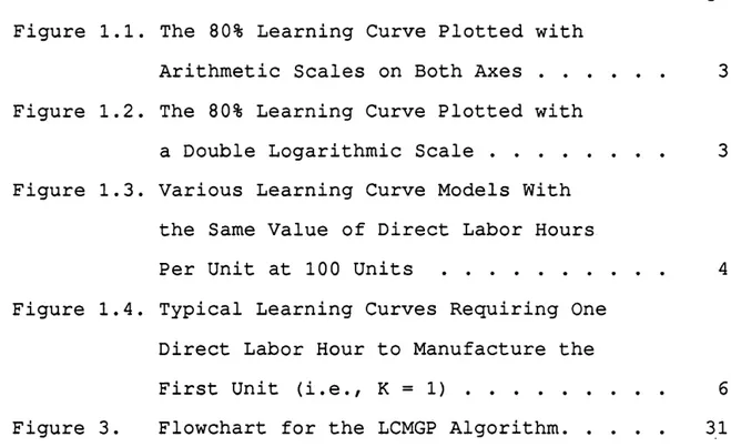
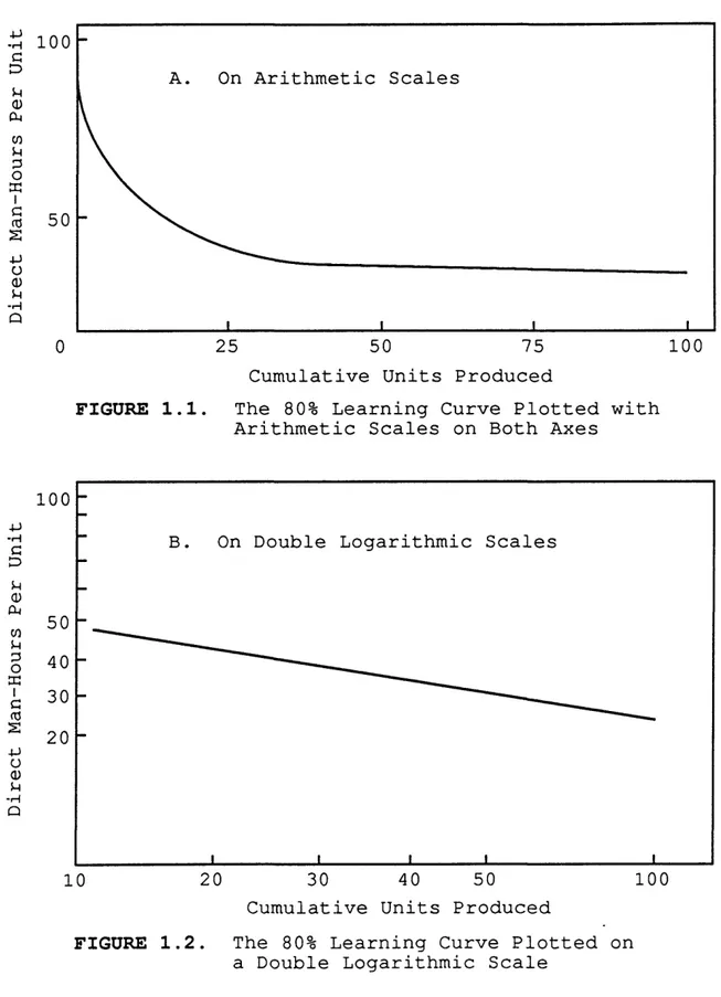
The predictable pattern by which this learning
occurred became known as the learning curve. Other authors have referred to the learning curve as the progress curve, the improvement curve, and the experience curve. An example of an 80% learning curve on arithmetic scales (see figure
1.1) and double logarithmic scales (see figure 1.2)
demonstrates the observed relationship between direct labor hours per unit and cumulative units produced. When graphed on double log paper, the learning curve should be a
straight line.
In other words, an 80% learning curve (or .80 learning rate) means that a 2 0% reduction in costs is expected to occur as the cumulative number of units produced doubles.
Learning curves provide a means of calibrating the decline in marginal labor hours as workers become more
familiar with a particular task or as greater efficiency is introduced into the production process.
D i r e c t M a n -H o u r s P e r U n i t D i r e c t M a n -H o u r s P e r U n i t 100 A. On Arithmetic Scales 100 25 50 75 0
Cumulative Units Produced
FIGURE 1.1. The 80% Learning Curve Plotted with Arithmetic Scales on Both Axes
100
On Double Logarithmic Scales
20
50 100
20 30 40
10
Cumulative Units Produced
FIGURE 1.2. The 80% Learning Curve Plotted on a Double Logarithmic Scale
D i r e c t L a b o r H o u r s P e r U n i t
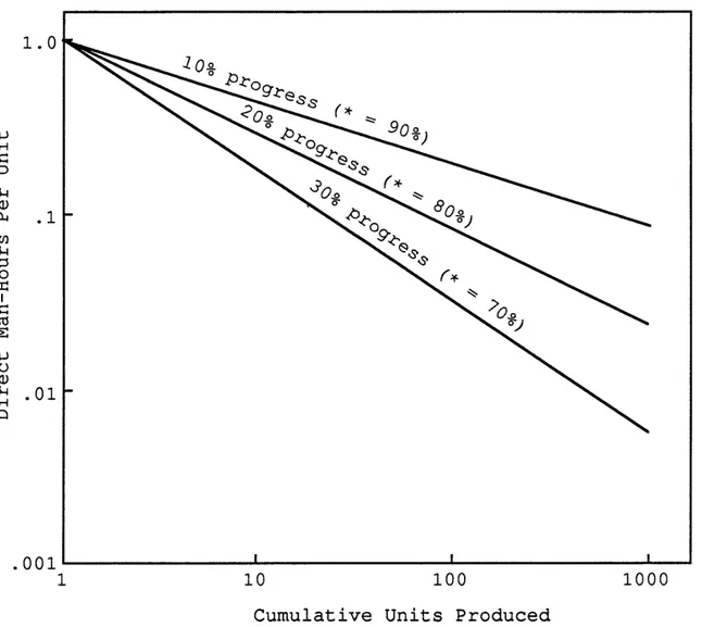
Many geometric versions of the learning curve have been developed (Yelle 1979, 304) from the initial data obtained from the Stanford Research Institute, as well as follow-on studies. They are shown in figure 1.3 and
include:
1. The log-linear model 2. The plateau model 3. The Stanford-B model 4. The Dejong model 5. The S-model Plateau Model 1000 S-Model Log-linear Model 100 DeJong Model Stanford-B Model 1000 10 100 1
Cumulative Units Produced
FIGURE 1.3. Various Learning Curve Models with the Same Value of Direct Labor Hours Per Unit at 100 Units
The reason for the differing models stems from the fact that the log-linear model does not always provide the best fit in all situations. However, the log-linear model has been, and still is, by far the most widely used model in manufacturing and production models, as noted by
Balkaoui (1986, 24). Accordingly, this study will focus on the analysis of the log-linear model of learning curve theory.
Learning curves follow the mathematical function:
Y = KXn (1.1)
where
Y = The number of direct labor hours required to produce the Xth unit
K = The number of direct labor hours required to produce the first unit
X = The cumulative quantity of output to be produced n = log */log 2 = The learning index
* = The learning rate (the amount of productivity improvement expected as the number of units produced doubles). For example, an 80% learning
curve (or .80 learning rate) means that a 2 0% reduction in costs is expected to occur as the cumulative number of units produced doubles. These learning rates are normally determined from industrial data from the start of the production sequence in question or other similiar
production sequences.
Some typical learning curves with different learning rates are shown in figure 1.4 (Yelle 1979, 303). The
D i r e c t M a n -H o u r s P e r U n i t .001 100 1000 10 1
Cumulative Units Produced
FIGURE 1.4. Typical Learning Curves Requiring One Direct Labor Hour to Manufacture the First Unit (i.e K = 1)
steeper the slope, the greater the learning effect. Thus, the 30% progress curve in figure 1.4 represents a greater learning effect (owing to higher labor content) than the
1 0% progress curve.
1.2. Review of the Standard Model
The general product-mix problem as discussed in Johnson and Winn (1979, 202-204) and Leinert (1982, 1-4), is one of several well-known planning problems which incorporate learning effects in their formulation. This problem (hereafter Standard Model) is of the form:
Maximize n (1 .2 ) j=l subject to n (1.3) j=l and Xj >= 0, j = 1, 2, ... (1.4) where Xj = level of activity j (j = 1, 2, . .
Fj = unit "profit" from activity j- Z = total "profit" from all activities
Aj__i = amount of resources i consumed by each unit of activity j
= amount of resource i available (i = I, 2, . . ., m)
1.3. Formulation of the Learning Model
The original formulation of the Standard Model
assumes that scarce resources will be allocated in such a manner as to maximize the value of the objective function. Additionally, as stated in Liao (1979, 118),
One of the implicit assumptions in the model is the expectation of constant operational
efficiency. In other words, all technological coefficients, A^j, are constant.
When learning effects are present in a portion of the production sequence upon which this model is based, the assumption of constant operational efficiency is violated. The resources whose consumption is affected by learning effects can be thought of in economic terms as the variable costs of the production sequence. In other words, for a fixed labor force, production capacity expands and marginal costs decrease automatically as learning takes place.
In economic terms, the general form of the learning curve model can be thought of as a problem to maximize the profits (Revenue - Costs[both fixed and variable]) of a production sequence subject to the limited amounts of
resources are utilized in processes in which learning effects are present.
If learning effects are present in the production sequence, then we must incorporate two changes into the Standard Model, as discussed in Reeves and Sweigert (1981, 205-206), to arrive at a more realistic model.
Change 1. As learning occurs, the amount of resource A^j required to produce each unit of the jth activity
decreases. Therefore, the technological coefficients Aj_j in the Standard Model can be formulated mathematically as
A i;j* = A i;j XjBi3 (1.5) where
Aji* = the marginal rate of substitution of resource i for product j reflecting learning
Aj_j and Xj are as previously defined
= the learning index of resource i in the production of product j
Note that B^j = log *ij/log 2, where *ij is the learning rate (the amount of productivity
improvement expected as the number of units produced doubles).
As noted by Smunt (1986, 479), *ij from industries will normally be in the range .70 < *ij < 1, and therefore,
Bj_j values will be in the range -.5 < Bj_j < 0.
Change 2. When learning effects are present, Fj, the marginal contribution to the objective function (equation
[1.2]) for product j would be an increasing rather than a constant function of the level of production of product j. Thus, in the objective function, Fj must be replaced by
Pj = the unit selling price of product j
VOj = the total unit variable cost not subject to learning required for each unit of product j
V^ = the unit variable cost of resource i which is subject to learning effects
Aj_j* = as defined by equation (1.5)
Reformulating the Standard Model (equations [1.2] through [1.4]) using the changes specified in equations
(1.5) and (1.6) and assuming that only the first g
resources are subject to learning effects, we can now write the general Learning Model as follows:
Maximize m (1.6) where j-1 n j=l i=l
subject to n A i j Xj^ <— i - 1/ 2/ . . . , g (1.8) i=l n ^ A ij Xj <= bi, i = g+1, g+2, . .., m j=l and Xj >= 0, j = l , 2,..., n (1.10) (1.9)
It is a generally accepted modeling principle that as models are further developed to become more realistic, they tend to become more difficult to solve. In this case, the Learning Model is a nonlinear programming problem in which the objective function is convex and the learning functions in the constraints are concave. As stated by Reeves and Sweigert (1981, 206):
Incorporating the effects of learning into the constraints increases the size of the feasible region outward from the origin allowing more units of products to be produced with the same level of resources. Unfortunately such a loosening of
constraints involving learning makes the feasible region nonconvex. Thus, [Learning Model] involves the maximization of a convex function over a
nonconvex set. Unlike the [Standard Model], there is no guarantee in general that a local optimum solution to [Learning Model] is global, and there can be many local optima.
An example of a Learning Model or product-mix problem as given in Liao (1979, 121) is shown below. (This problem will be further analyzed in chapter 3).
A plant is considering beginning the production of three new products (X^, X2, and X3). The plant manager must determine how to allocate resources to accomplish
production goals of the products for the first month. The plant has 14,400 units of material, 5,920 machine hours, and 13,026 direct labor hours available in the first month.
According to the plant engineer's studies, material requirements for production of one unit of products X-j_, X2, and X3 are 10, 12, and 15 units. Additionally, plant
accounting records indicate that in a similiar process, direct labor hour and machine hour learning effects have been observed. (Another method of obtaining this data would be to run pilot runs of the new operation.) Using this
data, the plant accountants have developed expected learning rates and the number of direct labor hours and machine hours to produce the first unit of products X X 2, and X3. They are shown below.
Product A Product B Product C
Expected Learning Rate 80% 85% 90%
Direct labor hrs required
to produce the first unit 40 32 36
Machine hrs required to
produce the first unit 24 20 14
are $381, $320, and $377. The plant expects no demand constraint for the product at its current capacity
production. The unit variable costs not subject to learning are $28, $25, and $30 for products X-j_, X2, and X3.
Using equations (1.7) through (1.10), this product- mix problem can be formulated as a nonlinear programming problem as follows: Maximize Z(X1,X2,X3) = (353XX - 320X1 *67807) + (295X2 - 256X2 *76553) + (347X3 - 2 8 8X3•8480°) subject to M(X1,X2,X3) = 10X1 + 15X2 + 1 2X3 <= 14400 N(X1,X2,X3) = 24X1 *67807 + 20X2 *76553 + 14X3 *84800 <= 5920 0(X1,X2,X3) = 40X1 ‘67807 + 32X2 *76553 + 3 6X3 • 8 4 8 0 0 <= 13026
where M, N, and 0 represent restriction functions of the material, direct labor, and machine hours available in the
first month.
As noted by Chen (1983, 170), the optimal solution of these types of Learning Models has proved difficult, if not
impossible. Previous attempts at the solution of the production sequence models with learning effects have universally used the Standard Model and the Learning Model as a common reference point in their analysis. Chapter 2 is a review of three of these previous solution methods.
Chapter 2
A REVIEW OF PREVIOUS WORK
In this chapter three different methods of solving the Learning Model (equations [1.7] through [1-10]) will be discussed using the specific numerical problem as given in Liao (1979, 121) and intoduced in chapter 1. The problem is to find X - j X2/ X3, where X-^, X2, and X3 >= 0, such that
Maximize subject to M(XX, X2, X3) = 10XX + 15X2 + 1 2X3 <= 14,400 (2.2) Z(x1# X 2 , x 3 ) = (353XX - 320X1 67807 + (295X2 - 256X2 ,7655S + ( 3 4 7 X 3 - 2 8 8 X 3 84800) (2 .1 ) N(XX, X2/ X 3) = 24XX 6 7 8 0 7 + 20X2 *7 6 5 5 3 + 14X3 84800 <= 5, 920 (2.3) 0(X1, X2/ X 3) = 40XX 6 7 8 0 7 + 32X2 * 7 6 5 5 3 + 3 6 X 3 •84800 <= 13, 026 (2.4)
2.1. The Lagrange Multiplier Approach
The first approach to solving the problem represented by equations (2.1) through (2.4) is the application of the method of Lagrange multipliers as proposed by Liao (1979,
121) and discussed by Leinert (1982, 16). (In my
explanation of this method, lm-j_, ln^, and lm^ represent the three Lagrange multipliers.) This method is perhaps the most well-known to economists where equations (2-1) through
(2-4) are replaced by a new function F(X^/ x3' ^m i' lm2, 1^3) given by
F (X^, X21 X3, lm-j_, lm2, I1TI3) = Z (X^, X2, ^3^
+ lm1M(X1, X2,X3) + lm2N(X1, X2/ X3) + lm30(X1, X2/ X3)
where lm^, lm2, and lm3 are the Lagrange multipliers. In order to optimize F, F must be partially differentiated with respect to each of the six variables, X X 3/ X3, lm-j_,
ln^, and lm3, resulting in six partial derivative
equations. Then the six equations are set equal to zero and solved simultaneously to obtain the solutions for X^, X2/ X3, lm-j_, 1^2' ^m 3' anc* z> These first order conditions
(where L represents the Lagrangian function, F[X^/ X2/ X3,
a£/axx » (216.98 - 16.2712 - 27.1213)Xx“ *32193 + 1 0 ^ = 353 a£/ax2 = (195.97 - 15.3112 - 24.5013)X2" *23447 + 151x = 295 a£/ax3 = (244.24 - 11.8712 - 30.5313)X3” *15200 + 121x = 347 ^£/aim1 = 10XX + 15X2 + 12X3 = 14400 a£/aim2 = 24X-L*67807 + 20X2 *76553 + 14X3 *84800 = 5920 a£/aim3 = 40X1 *67807 + 32X2 *76553 + 36X3 *84800 = 13026
Solving the first three constraints in terms of lm-^ and setting them equal to one another reduces the number of variables for which solutions are needed to only five.
However, the amount of algebraic manipulation required to extract solutions for these variables is non-trivial. Theoretically, Liao should then have tested the solutions he generated from these first order conditions in the second order conditions to insure a global optimum. In essence, Liao identified only the first order conditions
(necessary) and omitted the testing of the solutions in the second order conditions.
As described in Reeves (1980, 170), this approach
leads to a suboptimal solution in that it cannot guarantee a global nor even a local optimum without checking the second
order conditions. As summarized by Leinert (1982, 17): A correct application of the Lagrange multipliers would require an application of the Kuhn-Tucker conditions, which would necessitate the solution of N simultaneous equations in N unknowns. This problem has at this point in time [and still has] no reliable closed-form solution.
Essentially, Liao failed to realize that in the case of inequality-constrained mathmatical programming problems, Kuhn-Tucker theory is the proper extension of the Lagrange multiplier effect. As noted by Reeves (1980, 169), even the properly applied Kuhn-Tucker theory would have required the identification of all Kuhn-Tucker points (local optima) before determining a global optimum. In most realistic sized problems, the completion of these tasks is neither practical nor computationally feasible.
2.2. The Reeves-Sweigert Approach
The second approach to solving the Learning Model was proposed by Reeves and Sweigert in 1981. In this two stage approach, Reeves first converts equations (2.1) through
(2.4) to a series of increasingly tight linear
approximating models. The resulting linear programming
problem generates a superoptimal solution using the simplex algorithm. In the second stage of the approach, upper and lower bounds for each of the variables are substituted into
the linear programming problem in different combinations (using a branch and bound technique) until the solution achieves a feasible and globally optimal solution.
In the first stage of this approach, linear outer envelope approximations are constructed for each nonlinear term in the objective function and in the constraints
subject to learning effects (see equations [1.7] and [1.8]). More specifically, as summarized by Reeves and Sweigert (1981, 207), each nonlinear term of the form
is replaced by
^ . i + b i j _ L l j l+bij (X. - L l j ) + L 1;j1+bi3
U Xj - Lj_j (2.5)
where Lj_j is a lower bound for Xj (j = 1, 2, ..., n) and Uj_j is the maximum value of Xj determined from all of the constraints (both those subject to and those not subject to learning effects). As stated by Leinert (1982, 18),
equation (2.5) "is just a linear equation in Xj which agrees with each original nonlinear term at Lj_j and uij*"
In the problem outlined in equations (2.1) through (2.4), the first stage of the Reeves-Sweigert approach is demonstrated as follows. First, generate upper and lower bounds for each of the variables in the problem from the
constraints, assuming each of the other variables is equal to zero. The lower bound for each of the variables in this problem is zero. By setting two of the three variables in each of the constraints equal to zero and successively solving for the remaining variable, the upper bounds are generated for each of the variables as follows:
0 <= Xx <= 1440 0 <= X2 <= 960 0 <= X3 <= 1220
Second, using these upper bounds on each of the
variables, those terms subject to learning in the objective function and the constraints are replaced with an
approximated linear term. (353X^ - 320X-j_ * 67807) be replaced by {353 - [320 (1440) *67807/1440]
}X1
= 322.21XX in the objective function. Additionally, 24X-j_* 8 7 8 8 7 and40X<l* 8 7 8 8 7 in the constraint equations would be replaced
with 24 (1440) *67807/1440 = 2.31X1 and 40 (1440) •67807/1440 = 3.85X«]_. The resulting approximated linear programming
problem is as follows:
Maximize
subject to
M(Xlf
X2, X3) = 10XX + 15X2 + 1 2X3 <= 14,400 N(XX, X2, X3) = 2.3 1X3^ + 3.99X2 + 4.76X3 <= 5,920 0(XX, X2, X3) = 3.85XX + 6.39X2 + 12.25X3 <= 13,026 The resulting approximated linear programming problem is then solved using the simplex algorithm. As the results of this step in the approach produce superoptimal results, these results are the initial start point in the branch and bound technique of part two of the approach.The branch and bound technique is an iterative approach to the solution of the problem which uses
different combinations of the upper and lower bounds of each of the variables in the approximated linear
programming problem from the first stage. Substitution of all possible combinations continues until the objective function value is maximized at global optimality.
This part of the approach is not difficult in
problems with only a few variables, but as the size of the problem becomes more realistic, the time and cost
investments to approach optimality rapidly become computationally and practically infeasible. These
computational problems are the main shortcomings of the approach.
2.3. The Nonlinear Learning Effects (NOLLE) Approach
This two-stage approach was developed (Leinert 1982) at the Colorado School of Mines. The first stage of the approach is the transformation of the learning model into the standard geometric programming format where the
objective function is converted to a minimization and the constraints are converted to the <= 1 format of the right-
hand side. This procedure will be discussed in chapter 3 as it is the same preprocessing step in the new algorithm.
The second stage of the approach replaces the linear terms in the transformed problem in both the objective
function and constraints not subject to learning with nonlinear terms of the general form k X j ^ where k is a positive constant. This stage of the procedure essentially transforms the problem in standard geometric programming format into the Approximating Learning Curve Model (ALGM) and solves this problem using the simplex algorithm.
The transformation of the problem in standard geometric programming format into the ALCM uses the
following procedure (Leinert 1982, 26) for each Xj (j = 1,
2, . . ., n) :
Step 1: Find the upper bound on Xj from the linear constraints; call this value XjUBL.
Step 2: Find the upper bound on Xj from the nonlinear constraints; call this value XjUBNL.
Step 3: Find the least upper bound on Xj from both the linear and nonlinear constraints; call this value XjLUB.
Thus,
X jLUB = minimum (x jUBL' X jUBNL^
The terms in the objective function and in the linear constraints are then transformed using the XjLUB to obtain the ALCM. After the transformation, the ALCM is solved using the simplex algorithm.
Using the NOLLE algorithm, the product-mix problem of equations (2.1) through (2.4) is transformed into
Maximize Z = 3348.988X1 -67807 + 1219.962X2 •76553 + 709.539X3 -84800) (2.6) subject to M = 103.937x1 + 75X2 + 34.497X3 <= 14400 (2.7) N = 24X1 *67807 + 20X2 *7 6 5 5 3 + 1 4X3 *84800 <= 5920 (2.8)
0 = 40XX 67807 + 3 2x2 7 6 5 5 3 + 36X3 -84800
<= 13026 (2.9)
The coefficients of X-^ 67807 in equations (2.6) and (2.7) are determined as shown below.
From equation (2.2), the upper bound on X1 is 1440.
This value is determined by setting X3 and X3 equal to zero. Using the notation introduced in steps 1 through 3 above, X1UBL = 1440. From equations (2.3) and (2.4), the upper bounds on X^ are 3371.49 and 5078.55, and thus, X 1UBNL = 3371.49. Consequently, X 1LUB = 1440.
Additionally, the new coefficient of X^ in equation (2.6) is (353 (1440)1“ -67807 - 320) = 3348.988, and the new coefficient of X^ in equation (2.7) is 10 (1440) *6 7 8 6 7
= 103.9373. The coefficients of X2 and X3 in equations
(2.6) and (2.7) are obtained similiarly.
If a variable transformation of the form, Yj = Xj6^, is conducted of equations (2.6) through (2.9), the
resulting system of equations becomes a linear programming problem which is the solved through the use of the simplex algorithm. The NOLLE algorithm gives initially
feasible solutuions to the learning model which are either optimal or close to optimal. Additionally, it avoids the
difficulties of the Reeves-Sweigert approach which 1) initially gives infeasible solutions and 2) requires a branch-and-bound procedure. Finally, this approach does provide globally optimal solutions to learning models.
The last approach is superior to the first two approaches based on its global optimality and its computational ease.
Since only one of these three methods available for solving the learning model is adequate, another algorithm that neither depends on the branch-and-bound procedure nor requires the transformation to the ALCM is desirable. Such an algorithm will be developed in chapter 3.
Chapter 3
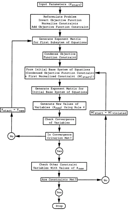
DEFINITION OF THE LCM6P ALGORITHM
The Learning Curve Model Geometric Programming (LCGMP) algorithm is a two phase process. The first of these phases is the reformulation of the original problem. The second phase is the application of some of the rules in Geometric Programming (G.P.). This thesis assumes the
reader has a basic understanding of G.P. The steps of the algorithm will be presented in a manner that assumes the reader is solving the problem by hand. However, a FORTRAN program implementing this algorithm is in an appendix to this thesis. A brief introduction to G.P. techniques is included prior to discussion of the algorithm.
3.1. Introduction to Geometric Programming
G.P. is a very useful tool in solving nonlinear equations of the type encountered in the learning curve model. However, as the number of terms in the problem becomes large relative to the number of variables,
conventional G.P. techniques must be augmented with the "Four Rules" as developed by Woolsey in 1969 (Woolsey and Swanson, 1975) and outlined by Woolsey (1988, 4).
where each variable is balanced within the system of equations (both a positive and negative power exist for each variable) and the degree of difficulty (DD) of the problem is zero. The DD of a problem is defined to be the total number of terms in the problem, minus the total
number of variables in the problem, minus one. Therefore, the specific product-mix problem discussed in chapter 2
[equations (2.1) through (2.4)] Maximize Z(X1,X2/X3) = (353X3^ - 320X1 -67807) + (295X2 - 256X2 *76553) + (347X3- 288X3 -84800) (3.1) subject to M(X1,X2,X3) = 10X1 + 15X2 + 12X3 <= 14,400 (3.2) N(X1,X2,X3) = 24X1 ’67807 + 20X2 ’7 6 5 5 3 + 14X3 -84800 <= 5,920 (3.3) 0(X1,X2,X3) = 40X1 ’67807 + 32X2 ,765S3 + 36X3 •84800 <= 13,026 (3.4)
Since the degree of difficulty of this problem is not zero, conventional G.P. techniques are not immediately
applicable.
3.2. Phase 1: Reformulation of the Problem
The general form of the Learning Curve Model
discussed in chapter 1 (equations [1.7] through [1.9]) can be reformulated as follows: Minimize n g j=l i=l subject to n (
^2
A ijx j1+Bij>/Bi <= 1, i = 1, 2, g (3.6) i=l n ( A ijx j) /^i <= !/ i = g + 1/ g + 2, ..., m (3.7) j=l and Xj >= 0, j = l , 2, ..., n (3.8)In this formulation, the original objective function, Z, is inverted (1/Z) and the constraints are normalized
(divided by the right-hand side values to generate a 1 on the right-hand side of the constraint equations).
Additionally, another constraint is generated by
substituting the variable Z for the original objective function and the use of the geometric inequality.
A g
z <= 2_] [<p j ■ VOj)Xj - 2 ^ V i A ±j Xj1+Bii] (3.9)
j=l i=l
Using equations (3.1) through (3.4) as an example, this problem would be reformulated as follows:
Minimize 1/Z (3.10) subject to Z <= 353XX - 320X-L*67807) + (295X2 - 256X2 *76553) + (347X3 - 288X3 *84800) (3.11) (10/14400)X1 + (15/14400)X2 + (12/14400)X3 <= 1 (3.12) (24/5920)X^ *6 7 8 0 7 + (20/5920)X2 *7 6 5 5 3 + (14/5920)X3 *84800 <= 1 (3.13) (40/13026)Xx *67807 + (32/13026)X2 *76553 + (36/13026)X3 *84800 <= 1 (3.14)
coefficient sign on the same side of the inequality, yields Z + 320X2*67807 + 256X2 *76553 + 288X3 ’84800
<= 353XX + 295X2 + 347X3 (3.15)
Given this reformulation of the original problem (equations [3.10] and [3.12] through [3.15]), the problem is now ready for application of Phase 2 of the LCMGP
algorithm. At this point in the analysis, it is important to note that since the objective function-generated
constraint (equation [3.11]) is the only equation in which Z balances in sign, the final system of equations used to solve this problem must include both the objective function and this constraint. With this as a base, preliminary
analysis of this base problem indicates a DD of 3 (8 terms - 4 variables - 1 = 3 DD). Additionally, the variables
(other than Z) are not yet balanced. 3.3. Phase 2: The Problem Solution
This phase of the algorithm uses condensation techniques and the "Four Rules" of G.P. to reduce the
problem to zero DD. Condensation techniques make use of the geometric inequality to temporarily alter the size of the system of equations being solved. The steps of the
Yes
Are Constraints Met? No
Yes start
NC start = NC viola te d Input Parameters (Xstart)
Is Conv e rg en c e C r i terion Met? Check Convergence of Variables C ondense Objective Function Constraint Generate Exponent M atrix for First Subs yt e m of Equations
Generate Exponent M a tr i x for Initial B ase System of Equations
G enerate N e w Values of Variables (Xn e w ) Using Rule 4
Check Other Constraint Variables With Values of X
F orm Initial- Base System of Equations (Condensed Objective Function Constraint & First N or m a l i z e d Constraint (NCstart))
R e f o rm ul a te P ro b le m Invert Ob jective Function
Nor ma l iz e Constraints A d d Ob j ective F unction Constraint
In an effort to clearly define the steps in phase two of the algorithm, the author first demonstrates the steps on the two-variable version of the product-mix problem (X^ and X2) . The algorithm is also demonstrated using the
three-variable version of the product-mix problem.
3.3.1. The Two-Variable Product-Mix Problem
Omitting X3 from the original product-mix problem and the objective function generated constraint yields the
following system of equations. Minimize 1/Z (3.16) subject to Z + 320X1 .67807 + 256X2 -76553 <= 353X-L + 295X2 (3.17) (10/14400)Xx + (15/14400)X2 <= 1 (3.18) (24/5920) X x.67807 + (20/5920)X2 •76553 <= 1 (3.19) (40/13026) X x.67807 + (32/13026)X2 -76553 <= 1 (3.20)
Step JL: Using the constraint generated from the objective function (equation [3.17]) and the first of the normalized constraints (equation [3.18]) as the first
subsystem of equations, select starting values of X-^ and X2
(designated X-j_ and X2) . This author chose 2000 for each of
the values.
Step
2:
Using these starting values of X' ^ and X' 2generate the exponent matrix (deltas) for this first
subsystem of equations (as noted in Step 1). Hereafter, the exponent values of the original problem 0.67807, 0.76553, and 0.84800 will be referred to as PI, P2, and P3,
respectively. Using Rule 2, as follows:
dx = Z / (Z + 320X/1P1 + 256X'2P2) = .9015 d2 = 320X'1P1 / (Z + 320X'1P1 + 256X'2P2) = .0386 do = 256X'9p2 / (Z + 320X',P1 + 256X'9P2) = .0599 d4 =
353X/1
/ (353X'x + 295X'2) = .5448 d5 = 295X'2 / (353X'± +
295X'2) = .4552where Z is equal to the value of the objective function (equation [3.16]) evaluated with the starting values of and X2.
Step
3:
Using these deltas, generate values for the constants and exponents in this subsystem of equations. Using the deltas from Step 2 and the geometric inequality,equation (3.17) can be rewritten as
[ (l/d^ 1 (320/d2)d2 (256/d3)d3] X1Pld2v P2d37dl x 2
L
<= [(353/d4)d 4 (295/d5)d5] X1d4X2 d5 (3.21)
Allowing the bracketed constants on each side of the inequality to be represented by K1 and K2, equation (3.21) can be rewritten as
Step 3A: Check to insure the deltas generated from the normalized constraints are greater than zero. Note that the value for K1 in equation (3.21) is a product of three factors and that the value for K2 is a product of two factors. More specifically, these factors are the deltas generated from the normalized constraint (equation [3.18]). It is possible, however, that the values of these deltas will be equal to zero (based on the values of the variables being equal to zero). This occurrence will cause K1 and K2 to be equal to zero and abort the solution process.
Therefore, the factors in the theoretical calculation of K1 (the bracketed value on the left-hand side of equation
[3.21]) and the factors in the theoretical, calculation of K2 (the bracketed value on the right hand side of equation [3.21]) that are equal to zero are omitted in the actual calculation of K1 and K 2 . Since all of the deltas are
greater than zero in this initial iteration, the values for K1 and K2 are as follows:
[ (l/d1)dl (320/d2)d2 (256/d3)d3] = 2.566 [ (353/d4 )d 4 (295/d5)d5] = 648.000
Step 3B: Algebraic manipulation of equation (3.22) is used to simplify the inequality. Dividing the left-hand side of this inequality by the right-hand side yields the
following condensed inequality:
( K l / K 2 ) X 1 P l d 2 _ d 4 X 2 P 2 d 3 " d 5 Z d l <= 1 (3.23)
Substituting K3 for the value K1/K2, as well as CPI and CP2 for the condensed exponent values of X^ and X2/ respectively yields
K3X1CplX2CP2Zdl <= 1 (3.24) The base system of equations is now of the form
Minimize
1/Z subject to
K3X1CP1X2CP2Zdl <= 1
The DD of this base problem is now -2 (2 terms - 3 variables - 1 = -2 DD). In other words, to turn this base problem into a zero DD problem we need to include a
constraint that has two terms and no new variables. Additionally, the exponent powers' sign in this new
constraint must balance those of CPI and CP2.
Unfortunately, there are three such constraints in the original problem (assuming the signs on CPI and CP2 are both negative). Therefore, select one of these constraints
(equations [3.18] through [3.20]) (the author chose
equation [3.18]). In this iteration, the values of CPI and CP2 are -.5186 and -.4093.
Step 4.: Using the generated deltas, constants, and exponents from the first subsystem of equations, develop the initial base system of equations. The initial base system of equations is as follows:
Minimize
subject to
K3X1CP1X2CP2Zdl <= 1
(10/14400)X x + (15/14400)X2 <= 1
Step 5: Using Rule 2, generate the exponent matrix (hereafter referred to as w's) for the initial base system of equations (analogous to deltas in the first subsystem of equations).
First, applying Rule 2A: the sum of the contributions to cost in the objective function must equal one (the
normality condition),i .e .,
= 1
Second, applying Rule 2B which defines the equations in the exponent matrix for each primal variable (in the initial base system of equations) (the orthogonality conditions), i.e.,
Z : — w + c^w2
=
®X<l : C P l w 2 + w 3 = 0
From the normality condition, w^ = 1. Substituting this value into the exponent matrix at the Z row, yields W2
= 1/d-^. Substituting this value of W2 into the remaining two rows yields expressions for W3 and w 4 . The values for W2 through w4 in this iteration are as follows:
w2 = l/dx = 1.109 w3 = -CPl/d1 = .575 w4 = -CP2/d1 = .454
Step 6.: Using these w's and Rule 4, generate new values of and X2. At optimality for the normalized constraint, with XA^ and XA 2 as the optimal values of the variables, the value of the w's are as follows:
w3 = (10/14400) X A^ (w3 + w 4)
W4 = (15/14400)X A2 (W3 + W4)
Using these expressions for the w's, isolate XA^ and XA 2 on the left hand side of each equation as follows:
X AX = (14400/10)w3/(w3 + w 4) = X lnew = 804.664 (3.25) Xa 2 = (14400/15)w4/(w3 + w 4) = X2new = 423.556 (3.26)
These values of the variables XA 1 and X ^ are
considered the new values for the original starting values of X1 and X2 (designated X lnew and X2new) .
Step
l_i
Conduct a comparison of the original values of X]_ and X2 to the new values of X-^ and X2 to check for convergence. If this convergence for each of the variables is less than the established tolerance (this authorselected .01), go to Step 10. Otherwise, return to Step 2. In this iteration, none of the new values of the variables were within .01 of the starting values of the same
variables. Therefore, return to Step 2 and continue to
iterate through values of the variables in the initial base system of equations. After twelve iterations of Steps 2 through 1 0, the values of the variables that met the
convergence criterion were Xlnew = 1440 and X2new = 0. Step 8.: Since the initial base system of equations only included the first normalized constraint, the
generated values of X lnew and X2new must be tested in the remaining constraints to insure they are not violated. If one of the remaining normalized constraints is violated, form a new base system of equations using the violated
constraint, the objective function, and the constraint from the objective function. Repeat Steps 2-8 of Phase 2 until all normalized constraints are satisfied. If none of the
remaining constraints are violated, go to Step 10. If there is no solution that satisfies all of the remaining
normalized constraints, go to Step 9. In this example problem, the solution generated from the first normalized constraint (the linear constraint) satisfied the remaining two normalized constraints.
Step 9.: If two of the remaining normalized
constraints are violated, set these two constraints equal to one another and solve for the remaining variables.
Step 10: These values of the variables are the
optimal solution to the problem. Compute the value of the objective function using these values of the variables. Stop. The final values of the variables and the objective function in this problem were as follows
X x = 1440.000
X2 = 0
Z* = 463,985.600
Application of these same steps in phase two of the algorithm to the three-variable problem is included below. Results and further analysis of the two and three variable problems are included in chapter 4.
3.3.2. The Three-Variable Product-Mix Problem
Step 1.: Using the constraint generated from the objective function (equation [3.15]) and the first of the normalized constraints (equation [3.12]) as the first subsystem of equations, select starting values of X-^, X2/ and X3. (This author again chose 2000 for each of the values).
Step
2:
Using these starting values of X' X ^ / and X ' g e n e r a t e the exponent matrix (deltas) for this first subsystem of equations (using Rule 2), as follows:d-L = Z / (Z + 320X' + 256X'2P2 + 288X'3P3) = .8377 d2 = 320X'1P1 / (Z + 320X'
1'
el
+ 256X'2p2 + 288X'3p3) = .0278 d3 = 256X' 2 P 2 / (Z + SZOX' - ^ 1 + 256X'2p2 + 288X'3P3) = .0432 d4 = 288X' 3 P 3 / (Z + SZOX'-,^1 + 256X'2p2 + 288X'3P3) = .0911 d5 = 353X'! / (353X' x + 295X'2 + 347X'3) = .3547 dg = 295X' 2 / (353X'! + 295X'2 + 347X'3) = .2964d7 = 347X' 3 /
{353X'± +
295X'2 + 347X'3) = .3487Step 3.: Using these deltas, generate values for the constants and exponents in this subsystem of equations. Using the deltas from Step 2 and the geometric inequality, equation (3.15) can be rewritten as
[ (l/d1) dl <320/d2)d2 (256/d3)d3 <288/d4)d4]
v Pld2v P2d3Y P3d47dl
X 1 x 2 x 3 L
<= [(353/d5)d S (295/dg)d 6 (347/d7)d7]
x ld 5 x 2 d 6 x 3 d 7 (3.27)
Allowing the bracketed constants on each side of the inequality to be represented by K1 and K2, equation (3.27) can be rewritten as
KlX1Pld2X2P2d3X3P3d4Zdl <= K2X1d5X2d6X3 d 7 (3.28)
Step 3A: Check to insure the deltas generated from the normalized constraints are greater than zero. Note that the value for K1 in equation (3.27) is the product of four factors and the value for K2 is the product of three
factors. As before, these factors are the deltas generated from the normalized constraint (equation [3.12]).
Therefore, the factors in the theoretical calculation of K1 and of K2 that are equal to zero are omitted in the actual calculation of K1 and K 2 . Since all of the deltas are
greater than zero in this initial iteration, the values for K1 and K2 are as follows:
[ (l/dj^)"11 (320/d2)d2 (256/d3)d3 <288/d4)d4] = 4.568 [ (353/d5)d 5 (295/d6)d 6 (347/d7)d7] = 995.000
Step 3B: Algebraic manipulation of equation (3.28) is again used to simplify the inequality. Dividing the left- hand side of this inequality by the right-hand side yields the following condensed inequality:
( K l / K 2 ) X 1 P l d 2 “ d 5 X 2 P 2 d 3 “ d 6 X 3 P 3 d 4 " d 7 Z d l < = 1 ( 3 . 2 9 )
Substituting K3 for the value K1/K2, as well as CPI, CP2, and CP3 for the condensed exponent values of X^, X2, and X3, respectively yields
K3X1CP1X2CP2X3CP3Zdl <= 1 (3.30)
Minimize
1/Z subject to
K 3 X 1 C P 1 X 2 C P 2 X 3 C P 3 Z ci:L < = 1
The DD of this base problem is now -3 (2 terms - 4 variables - 1 = -3 DD). In other words, to turn this base problem into a zero DD problem we need to include a
constraint that has three terms and no new variables. Additionally, the exponent powers' sign in this new
constraint must balance those of CPI, CP2, and CP3. Once again, there are three such constraints in the original problem. Therefore, select one of these constraints
(equations [3.12] through [3.14]) (the author again chose equation [3.12]). In this iteration, the values of CPI, CP2, and CP3 are -.3547, -.2633, -.2714.
Step 4.: Using the generated deltas, constants, and exponents from the first subsystem of equations, develop the initial base system of equations. The initial base system of equations is as follows:
Minimize
subject to
K3X1CP1X2CP2X3CP3Zcil <= 1 (10/14400)Xx + (15/14400)X2 + (12/14400)X3 <= 1
Step 5: Using Rule 2, generate the exponent matrix (w's) for the initial base system of equations.
First, applying Rule 2A: the sum of the contributions to cost in the objective function must equal one (the
normality condition),i .e .,
= 1
Second, applying Rule 2B which defines the equations in the exponent matrix for each primal variable (in the initial base system of equations) (the orthogonality conditions), i.e.,
Z : — w + d]_w2 = 0
X-j_: CPlw2 + w 3 = 0
X2 : CP2w2 + W4 = 0
From the normality condition, = 1. Substituting this value into the exponent matrix at the Z row, yields w2
= l/d-j_. Substituting this value of W2 into the remaining
three rows yields expressions for w3, w 4, and w^. The values for W2 through w3 in this iteration are as follows
w2 = l/dx = 1.193
w3 = -CPl/d1 = .400
w4 = -CP2/d1 = .314
w5 = -CP3/d1 = .324
Step 6.: Using these w's and Rule 4, generate new values of X-^, X2/ and X3. At optimality for the normalized constraint, with X ^ , X ^ / and XA 3 as the optimal values of the variables, the value of the w's are as follows:
w3 = (10/14400)X A^(W3 + w 4 + W5) w4 = (15/14400)XA2(w 3 + w4 + ws)
w^ = (12/14400)XA3 (w3 + w4 + W5)
XA 3 on the left-hand side of each equation as follows:
XAX = (14400/10)w3/(w3 + w4 + w5) = * lnew = 555.537 (3.31) Xa 2 = (14400/15)w 4/(w3 + w4 + w5) = X2new = 290.356 (3.32) Xa 3 = (14400/12)w5/(w3 + w4 + w5) = X3new = 374.107 (3.33)
These values of the variables XA-j_, X A2/ and XA 3 are considered the new values for the original starting values of
X^,
X3/ and X3 and are designated Xlnew, X2new/ andx3new*
Step 7.5 Conduct a comparison of the original values of X-j_, X2, and X3 to the new values of X-^, X2, and X3 to
check for convergence. If this convergence for each of the variables is less than the established tolerance (this
author again used .01), go to Step 10. Otherwise, return to Step 2. In this iteration, none of the new values of the variables were within .01 of the starting values of the
same variables. Therefore, return to Step 2 and continue to iterate through values of the variables in the initial base system of equations. After fourteen iterations of Steps 2 through 1 0, the values of the variables that met the
convergence criterion were X lnew = 1440, X2new = 0, and x3new ” 0•
Step 8.: Since the initial base system of equations only included the first normalized constraint, the
generated values of X lnew, X2new, and X2new must be tested in the remaining constraints to insure they are not
violated. Repeat Steps 2-8 of Phase 2 until all normalized constraints are satisfied. If none of the remaining
constraints are violated, go to Step 10. If there is no solution that satisfies all of the remaining normalized constraints, go to Step 9. In this example problem, the solution generated from the first normalized constraint
(the linear constraint) satisfied the remaining two normalized constraints.
Step 9.: If two of the remaining normalized
constraints are violated, set these two constraints equal to one another and solve for the remaining variables.
Step 10.: These values of the variables are the
optimal solution to the problem. Compute the value of the objective function using these values of the variables. Stop. The final values of the variables and the objective function in this problem were as follows
X1
= 1440.000x2 = 0
Z* = 463,985.600
These results agree with the results given by Lienert (1982, 38). A FORTRAN program written for implementing the LCMGP algorithm was developed to run on a VAX 8 600 running under VMS 5.2, using FORTRAN 77 structure.
In chapter 4, several example problems illustrating the implementation of the LCMGP algorithm will be discussed in detail.
Chapter 4
APPLICATION OF THE LCMGP ALGORITHM TO A SET OF TEST PROBLEMS
The LCMGP algorithm proposed in chapter 3 is applied to a series of test problems from the literature on
learning curve theory. These problems were selected to demonstrate the range of applicability of the algorithm.
The first problem is an abreviated version of the original three variable problem (with X3 omitted) from Liao
(1979/ 121) and is reproduced from chapter 3 below:
Maximize Z = (353XX - 320X1 •67807) + (295X2 - 256X2 *76553) (4.1) subject to Problem One
ioxx
+ 15X2 <= 14400 (4.2) 2 4 X ] _ * 6 7 8 0 7 + 2 0X2 ’7 6 5 5 3 <= 5 9 2 0 (4.3) 4 0 X X •67807 32X2 *76553 <= 13026 (4.4) and X-j_ and X2 >= 0Using the LCMGP algorithm developed in chapter 3 this problem is first reformulated as
Minimize 1/Z (4.5) subject to Z + 320X.,/67807 + 256x2 ’76553 <= 353X-L + 295X2 (4.6) (24/5920)X ^ •87807 + (20/5920) X2 •78553 <= 1 (4.8) (40/13026) X x " 67807 + (32/13026)X2 -76553 <= 1 (4.9) Solving this problem using Phase 2 of the algorithm yields the solution of equations (4.1) through (4.4) to be X 1 = 1440, X2 = 0, and Z* = 463,985.60.
In order to demonstrate the convergence of the
algorithm, several different starting points were used in the solutions of the problem. The results of those
different runs and the number of iterations that the algorithm needed to converge are shown below.
Value of X]_ Value of X2 Iterations Converged to Z* (Y/N)
2000 2000 12 Y
500 500 12 Y
Value of X x Value of X2 it Iterations Converged to Z* (Y/N) 1 1 12 Y 1 2000 4 N 4 2000 29 Y 1440 0 2 Y 2000 1 4 Y 0 1440 3 N 0 0 _ N
It is noticed from the above table that out of the ten trial starting points, convergence failure occurred three times. Woolsey (1989) has noted that starting points of zero for a variable can result in requiring a computer to correctly evaluate an expression such as
[(4 X 10⁵)/0]0
Unfortunately, evaluation of this expression is entirely a function of the compiler/hardware package
utilized by the programmer. This implies that the results for the last two examples in the table above are not
surprising. This result also implies that the user of this algorithm should not use zero as a starting point. The
result from the fifth example in the table above has a more mathematically interesting explanation. The original
objective function has the following terms dealing with X2
Z = . . . 295X2 - 256X2 -76553 . . . (4.10)
Note that that if there were no constraints, the first derivative of equation (4.10) with respect to X2
would yield
Z/ X2 = 295 - (256) (.76553)X2- -23447 = 0 (4.11) The above expression has a starting point of X2* = 0.174. This implies that the expression for the power on X2
in the linear constraint in equation (3.23) in chapter 3 which is
P2d3 - d5 (4.12)
gets close enough to zero such that the computer is unable to calculate the value with sufficient accuracy. It has been proven by Woolsey (1989) that when the above
expression (equation (4.12]) goes to zero, this is the equivalent of the first derivative being equal to zero.
The second problem is from Liao (1979, 121) and was used to demonstrate the previous approaches to solving this problem presented in chapter 2, as well as the new
algorithm. Problem Two Maximize Z = (353xx - 320X!-67807) + (295X2 - 256X2 -76553) + (3 4 7X3 - 2 8 8X3•8480°) (4.13) subject to 10XX + 15X2 + 1 2X3 <= 14400 (4.14) 24X1 *67807 + 20X2 *76553 + 14X3 -84800 <= 5920 (4.15) 40X1 * 67807 + 32X2 *76553 + 36X3 *84800 <= 13026 (4.16) and X]_, X2, and X3 >= 0
Using the LCMGP algorithm developed in chapter 3, this problem is first reformulated as
Minimize 1/Z (4.17) subject to Z + 320X!’67807 + 256X2 *76553 + 288X3 *84800 <= 353XX + 295X2 + 347X3 (4.18) (10/14400)X x + (15/14400)X2 + (12/14400)X3 <= 1 (4.19)
(24/5920)X1 -67807 + (20/5920)X2 •76553
+ (14/5920)X3 -84800 <= 1 (4.20) (40/13026)X ^ -67887 + (32/13026)X2 ’76553
+ (36/13026)X3 "84808 <= 1 (4.21)
Solving this problem using Phase 2 of the algorithm yields the solution of equations (4.13) through (4.16) to be X2 = 1440, X2 = 0, X3 = 0, and Z* = 463,985.60, which
agrees with the results given by Reeves (1980, 170). In order to demonstrate the convergence of the
algorithm for the three-variable problem, several different starting points were utilized. The results of those
different runs and the number of iterations that the algorithm needed to converge are shown below.
Values of the Variables
r7,l XI x2 *3 # Iterations Converaed to 2 0 0 0 2 0 0 0 2 0 0 0 15 Y 500 500 500 15 Y 1 1 1 15 Y 1440 0 0 2 Y 0 1440 0 3 N
,I X xz % # Iterations Convercred to 0 0 1440 - N 2 0 0 0 2 0 0 0 0 12 Y 2 0 0 0 0 2 0 0 0 15 Y 0 2 0 0 0 2 0 0 0 - N 1 2 0 0 0 2 0 0 0 - N 10 2 0 0 0 2 0 0 0 45 Y
Problems Three and Four are modifications of : Two and are included as a demonstration of the LCMGP
algorithm's range of applicability. Each of these problems was given the same set of starting values to demonstrate each problem's convergence to the new value of Z*. Those starting values are as follows:
% X2 % 2000 2000 2000 1 1 1 200 200 200 10 10 10 Problem Three
The third problem is a modification of Problem Two in the learning exponents only. In other words, different
sensitivity of the Z* in Problem Two (463,985.60 = Z*2) The problem is as follows:
Maximize Z = (353X1 - 320X1P1) + (295X2 - 256X2P2) + (3 4 7X3 - 2 8 8X3P3) (4.22) s u b j e c t to
iox1
+ 15X2 + 1 2X3 <= 14400 (4.23) 24X1P1 + 20X2 P2 + 14X3P3 <= 5920 (4.24) 40X1P1 + 32X2p2 + 36X3P3 <= 13026 (4.25) a n d X-j_, x2 , a n d X3 >= 0 r e s u l t s f r o m t h e d i f f e r e n t v a l u e s o f thes e x p o n e n t s are *n b e l o w . PI P2 P3 Z* V a l u e # I t e r a t i o n s CM • CM • .2 Z*2 36 .5 .5 .5 Z*2 30 .7 .7 .7Z*2
26 .7 .9 .9Z*2
26 .757 .9 .9 Z* 2 25 .78 .9 .9 332,768.42 26The relative insensitivity of the Z* to changes in the exponent powers of P2 and P3, regardless of the
starting values used from the chart above, is an indication of the dominance of X^ in the optimal solution of the
problem. Even if the value of PI exceeds .757, still remains in the basis of the optimal solution. However, the second constraint becomes the most binding constraint for any value above .757.
This observation suggested a tool for the sensitivity analysis of the results from the algorithm. The
hypothesized relationship between the learning index (*), the variable in question, and the constraint in question has the form
where Cj_ is the coefficient of the variable X^ in the
constraint of interest and * is the critical index. RHS is the value of the right hand side of the constraint of
interest. Solving for * in this relationship, the following relationship is offered:
RHS
*ln Xi = In (RHS/Ci)
expression yields
* = [In (RHS/C^)] / In
X±
(4.26)If at this point in the analysis, the reader
substitutes the originally determined optimal value of the variable in question for X^ in this expression, the
critical learning index is generated. Any value of a learning index above that critical value will change the optimal value of the variable.
For example, the critical value of the learning index (*) of a X-^ that forces constraint two (equation [4.12]) to become binding is determined as follows:
* = [In (5920/24)] / In 1440 = .757
where 1440 is the original optimal value of X-j_ (see Problem Two). This critical value agrees with the value generated in the results of Problem Three for PI.
P r o b l e m F o u r
The fourth problem is a modification of Problem Two in the coefficients of the constraints subject to learning and the omission of the constraint not subject to learning. The constraint not subject to learning was omitted to
demonstrate the applicability of the algorithm to systems of equations with only nonlinear constraints. This problem is of the form Maximize Z = (353X-L - 320X.,/67807) + (295x2 - 256X2 ,76S53) + (3 4 7X3 - 2 8 8X3•8^800) (4.27) subject to 24X1 ’67807 + 20X2 *76553 + 14X3 *84800 <= 5920 (4.28) 40X1 -67807 + 32X2 *7 6553 + 3 6X3 • 8 4 8 0 0 <= 13026 (4.29) and X X 2, and X3 >= 0
The optimal solution to this problem is X-j_ =
3371.493, X2 = 0, X3 = 0, and Z* = 1,111,203.794 after 23 iterations from any of the aforementioned starting points. It is conjectured that this problem would converge to an optimal solution in problems with four or more variables, as well as the three-variable version.
A summary of results from the application of the LCMGP algorithm to the aforementioned problems is included below.
P r o b l e m £
One (2 variable) Two (3 variable) Three(3 var w/exp) Four (3 var w/o Linear Constraint) Results Summary B a s i c Z* V a r i a b l e V a l u e s
£
I t e r a t i o n s 463.985X1
= 1440 12 463.985 Xx = 1440 15 463.985 plCrit = *7 5 7 1,111,203X1
= 3371 23Chapter 5
RESULTS AND SUGGESTIONS FOR FURTHER RESEARCH
5.1. Discussion of the Results
The Learning Curve Model Geometric Programming
algorithm is a considerable addition to the microeconomic tools available to decision makers involved in production sequences where learning effects are present. Based on the problems solved within this thesis, the utility of the LCMGP algorithm in solving nonlinear equations is
demonstrated. It is conjectured that the algorithm's convergence to an optimal solution is quadratic. Further research in this area is planned.
One topic not fully dealt with here is the
sensitivity of the function to changes in the initial
values of the variables. Although the author tried several different starting values of the variables, most nonzero starting values converged to the known optimal value of the objective function. The reader is encouraged to try several sarting values of the variables to ensure optimality.
Another important point to note about the method is that global optimality is not asserted. Based upon the relative insensitivity of the solutions obtained to changes
in the starting values, as well as solutions to these same problems generated from other methods, the results may in
fact be globally optimal. However, a mathmatical investigation of this point has not been made.
Finally, given the results from the test problems, the linear constraint in the system of equations always seems to dominate the nonlinear constraints. In other words, the constraint generated from conditions were
learning effects are not present (e.g., warehouse space, market demand, "reality") was always tight (at its limit) at optimality. The value of this algorithm is that it can provide the decision maker with an analysis.tool to
determine the next most critical constraint; in other words, perform sensitivity analysis on his or her initial results.
5.2. Suggestions for Further Research
In chapter 4, the algorithm was tested on other learning curve models which had three variables. An area for further research is the expansion of the algorithm to more than three-variable problems. The sensitivity of the program may increase in the problems with more than three variables to the point that current portions of the program would have to be modified. More specifically, a portion of the current program which insures that the values of the