Fault Detection and Diagnosis for Brine to
Water Heat Pump Systems
Master of Science Thesis
By
Mohammad Abuasbeh
Royal Institute of Technology, KTH
March, 2016
Supervisor
Hatef Madani
Division of Applied Thermodynamics and Refrigeration
Department of Energy Technology
Royal Institute of Technology, KTH
SE-100 44, Stockholm, Sweden
I
Acknowledgements
I would like to express my gratitude to my supervisor Hatef Madani for the useful comments, remarks and engagement through the learning process of this master thesis. Furthermore, I would like to thank Thermia Värme AB company and its team for sponsoring this thesis as well for the support on the way. Also, I would like to thank Samer Sawalha for his support and help since starting my master program.
I would like to dedicated this thesis to my family for their continuous and endless love, encouragement and support for me throughout my life that helped me become the person I am today!
Lastly, coming to Sweden and undertaking a master program at KTH has been a life changing experience. That would not have been possible without the Swedish Institute. I am sincerely grateful for giving me the chance to have such a journey that broadened my horizons on both personal and professional level and opened endless opportunities me in the future.
II
Abstract
The overall objective of this thesis is to develop methods for fault detection and diagnosis for ground source heat pumps that can be used by servicemen to assist them to accurately detect and diagnose faults during the operation of the heat pump. The aim of this thesis is focused to develop two fault detection and diagnosis methods, sensitivity ratio and data-driven using principle component analysis.
For the sensitivity ratio method model, two semi-empirical models for heat pump unit were built to simulate fault free and faulty conditions in the heat pump. Both models have been cross-validated by fault free experimental data. The fault free model is used as a reference. Then, fault trend analysis is performed in order to select a pair of uniquely sensitive and insensitive parameters to calculate the sensitivity ratio for each fault. When a sensitivity ratio value for a certain fault drops below a predefined value, that fault is diagnosed and an alarm message with that fault appears. The simulated faults data is used to test the model and the model successfully detected and diagnosed the faults types that were tested for different operation conditions.
In the second method, principle component analysis is used to drive linear correlations of the original variables and calculate the principle components to reduce the dimensionality of the system. Then simple clustering technique is used for operation conditions classification and fault detection and diagnosis process. Each fault is represented by four clusters connected with three lines where each cluster represents different fault intensity level. The fault detection is performed by measuring the shortest orthogonal distance between the test point and the lines connecting the faults’ clusters. Simulated fault free and faulty data are used to train the model. Then, a new set of simulated faults data is used to test the model and the model successfully detected and diagnosed all faults type and intensity level of the tested faults for different operation conditions.
Both models used simple seven temperature measurements, two pressure measurements (from which the condensation and evaporation temperatures are calculated) and the electrical power, as an input to the fault detection and diagnosis model. This is to reduce the cost and make it more convenient to implement. Finally, for each models, a user friendly graphical user interface is built to facilitate the model operation by the serviceman.
Keywords: Fault detection and diagnosis, heat pumps, residuals, brine to water, model based,
III
Table of Content
Acknowledgements ... I
Abstract ... II
List of Figures ... IV
List of Tables ... V
Nomenclature ... VI
1
Introduction ... 1
1.1 System Boundaries ... 11.2 Heat Pump Working Principle ... 2
1.3 Background in Fault Detection and Diagnosis ... 3
1.3.1 Fault detection and diagnosis methods ... 4
1.3.2 Fault Detection and Diagnosis in Heat Pumps ... 5
1.3.3 Motivation ... 6
2
Objectives ... 6
3
Methodology ... 7
4
Heat Pump Modelling ... 8
4.1 Evaporator Modeling ... 10
4.2 Compressor Modelling ... 12
4.3 Condenser Modelling ... 12
4.4 Expansion Valve Modelling ... 14
4.5 Matlab Model... 14
4.6 IMST-ART Model ... 16
4.7 Heat Pump Model Validation... 17
5
Fault Analysis ... 18
5.1 Faults Simulation ... 18
5.2 Fault Trend Analysis of Physical Parameters ... 19
IV
6.1 Physical Performance Indicators ... 21
6.2 Fault Detection and Diagnosis Model Algorithm ... 22
6.3 Fault Detection and Diagnosis Model Results ... 24
7
Principle Component Analysis Method ... 25
7.1 Principle Component Analysis Procedure ... 26
7.2 Principle Component Analysis Results ... 28
7.3 Fault Detection and Diagnosis Model ... 30
7.3.1 Principle components projection analysis ... 30
7.3.2 Operation conditions classification ... 31
7.3.3 Faults type and level classification ... 33
7.3.4 FDD model algorithm ... 35
7.3.5 FDD model graphical user interface ... 35
7.4 Fault Detection and Diagnosis Model Results ... 36
8
Conclusion ... 38
8.1 Potential Future Works ... 39
References ... 40
Appendixes ... i
Appendix 1 ... i Appendix 2 ... ii Appendix 3 ... iiiList of Figures
Figure 1-1 System Boundaries Layout ... 2Figure 1-2 Heat Pump Schematic ... 3
Figure 1-3 Fault detection and diagnosis methods (Katipamula and Brambley, 2005)... 5
Figure 3-1 Thesis structure and methodology flow chart of this thesis ... 8
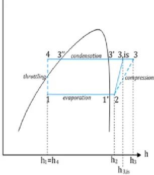
Figure 4-1 Thermodynamic vapor compression cycle in log(p)-h diagram ... 9
Figure 4-2 Heat pump system schematic ... 9
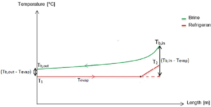
Figure 4-3 Temperature profile in the evaporator ... 10
Figure 4-4 Temperature profile in the condenser ... 13
Figure 4-5 Matlab model algorithm flow chart... 15
Figure 4-6 Matlab heat pump model graphical user interface ... 16
V
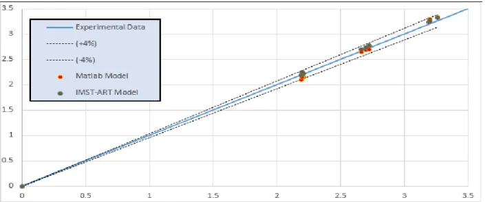
Figure 4-8 Heating capacity (kW) from experimental data vs. heat pump models ... 17
Figure 4-9 Compressor power (kW) from experiment vs. heat pump models ... 17
Figure 4-10 Condensation temperature (°C) from experimental data vs. heat pump models ... 18
Figure 6-1 Sensitivity ratioFDD model algorithm ... 23
Figure 6-2 Graphical user interface for sensitivity ratio method based FDD model ... 24
Figure 6-3 Fault type and level detected using sensitivity ratio method for operation conditions W30B0, W40B0 and W50B0 ... 25
Figure 7-1 Original data matrix ... 26
Figure 7-2 Eigenvectors and eigenvalues ... 27
Figure 7-3 Principle components analysis algorithm... 28
Figure 7-4 The eigenvalues for each eigenvector ... 29
Figure 7-5 Percentage of the variance along each eigenvector ... 29
Figure 7-6 𝑷𝑪𝟏𝒔𝒕 and 𝑷𝑪𝟐𝒏𝒅 projections of operation conditions data ... 30
Figure 7-7 𝑷𝑪𝟐𝒏𝒅 and 𝑷𝑪𝟑𝒓𝒅 projection of faulty data groups centers in operation condition W30B0 ... 31
Figure 7-8 Operation condition clusters in 𝑷𝑪𝟏𝒔𝒕 and 𝑷𝑪𝟐𝒏𝒅 dimensions ... 32
Figure 7-9 Example for operation conditions, clusters, CR, DC and OCCR ... 33
Figure 7-10 Example for fault type and classification concept ... 34
Figure 7-11 PCA FDD model algorithm ... 35
Figure 7-12 Graphical user interface for PCA method based FDD model ... 36
Figure 7-13 PCA FDD model accuracy for each operation condition ... 36
Figure 7-14 FPF values for condenser (low, medium and high) fouling results at W30B0 ... 37
Figure A-1 Fault type and level detected using sensitivity ratio method for operation conditions W30B-5, W40B-5 and W50B-5 ... i
Figure A-2 Fault type and level detected using sensitivity ratio method for operation conditions W30B5, W40B5 and W50B5 ... i
Figure A-3 Sketch showing the orthogonal distance d between a point and a line ... ii
Figure A-4 Parameters used in original matrix ... iii
Figure A-5 The PCA results in 10 eigenvectors in 10 columns (principle components), each row is the coeficient value to be multiplied by the original parameters values ... iii
Figure A-6 The PCA results in 10 eigenvalues to represent how much variance is described along each eigenvector (principle component) ... iii
List of Tables
Table 4-1 Operating conditions for the heat pump unit used for the experinetal data ... 8Table 5-1 Fault types, fault simulation and fault levels ... 19
Table 5-2 Faulty characteristics of the heat pump parameters ... 20
Table 6-1 Absolute value of error between Matlab model and experiment data ... 21
Table 6-2 Suggested tolerances for the parameters' residuals for each operation condition ... 22
Table 6-3 The sensitive and insensitive parameters and for each fault ... 22
VI
Nomenclature
𝑨 Area [m²]
𝑮𝑯𝑬 Greenhouse emissions [-]
𝑭𝑫𝑫 Fault detection and diagnosis [-]
𝑺𝑭𝑫𝑫 Smart fault detection and diagnosis [-]
𝑫𝑯𝑾 Domestic hot water [-]
𝑬𝒙𝒑. 𝑽𝒂𝒍𝒗𝒆 Expansion valve [-]
𝑬𝒍𝒆𝒄. 𝑴𝒐𝒕𝒐𝒓 Electrical motor [-]
𝑸̇𝟏 Heating capacity of the heat pump [kW]
𝑸̇𝟐 Cooling capacity of the heat pump [kW]
𝑾̇ Compression work input to the cycle [kW]
𝑾̇𝒊𝒔 Isentropic compression work input to the cycle [kW]
𝒎̇𝒘 Mass flow rate of water [kg/s]
𝒎̇𝒃 Mass flow rate of brine [kg/s]
𝒎̇𝒓𝒆𝒇 Mass flow rate of refrigerant [kg/s]
𝑪𝑶𝑷𝟏 Coefficient of performance in the heating mode [-]
𝑪𝑶𝑷𝟏 Coefficient of performance in the cooling mode [-]
PCA Principle component analysis [-]
BPHE Brazed plate heat exchanger [-]
𝑻 Temperature [°C]
𝑻𝒃,𝒊𝒏 Brine inlet temperature to evaporator [°C]
𝑻𝒃,𝒐𝒖𝒕 Brine outlet temperature to evaporator [°C]
𝑻𝒘,𝒊𝒏 Water inlet temperature to condenser [°C]
𝑻𝒘,𝒐𝒖𝒕 Water outlet temperature to condenser [°C]
𝑻𝒄𝒐𝒏𝒅 Condensation temperature [°C]
𝑻𝒆𝒗𝒂𝒑 Evaporation temperature [°C]
𝒉 Specific enthalpy [kJ/kg]
𝒔 Specific entropy [kJ/kg.K]
𝑽̇𝒔𝒘𝒆𝒑𝒕 Swept volume [m3/s]
𝒄𝒑 Specific heat capacity [kJ/kg.K]
𝑼𝒆𝒗𝒂𝒑 Overall heat transfer coefficient of the evaporator [kJ/m².K]
𝑨𝒆𝒗𝒂𝒑 Heat transfer area of the evaporator [m²]
𝑳𝑴𝑻𝑫𝒆𝒗𝒂𝒑 Logarithmic mean temperature difference over the
evaporator
[°C]
𝑼𝒄𝒐𝒏𝒅 Overall heat transfer coefficient of condenser [kJ/m².K]
𝑨𝒄𝒐𝒏𝒅 Heat transfer area of the condenser [m²]
𝑳𝑴𝑻𝑫𝒄𝒐𝒏𝒅 Logarithmic mean temperature difference over the condenser [°C]
𝑲𝑷𝑰 Key performance indicators [-]
𝑴 Molar mass [kg/mol]
𝐏𝒓𝒆𝒅𝒖𝒄𝒆𝒅 Reduced pressure [-]
𝒒̈ Heat flux [kW/m²]
VII
𝑹𝒆 Rynolds number [-]
𝑷𝒓 Prandtl number [-]
𝐝𝒆 Hydraulic diameter [m]
𝑮 Mass flux [kg/s.m²]
𝐮𝒎 Channel flow velocity [m/s]
𝑽̇𝒔𝒘𝒆𝒑𝒕 Swept volume [m3/s]
𝑷𝒓𝒂𝒕𝒊𝒐 Pressure ratio over the compressor [-]
𝒈 Gravitational acceleration [m/s²]
𝜟𝑻𝒆𝒗𝒂𝒑 Difference between evaporation temperatures before and after the fault
[°C]
𝜟𝑻𝒄𝒐𝒏𝒅 Difference between condensation temperatures before and after the fault [°C]
𝜟𝑻𝒘 Difference between water inlet and outlet temperatures [°C] 𝜟𝑻𝒃 Difference between brine inlet and outlet temperatures [°C]
𝜟𝑻𝒔𝒖𝒃 Sub-cooling temperature difference [°C]
𝜟𝑻𝒔𝒖𝒑 Super-heating temperature difference [°C]
𝑻𝒅𝒊𝒔 Compressor discharge temperature [°C]
𝑬𝒄𝒐𝒎𝒑 Compressor power input [kW]
𝑭𝑹𝒇𝒂𝒖𝒍𝒕 Fault sensitivity ratio [-]
𝑷𝑰 Performance indicator [°C or kW]
𝑷𝑹 Performance indicator residual [°C or kW]
𝑿𝒏×𝒎 Original training data matrix [-]
𝑿𝒏𝒐𝒓𝒎𝒂𝒍𝒊𝒛𝒆𝒅𝒏×𝒎 Normalized training data matrix [-]
𝑽𝒏×𝒎 Eigenvectors matrix [-]
𝑫𝒏×𝒎 Eigenvalues matrix [-]
𝑨𝒏×𝒌 Data matrix of original training data projection into the
principle components
[-]
𝑽𝒆𝒙𝒑,𝒊 Eigenvalue ratio to summation of all eigenvalues [-]
𝑪𝑪 Cluster center [-]
𝑪𝑹 Cluster radius [-]
𝑫𝑪 Distance between a point and a center of cluster [-]
𝑶𝑪𝑪𝑹 Operation condition cluster ratio [-]
𝑶𝑫 Orthogonal distance [-]
𝑷𝑷 Point projection on fault line segment [-]
𝑷𝑫 Distance from point projection and fault line segment start [-]
𝑭𝑫 Fault segment length [-]
𝑭𝑳𝑹 Fault level ratio [-]
𝑭𝑷𝑭 Fault probability factor [-]
𝑭𝟏 Condenser fouling [-] 𝑭𝟐 Evaporator fouling [-] 𝑭𝟑 Water underflow [-] 𝑭𝟒 Water overflow [-] 𝑭𝟓 Refrigerant undercharge [-] 𝑭𝟔 Refrigerant overcharge [-]
VIII
𝑭𝟕 Brine underflow [-]
𝑭𝟖 Brine overflow [-]
𝑭𝟗 Expansion valve malfunction [-]
𝑭𝟏𝟎 Compressor malfunction [-]
Greek Characters
𝛂 Convictive heat transfer coefficient [kJ/m².K]
𝝀 Thermal conductivity [W/m.°C]
𝝆 Density [kg/ m³]
𝝁 Dynamic viscosity [Pa/s]
𝝑𝒆𝒗𝒂𝒑,𝒊𝒏 Difference between the brine inlet temperature and
evaporation temperature
[°C]
𝝑𝒆𝒗𝒂𝒑,𝒐𝒖𝒕 Difference between the brine outlet temperature and evaporation temperature
[°C]
𝝑𝒅𝒆𝒔 Difference between the discharge temperature and water outlet temperature
[°C]
𝝑𝒄𝒐𝒏𝒅,𝒐𝒖𝒕 Difference between the condensation temperature and water pinch point temperature
[°C]
𝝑𝒄𝒐𝒏𝒅,𝒊𝒏 Difference between the condensation temperature and water temperature corresponding to refrigerant liquid saturation point
[°C]
𝝑𝒔𝒖𝒃 Difference between the condenser outlet temperature and water inlet temperature
[°C]
𝛈𝐢𝐬 Compressor isentropic efficiency [-]
𝛈𝐬 Compressor volumetric efficiency [-]
Ʃ Covariance matrix [-]
Subscription
𝟏 Expansion valve outlet / evaporator inlet in refrigerant cycle [-] 𝟐 Evaporator outlet / compressor inlet in refrigerant cycle [-] 𝟑 Compressor outlet / condenser inlet in refrigerant cycle [-] 𝟑𝒊𝒔 Ideal compressor outlet / condenser inlet in refrigerant cycle [-] 𝟒 Condenser outlet / expansion valve inlet in refrigerant cycle [-]
𝟓 Evaporator inlet on the brine side [-]
𝟔 Evaporator outlet on the brine side [-]
𝟕 Condenser inlet on the water side [-]
𝟖 Condenser outlet on the water side [-]
′′ Saturated liquid line [-]
′ Saturated vapor line [-]
𝒊𝒏,𝒔𝒆𝒏𝒔 insensitive [-]
𝒔𝒆𝒏𝒔 sensitive [-]
𝑻 Transpose of a matrix [-]
𝑷𝑪𝟏𝒔𝒕 Data point coordinate on first principle component [-]
𝑷𝑪𝟐𝒏𝒅 Data point coordinate on second principle component [-]
1
1 Introduction
In Sweden alone, there are approximately more than one million heat pumps already installed. In the current single family houses, the heat pump market share is about 50% while it is nearly 90% in the newly built ones (Forsen, 2012). Therefore, small improvements on the heat pump performance could lead to a significant amount of savings in energy usage thus reducing the Green House Emissions to a large extent.
In heat pumps systems, usually manufacturer set certain operation standards to ensure the best possible performance. But in the installed heat pump systems, it is not unusual for them to operate in different conditions than the standard ones set by the manufacturer. Such a deviation could cause efficiency degradation in the heat pump systems. This deviation can be caused by initial installation error, control devices malfunction or components wearing out over time consequently leading to an overall performance degradation in the heat pump system or ultimately causing components or system failure.
Moreover, over the past recent years, significant amount of failure and faults reports in heat pumps systems were filed to heat pump manufacturers and insurance companies. Among these failure and fault reports, a sizable amount were a related to inaccurate installation or fault misdiagnosis by the servicemen (Madani et al., 2014). Such a mistake by the servicemen could lead to heat pump system performance degradation, system failure or replacement of unnecessary component. These would lead to needless avoidable additional costs on the manufacturers, insurance companies and end-costumer.
To avoid such costs, a proposed solution is to automate fault detection and diagnosis (FDD) process. Furthermore, producing a Smart Fault Detection and Diagnosis (SFDD) system connected to the heat pump that can assist the servicemen during the installation, operation and maintenance processes to reduce misdiagnosis and assure the highest performance in the heat pump systems. Therefore, reducing or avoiding any unnecessary additional costs such as system performance reduction, component replacement, unneeded visual inspection and system down-time for maintenance.
1.1 System Boundaries
To set up SFDD system it is important to set the system boundary levels in which the SFDD would be considered to operate within. Fault detection in heat pump systems can be viewed from four different boundaries as follows (Lundqvist, 2010):
1. Heat pump unit level which includes the heat pump components all together such as evaporator, compressor, condenser, expansion valve and refrigerant.
2. Heat pump system level which include the heap pump unit components together with heat source, heat sink, axillary heater and circulating pumps of brine and water.
3. Building system level which include the heat pump system together with building specifications, thermal insulation, domestic hot water (DHW) system, thermal solar collectors, inhabitant habits, etc.
2
Figure 1-1 System Boundaries Layout
Different systems’ boundaries for heat pump system (Madani et al., 2014)
1.2 Heat Pump Working Principle
Heat pumps are one of the applications of vapor compression thermodynamic cycle (also called refrigeration cycle) which can be used for both cooling and heating applications. The cycle consists of two pressure levels where there are a heat sink and heat source on the high and low pressure levels respectively. The heat pump cycle mainly consists of evaporator, compressor, condenser and expansion valve as shown in Figure 1.2. In the heat pump the main interest is in the output heating capacity (𝑸̇𝟏) of the cycle to the heat sink. The heat pump mainly convey energy using a
working fluid from the heat source (𝑸̇𝟐) at the relatively low pressure (and low temperature) level to the heat sink high pressure (and high temperature) level by adding additional electrical work through a compressor (𝑾̇). The cycle starts when the working fluid is heated and vaporized while energy is transferred from the heat source to the working fluid using a secondary fluid flow (brine) in the evaporator and then then compressed to a higher pressure level. Then the working fluid is cooled down and its energy is transferred to the secondary fluid flow (water) in the heat sink in the condenser. After that, the working fluid run through the expansion valve thus its pressure level is reduced and it starts to evaporate again in the evaporator and the cycle continue to repeat itself (Granryd et al., 2011).
3
Figure 1-2 Heat Pump Schematic
This schematic shows the main component of a heat pump
In case of an adiabatic system, the system can be represented by the energy balance equation below see Eq. [1].
𝑄̇1 = 𝑄̇2 + 𝑊̇ [1]
In the heating mode and cooling mode, the heat pump system overall performance is evaluated by the coefficient of performance (𝐶𝑂𝑃1) and (𝐶𝑂𝑃2) respectively. The heating and cooling coefficients of performance are calculated as shown in Eq. [2] and Eq. [3] respectively
𝐶𝑂𝑃1 = 𝑄̇1/𝑊̇ [2]
𝐶𝑂𝑃2 = 𝑄̇2/𝑊̇ [3]
1.3 Background in Fault Detection and Diagnosis
In the area of fault detection and diagnosis in heat pumps, the aim is to automate the inspection procedure that is done by the servicemen. This help them to find out about faults in the system in an early stage and diagnose them correctly thus avoiding major system performance degradation or system failure (Vecchio, 2014). Fault detection and diagnosis systems were initially used in
4
very critical system such as nuclear related application and power plant. But with technology development along the years, enhanced hardware computational capabilities and the reduction in their prices, it became more feasible to integrate fault detection and diagnosis procedures in less critical applications such as automotive (Svärd, 2012) and (Suwatthikul, 2010), industrial systems (Roth, 2010) and heat pump systems to ensure the highest performance possible and reduce losses as possible.
1.3.1 Fault detection and diagnosis methods
For typical operation and maintenance procedures involving FDD system, there are four main steps need to be followed. Fault detection, in which the system evaluates the operation condition and detects if there is any unusual activity (fault). If any abnormal activity is detected, the system runs the diagnosis system to isolate the fault and identify the location of the problem. Following the issue identification, an evaluation of the size of the issue and how significant its impact on the system performance. Finally, based on the fault evaluation results, a decision will be made as system shut down, control reconfiguration, repair request or continue the operation in case of an insignificant effect of the fault. Mainly the first two steps of this procedure form the fault detection and diagnosis model (Katipamula and Brambley, 2005), (Isermann and Balle, 1997).
In literature, there are different methods for fault detection and diagnosis that can be summarized into three categories. These categories are quantitative based methods, qualitative based methods and processed history based methods. The methods were compared based on several desired characteristics in fault detection and diagnosis methods such as response quickness, ability to distinguish between different faults, diagnosis accuracy, and adaptability to change in input parameters or internal structure and modeling requirements. Eventually, advantages, disadvantages and most suited application of each different FDD method were discussed (Venkat et al., 2003c), (Venkat et al., 2003a), (Venkat et al., 2003b), (Katipamula and Brambley, 2005). A summary of FDD methods is shown in Figure 1.3.
5
Figure 1-3 Fault detection and diagnosis methods (Katipamula and Brambley, 2005)
Likewise, in (Zhang and Jiang, 2008), the fault detection and diagnosis methods were categorized into two main categories, model based and data based methods. Then each one is divided into quantitative and qualitative approaches.
1.3.2 Fault Detection and Diagnosis in Heat Pumps
Regarding heat pump FDD, in previous literature, several FDD models have been developed for different applications and different boundary levels. For instances on the component boundary level, a FDD model for leakage detection in check valves and reversing valves in heat pumps operating in cooling mode was developed by (Li. and Braun, 2009). The decoupling method was used in the FDD model. This method connects certain physical feature with certain fault through a mathematical relationship. Thus it can distinguish between faults.
On the heat pump unit level, several FDD models were developed using different techniques. In the year 2000, (Chen. and Braun., 2000) have suggested a simple fault detection and diagnosis method for packaged air conditioners. His model consisted of black box regression model of the heat pump and two proposed methods for FDD model. The first method, sensitivity ratios were introduced between two different parameters. Each ratio is uniquely sensitive to a certain fault. The second is simple rule based FDD method consisting of temperature limit checking procedure. These methods are to be used in a steady state fault detection.
In 2002, D. Zogg (Zogg, 2002) developed two FDD systems for heat pump units, FuzzyWatch and HeatWatch. FuzzyWatch system identifies the heat pump characteristics using black-box and gray-box models. Then, in the fault diagnosis process, statistical, fuzzy logic and neural networks techniques were used. Training data for fault free and faulty conditions were obtained from two test benches. In the training stage, several hard and soft clustering methods were considered. Each fault was represented by a cluster during the training phase and a membership grade was
6
introduced which evaluates the measured data and identifies which cluster (fault) they belong to. HeatWatch system calculates the heat pump physical characteristics and parameters using a steady state model. The system is initialized by loading fault free data of the heat pump parameters to act as reference values. Then, the fault diagnosis process is based on finding the deviation of the calculated parameters from the reference values. The change in certain parameter or characteristic in the heat pump is interpreted as a certain fault.
1.3.3 Motivation
In the literature review above, most fault detection and diagnosis methods developed involve heat pump modeling and FDD modeling. In heat pump modeling, in most cases data driven regression black box model of the heat pump were obtained. Such approaches require large amount of measurements data for training. In addition, the heat pump model is built for a specific heat pump unit and specific range of operation conditions and cannot be used for other units or operation conditions outside the training data range. Likewise, in the FDD model development, in most literature, either simple rule based limit checking or data-driven black-box models were developed. Rule based methods are usually flexible and easy to implement, but lack of fault isolation in fault diagnosis. Data driven models are rather accurate and can distinguish between faults, but inflexible to be used for other types of heat pumps (e.g., ground source heat pumps), demands high computational hardware requirements and usually requires a large amount of training data for fault free and faulty conditions that can be either costly or hard to obtain.
Among the several types of heat pumps (e.g. air to air, air to water and brine to water heat pumps), the brine to water heat pump is the most expensive one. Therefore, implementing a FDD system would be more feasible and convenient in such a system. Thus, ground source brine to water heat pump was considered in this thesis.
2 Objectives
The objectives of this thesis is to develop two fault detection and diagnosis methods for ground source brine to water heat pumps on the unit boundary level including evaporator, compressor, condenser and expansion valve. In addition to the heat pump unit, the brine and water pumps components from the heating system boundary level are included. The main aims of this thesis are as following:
1. Build a fault detection and diagnosis model for steady state operation conditions using sensitivity ratio with semi-empirical heat pump model to different heat pumps types. 2. Build a fault detection and diagnosis model for steady state operation using principle
component analysis (PCA) in the FDD modeling to enhance the fault diagnosis accuracy. 3. Both methods require simple temperature data measurements to be developed and run. This
is to reduce the implementation cost and to be more convenient for the customer. 4. Relativity low computational and hardware requirements to run the tool.
7
3 Methodology
This thesis was carried out in the following phases:
i. Literature review of FDD methods and selecting the ones to be considered in this thesis. ii. Heat pump semi-empirical modelling using Matlab and IMST-ART software and cross
validate the models with experimental data.
iii. Faults simulation in the heat pump model using IMST-ART and trend analysis. iv. Identifying key performance indicators by performing trend analysis of the system
variables.
v. Building FDD model using sensitivity ratio method and model validation.
vi. Obtaining mathematical key performance indicators using principle component analysis (PCA) method.
vii. Building FDD model using PCA based fault clustering method.
The work in this thesis started by a literature review of FDD methods in different fields followed by a review of the FDD techniques that have been developed for FDD in different types of heat pumps, then choosing the FDD method to be considered for modelling.
For FDD modelling, a heat pump model was developed first to represent the reference line for a fault free operation. In this step a semi-empirical vapor compression heat pump cycle model based on the physical principles and experimental data obtained form an installed ground source heat pump unit operating in different temperature ranges (see Table 4.1). Two heat pump models are built using Matlab and IMST-ART software. The results from both models are validated against the experimental data.
After obtaining the heat pump models, IMST-ART model is used to simulate different faults in the heat pump unit components in addition to the brine and water pumps. Then, trend analysis is conducted to investigate the effect of each fault on different system variables such as temperatures, pressures, heat transfer coefficients and coefficient of performance.
In the next step, after fault trend analysis, certain key performance indicators (KPI) are selected that uniquely sensitive for each fault. There are two different types KPIs used in this thesis, physical and mathematical. Physical KPIs are chosen based on the trend analysis whereas the mathematical ones are calculated using PCA.
Furthermore, physical KPIs are used in developing FDD model using sensitivity ratio method whereas mathematical KPIs are used to build FDD model based on clustering method. Both models are tested using new generated data for the different faults using the IMST-ART model.
Finally, for both FDD models, user friendly interfaces were developed that make it more convenient to handle by any technician or serviceman.
8
Figure 3-1 Thesis structure and methodology flow chart of this thesis
4 Heat Pump Modelling
The heat pump unit considered in this work consist of four main components, evaporator, compressor, condenser and an expansion valve. Both evaporator and condenser are Brazed Plate Heat Exchangers (BPHE), the compressor is a hermetic scroll type and the expansion device is thermostatic valve. The main working fluid (refrigerant) is R410A whereas the secondary working fluids are water and brine (mixture of water and ethyl alcohol with 29% fixed concentration) in the condenser and evaporator respectively.
A semi-empirical model was built based on the first principles using empirical measurements obtained from an heat pump operating in nine operating conditions (see Table 4.1). Each component of the heat pump unit is modeled based on the physical principles of thermodynamics, energy and mass balance. The related governing physical relationship for each component will be discussed later in this chapter.
Table 4-1 Operating conditions for the heat pump unit used for the experinetal data
Heat Source Temperature (𝑻𝟓) [°C] Heat Sink Temperature (𝑻𝟕) [°C]
-5 30 40 50 0 30 40 50 5 30 40 50
9
Connecting the thermodynamic cycle with the physical components of the heat pump system, Figure 4.1 and Figure 4.2 show the thermodynamic cycle of the heat pump unit and the schematic of the heat pump system. Number 1, 2, 3 and 4 on both figures represent the conditions at the inlets of evaporator, compressor, condenser and expansion valve respectively on the refrigerant side.
Figure 4-1 Thermodynamic vapor compression cycle in log(p)-h diagram
10
In Figure 4.2, numbers 5 and 6 represent the conditions at evaporator inlet and outlet respectively on the brine side. Whereas numbers 7 and 8 represent the conditions at condenser inlet and outlet respectively on the water side.
4.1 Evaporator Modeling
In this work the evaporator considered is BPHE with counter flow. Typical temperature profile for such evaporator is shown in Figure 4.3.
Figure 4-3 Temperature profile in the evaporator
The evaporator sub-model has been developed by applying the energy balance equations to describe the heat transfer (𝑸̇𝟐) from the heat source (the brine) to the refrigerant. This process can be described the below mentioned equations (see Eq. [4], [5] and [6]).
𝑄̇2 = 𝑚̇𝑟𝑒𝑓 (ℎ2− ℎ1 ) [4]
𝑄̇2 = 𝑚̇𝑏∗ 𝑐𝑝𝑏𝑟𝑖𝑛𝑒 ∗ (𝑇𝑏,𝑖𝑛− 𝑇𝑏,𝑜𝑢𝑡 ) [5]
𝑄̇2 = 𝑈𝐴𝑒𝑣𝑎𝑝∗ 𝐿𝑀𝑇𝐷𝑒𝑣𝑎𝑝 [6]
For heat transfer in BPHE, (Claesson, 2004) compared empirical data and theoretical values of the logarithmic mean temperature difference (LMTD) and found that the correction factor yield to 1 (which means approximately an error value close to zero) when the LMTD value increase. He concluded that LMTD approach fairly accurate to be used for moderate and high LMTD values. Therefore, an additional relationship can be added to describe the heat transfer over the evaporator as shown in Eq. [6].
11
The LMTD for the evaporator can be calculated by Eq. [7]
𝐿𝑀𝑇𝐷𝑒𝑣𝑎𝑝 =
(𝑇𝑏,𝑖𝑛 − 𝑇𝑒𝑣𝑎𝑝) − (𝑇𝑏,𝑜𝑢𝑡− 𝑇𝑒𝑣𝑎𝑝)
ln [(𝑇𝑏,𝑖𝑛− 𝑇𝑒𝑣𝑎𝑝) (𝑇𝑏,𝑜𝑢𝑡− 𝑇𝑒𝑣𝑎𝑝)]
[7]
By neglecting the heat transfer resistance in the wall between the refrigerant and the brine in the evaporator, the overall heat transfer coefficient can be estimated by Eq. [8].
1 𝑈𝑒𝑣𝑎𝑝,𝑡𝑜𝑡 = 1 α𝑒𝑣𝑎𝑝,𝑟𝑒𝑓+ 1 α𝑏𝑟𝑖𝑛𝑒 [8]
In literature, many correlation has been suggested to calculate the evaporation heat transfer coefficient in BPHX. However, according to (Claesson, 2004), the most accurate correlation that estimate the evaporation heat transfer coefficient in BPHE is Cooper’s pool boiling correlation shown in Eq. [9].
α𝑒𝑣𝑎𝑝,𝑟𝑒𝑓 = C1∗ P𝑟𝑒𝑑𝑢𝑐𝑒𝑑C2∗ (−log
10 P𝑟𝑒𝑑𝑢𝑐𝑒𝑑)C3∗ 𝑀C4∗ 𝑞̈ C5 [9]
Where P𝑟𝑒𝑑𝑢𝑐𝑒𝑑 is the ratio of the evaporation pressure over the critical pressure, M the molar
mass, 𝑞̈ is the heat flux over the evaporator and C1to C5 are constants that are determined by fitting empirical data measurements from the evaporator operating in the different operating conditions (see Table 4.1).
The heat transfer coefficient on the brine side is calculated using Bogaert and Bölcs correlation for single phase flow (Eq. [10] and Eq. [11]).
𝑁𝑢 = B1∗ 𝑅𝑒B2∗ 𝑃𝑟13𝑒 6.4 𝑃𝑟+30 [10] α𝑏𝑟𝑖𝑛𝑒 = 𝑁𝑢 ∗ 𝜆 d𝑒 [11]
Where d𝑒 value can be estimated to same as the spacing between plates in BPHX (Claesson, 2004), Reynolds and Prandtl number are calculated from Eq. [12] and [13] respectively.
𝑅𝑒 = 𝜌 ∗ u𝑚∗ d𝑒 𝜇 = 𝐺 ∗ d𝑒 𝜇 [12] 𝑃𝑟 = c𝑝∗ 𝜇 𝜆 [13]
B1to B2 in Eq. [10] are constants that are determined by fitting empirical data measurements from the evaporator operating in the different operating conditions (see Table 4.1).
12
4.2 Compressor Modelling
In this work, a hermetic scroll fixed speed (2900 rpm or 50 Hz) compressor with swept volume (𝑉̇𝑠𝑤𝑒𝑝𝑡) of 0.001925 (m3/s) (Emerson_Climate_Technologies, 2015) is used. In the ideal case of
an isentropic compression, the ideal compressor discharge enthalpy (ℎ3,𝑖𝑠) would equal the actual
one (ℎ3). In reality though, that is not the case. Due to losses during converting electrical power input into thermal power in the refrigerant, an isentropic efficiency (ηis) is defined (Eq.16). The compressor sub-model has been developed by applying the energy balance equations to describe the compressor power (𝑊̇) input to the refrigerant. This process can be described by Eq. [14] and Eq. [15]. 𝑊̇𝑖𝑠= 𝑚̇𝑟𝑒𝑓∗ (ℎ3,𝑖𝑠− ℎ2) [14] 𝑊̇ = 𝑚̇𝑟𝑒𝑓 ∗ (ℎ3− ℎ2) [15] ηis = h3,is− h2 h3− h2 [16]
According to (Granryd et al., 2011), the mass flow rate of refrigerant can be estimated by Eq. [17].
𝑚̇𝑟𝑒𝑓 = 𝜌2 ∗ 𝑉̇𝑠𝑤𝑒𝑝𝑡∗ 𝜂𝑠 [17]
For calculating the isentropic and volumetric efficiencies, correlations provided by manufacturer are used as shown in Eq. [18] and Eq. [19] respectively.
ηis = 𝑎0∗ 𝑃𝑟𝑎𝑡𝑖𝑜 𝑎1 − 𝑎 2 𝑃𝑟𝑎𝑡𝑖𝑜𝑎3 + 𝑎 4 [18] ηs = 𝑏0∗ 𝑃𝑟𝑎𝑡𝑖𝑜+ 𝑏1 [19]
The constants 𝑎0, 𝑎1, 𝑎2, 𝑎3, 𝑎4, 𝑏0 and 𝑏1 are determined by fitting manufacturer data of isentropic and volumetric efficiencies obtain over a wide range of operation condition
4.3 Condenser Modelling
Similar to the evaporator, the condenser considered is BPHE with counter flow. Typical temperature profile for such evaporator is shown in Figure 4.4.
13
Figure 4-4 Temperature profile in the condenser
Like the evaporator, the condenser sub-model has been developed by applying the energy balance equations to describe the heat transfer (𝑸̇𝟏) from the heat sink (the water) to the refrigerant. This process can be described the below mentioned equations (see Eq. [20], [21] and [22]).
𝑄̇1 = 𝑚̇𝑟𝑒𝑓 (ℎ3− ℎ4 ) [20]
𝑄̇1 = 𝑚̇𝑤 ∗ 𝑐𝑝𝑤𝑎𝑡𝑒𝑟∗ (𝑇𝑤,𝑜𝑢𝑡− 𝑇𝑤,𝑖𝑛 ) [21]
𝑄̇1 = 𝑈𝐴𝑡𝑜𝑡∗ 𝐿𝑀𝑇𝐷𝑡𝑜𝑡 [22]
According to (Granryd et al., 2011), for the condensation phase in the condenser the LMTD can be calculated by Eq. [23]
𝐿𝑀𝑇𝐷𝑐𝑜𝑛𝑑 = 𝜗𝑐𝑜𝑛𝑑,𝑖𝑛− 𝜗𝑐𝑜𝑛𝑑,𝑜𝑢𝑡 ln [𝜗𝜗𝑐𝑜𝑛𝑑,𝑖𝑛
𝑐𝑜𝑛𝑑,𝑜𝑢𝑡]
[23]
By neglecting the heat transfer resistance in the wall between the refrigerant and the water in the condenser, the overall heat transfer coefficient can be estimated by Eq. [24].
1 𝑈𝑐𝑜𝑛𝑑,𝑡𝑜𝑡 = 1 α𝑟𝑒𝑓+ 1 α𝑤𝑎𝑡𝑒𝑟 [24]
The heat transfer coefficient for doubles phase flow can be estimated using the classic Nusselt theory for the condensation phase as in Eq. [25].
α𝑐𝑜𝑛𝑑,𝑟𝑒𝑓∗ 1 𝜆3′′∗ [ 𝜇3′′ 𝜌3′′∗ (𝜌 3′′− 𝜌3′) ∗ 𝑔] B5 = B3∗ 𝑅𝑒𝐵4 [25]
14
B3, B4 and B5 in Eq. [25] are constants that are determined by fitting empirical data measured from
the condenser operating in the different operating conditions (see Table 4.1).
Similar to the evaporator, for calculating the heat transfer coefficient for single phase flow in the condenser, Bogaert and Bölcs correlation can be used as previously mentioned in Eq. [10]. The constant B1 and B2 are adapted by fitting empirical data measured for the de-superheating and
sub-cooling zones on the refrigerant side as well as the single phase flow on the water side over different operating conditions (see Table 4.1)
4.4 Expansion Valve Modelling
In this work, the expansion device used is thermostatic valve, following the first principle of thermodynamics shown in Eq. [26].
𝛥ℎ + 𝛥𝑒𝑘+ 𝛥𝑒𝑝 = 𝑞̈ − 𝑤 [26]
Where 𝛥ℎ is the enthalpy change in (J/kg), 𝛥𝑒𝑘 the kinetic energy change (J/kg), 𝛥𝑒𝑝 the potential energy change (J/kg), q the exchanged specific heat (J/kg) and w is the required work for the expansion process. The assumptions are made that there is no change in kinematic nor potential energy during the expansion process as well as no work needed to perform the expansion and no heat exchanged with the surroundings. Therefore, the throttling is considered an isenthalpic process, and thus ℎ1 = ℎ4. Based on the empirical data, the expansion valve is assumed to provide a certain superheat temperature depending on the operation condition in fault free case.
4.5 Matlab Model
The main aim of this model to be used as a reference line later in the FDD model. Therefore, a semi-empirical steady state fault free heat pump model was developed using Matlab. The model was built based on solving a system of equations using energy balance equations applied on the four components, evaporator, compressor, condenser and expansion valve as mentioned earlier. From the optimization toolbox in Matlab, lsqnonlin function was used to solve the equation system. lsqnonlin is function that can solve nonlinear least-squares curve fitting problems while providing the option to set lower and upper boundaries for the assigned variables (Mathworks, 2015b).
The model inputs values are 𝑇5, 𝑇7, 𝑚̇𝑤, 𝑚̇𝑏, 𝐴𝑒𝑣𝑎𝑝,𝑡𝑜𝑡, 𝐴𝑐𝑜𝑛𝑑,𝑡𝑜𝑡 and 𝑉̇𝑠𝑤𝑒𝑝𝑡. Then educated initial
guesses are generated for 𝑇𝑒𝑣𝑎𝑝, 𝑇𝑐𝑜𝑛𝑑, 𝛥𝑇𝑠𝑢𝑝𝑒𝑟ℎ𝑒𝑎𝑡, 𝛥𝑇𝑠𝑢𝑏𝑐𝑜𝑜𝑙𝑖𝑛𝑔. Then initial guesses for the rest of the variables are calculated from a simple regression correlations using the experimental data. Then, an iterative procedure starts in the model and after each iteration the variables are set with new values. The model keep iterating until the maximum preset number of iteration is reached or the changes between the variables’ previous and the values are less than a pre-specified tolerance (see Figure 4.5). The thermodynamic properties are taken from CoolProp. Coolprop is a C++ library that can be added to Matlab for fluid properties (CoolProp, 2015).
15
Figure 4-5 Matlab model algorithm flow chart
After building the Matlab code, a graphical user interface is created to facilitate the use of the model (see Figure 4.6).
16
Figure 4-6 Matlab heat pump model graphical user interface
4.6 IMST-ART Model
A second steady state heat pump model was developed using the software IMST-ART developed by the Polytechnic University of Valencia for vapor compression cycles. The model inputs are shown in Figure 4.7. For more details about the correlations used in the software, please refer to the guide (Universidad_Politécnica_Valencia, 2013).
Figure 4-7 IMST-ART interface and model input summary 4
17
4.7 Heat Pump Model Validation
The significance of the heat pump model is that it predicts the normal operation conditions for the unit which can be used later on as a reference line for the FDD model. The relevant parameters are coefficient of performance, heating capacity, compressor power and temperatures across the refrigerant and both secondary working fluids. Both Matlab and IMST-ART model were cross validated with the experimental data at the operation conditions mentioned in Table 4.1. The above mentioned variables were cross validated found to be within ±7% marginal error compared to experimental data. In the following figures, heating capacity, compressor power and condensation temperature are displayed as examples of the parameters validation in Figure 4.8, Figure 4.9 and Figure 4.10. For developing FDD model the
Figure 4-8 Heating capacity (kW) from experimental data vs. heat pump models
18
Figure 4-10 Condensation temperature (°C) from experimental data vs. heat pump models
5 Fault Analysis
In previous literature, a review of the most common and costly faults in heat pumps system were made (Madani et al., 2014). The possible faults are dependent on the boundary level considered. The boundary level considered in this work is the heat pump unit consisting of evaporator, compressor, condenser and expansion valve in addition to the secondary fluid pumps. During the operation of a heat pump unit, possible problems might occur. When such a fault propagates, the system and component characteristics deviate from the nominal operation conditions. Therefore, the knowledge of the faulty system characteristics is needed to develop FDD model. Such data can be obtained either from an experimental set up or by simulation software. In this work the heat pump unit faulty characteristics were obtained by fault simulation using IMST-ART software.
5.1 Faults Simulation
After validation the heat pump models, IMST-ART model was used for fault simulation. In a heat pump unit, seven common faults are considered in this simulation.
- Evaporator fouling (blockage). - Condenser fouling (blockage). - Compressor malfunction (wear).
- Expansion valve malfunction (too high superheating temperature). - Water cycle (leakage in pipes or water pump malfunction).
- Brine cycle (leakage in pipes or brine pump malfunction). - Refrigerant cycle (leakage or miss-charged system).
Evaporator and condenser fouling is simulated as a reduction of area in the heat exchanger. Whereas expansion valve and compressor malfunction are simulated by increasing the superheating temperature and reducing volumetric compressor efficiency respectively. As for the
19
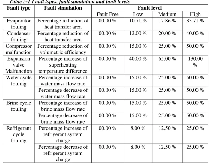
water and brine cycles, the simulation was performed by reducing or increasing the mass flow rate of the secondary fluids. For the refrigerant cycle, the simulation was done by decreasing or increasing refrigerant charge in the system. For each fault, the simulation was done by propagating the faults gradually on eleven steps between the nominal condition and extreme faulty conditions. Along the eleven steps, three main levels for each fault are introduced as low, medium and high faulty conditions in addition to the nominal operation condition (see Table 5.1).
Table 5-1 Fault types, fault simulation and fault levels
Fault type Fault simulation Fault level
Fault Free Low Medium High Evaporator
fouling
Percentage reduction of heat transfer area
00.00 % 10.71 % 17.86 % 35.71 %
Condenser fouling
Percentage reduction of heat transfer area
00.00 % 12.00 % 20.00 % 40.00 % Compressor malfunction Percentage reduction of volumetric efficiency 00.00 % 15.00 % 25.00 % 50.00 % Expansion valve Malfunction Percentage increase of superheating temperature difference 00.00 % 40.00 % 65.00 % 130.00 % Water cycle fouling Percentage increase of water mass flow rate
00.00 % 15.00 % 25.00 % 50.00 %
Percentage decrease of water mass flow rate
00.00 % 15.00 % 25.00 % 50.00 %
Brine cycle fouling
Percentage increase of brine mass flow rate
00.00 % 15.00 % 25.00 % 50.00 %
Percentage decrease of brine mass flow rate
00.00 % 15.00 % 25.00 % 50.00 % Refrigerant cycle fouling Percentage increase of refrigerant system charge 00.00 % 8.00 % 12.50 % 25.00 % Percentage decrease of refrigerant system charge 00.00 % 8.00 % 12.50 % 25.00 %
5.2 Fault Trend Analysis of Physical Parameters
In faults trend analysis, the aim here to identify physical feature that are easy to measure and yet describe heat pump unit performance and can capture the behavior of faults. The physical variables considered are temperatures points and compressor power input since temperature sensors and power input measurements are easy to obtain. thus making FDD more convenient and feasible to implement. The variables considered are 𝜟𝑻𝒆𝒗𝒂𝒑, 𝜟𝑻𝒔𝒖𝒑, 𝑻𝒅𝒊𝒔, 𝜟𝑻𝒔𝒖𝒃, 𝜟𝑻𝒘, 𝜟𝑻𝒃, 𝜟𝑻𝒄𝒐𝒏𝒅 and 𝑬𝒄𝒐𝒎𝒑 for fault trend analysis. After trend analysis is conducted, each one of the variables
mentioned above reacted to each fault by increasing, decreasing or stayed the same compared to the nominal conditions. In Table 5.2, the trend analysis results are shown as (↑↑) if the variable experienced a significant increase, (↑) if the variable experienced a moderate increase, (↓↓) if the
20
variable experienced a significant decrease, (↓) if the variable experienced a moderate decrease or (=) if the variable experienced a relatively slight increase or decrease or no change. The results of the trend analysis are shown in Table 5.2.
Table 5-2 Faulty characteristics of the heat pump parameters
Fault type 𝜟𝑻𝒄𝒐𝒏𝒅 𝜟𝑻𝒃 𝜟𝑻𝒘 𝜟𝑻𝒔𝒖𝒃 𝜟𝑻𝒔𝒖𝒑 𝜟𝑻𝒆𝒗𝒂𝒑 𝑻𝒅𝒊𝒔 𝑬𝒄𝒐𝒎𝒑 Evaporator fouling (=) (=) (=) (=) (=) (↓) (=) (=) Condenser fouling (↑↑) (=) (=) (↑↑) (=) (=) (↑↑) (=) Compressor vol. eff (↓) (↓) (↓) (↓) (=) (=) (↓) (↓↓) Exp. valve Malfunction (=) (=) (=) (↑) (↑↑) (↓↓) (↑↑) (=) Water under flow (↑) (=) (↑↑) (↑) (=) (=) (↑↑) (=) Water over flow (↓) (=) (↓) (↓) (=) (=) (↓) (=) Brine under flow (=) (↑↑) (=) (=) (=) (↓↓) (=) (=) Brine over flow (=) (=)(↓ at 50% or more) (=) (=) (=) (↑) (=) (=) Refrigerant leakage (=) (↓ at 25% or more) (=) (=) (↓↓) (=) (=) (=) (=) Refrigerant overcharge (↑) (=) (=) (↑↑) (=) (=) (↑) (=)
6 Sensitivity Ratio Method
The first approach used in this work for FDD modelling is the sensitivity ratio concept. This concept was previously used by (Chen. and Braun., 2000) to develop FDD model for air conditioners (air to air heat pumps). In this work this procedure is carried out to develop FDD model for brine to water ground source heat pumps using heat pump model developed in chapter 4.
The basic principle of the sensitivity ratio method is to find a pair of parameters for each fault in which one of them is significantly sensitive to that fault were the other is not sensitive to it. The fault sensitivity ratio (𝐹𝑅𝑓𝑎𝑢𝑙𝑡) is calculated as shown in Eq. [27].
𝐹𝑅𝑓𝑎𝑢𝑙𝑡 =𝑃𝑅𝑓𝑎𝑢𝑙𝑡,𝑖𝑛𝑠𝑒𝑛 𝑃𝑅𝑓𝑎𝑢𝑙𝑡,𝑠𝑒𝑛
21
Where 𝑃𝑅𝑓𝑎𝑢𝑙𝑡,𝑖𝑛𝑠𝑒𝑛 and 𝑃𝑅𝑓𝑎𝑢𝑙𝑡,𝑠𝑒𝑛 are insensitive and sensitive parameters residuals and they
are calculated as shown in Eq. [28].
𝑃𝑅𝑃𝐼 = |𝑃𝐼𝑎𝑐𝑡𝑢𝑎𝑙− 𝑃𝐼𝑖𝑑𝑒𝑎𝑙| [28]
Where 𝑃𝐼𝑖𝑑𝑒𝑎𝑙 are the value of the parameter when operating in fault free condition giving by the heat pump model and 𝑃𝐼𝑎𝑐𝑡𝑢𝑎𝑙is the measured value of that parameter. When a fault occurs, the insensitive parameter residual will equal nearly zero, where the sensitive parameter residual will increase. This lead to the value of 𝐹𝑅𝑓𝑎𝑢𝑙𝑡 to decrease below 1. If the value of 𝐹𝑅𝑓𝑎𝑢𝑙𝑡 is >= 1, this means that the corresponding fault is eliminated from the fault diagnosis process.
6.1 Physical Performance Indicators
For selecting relevant performance indicators and their tolerances, the absolute error value of each 𝑃𝐼 between the Matlab model and experiment data is calculated for each operation condition as shown in Table 6.1. The results showed that model predicts all parameter with sufficient accuracy except for 𝑻𝒅𝒊𝒔 which has been excluded from the FDD modeling.
Table 6-1 Absolute value of error between Matlab model and experiment data
𝑻𝒃,𝒊𝒏 𝑻𝒘,𝒊𝒏 𝜟𝑻𝒄𝒐𝒏𝒅 𝜟𝑻𝒆𝒗𝒂𝒑 𝜟𝑻𝒔𝒖𝒃 𝜟𝑻𝒔𝒖𝒑 𝜟𝑻𝒅𝒊𝒔 𝜟𝑻𝒃 𝜟𝑻𝒘 𝜟𝑬𝒄𝒐𝒎𝒑 -5 30 0.40 0.57 0.10 0.01 4.07 0.26 0.08 0.09 0 30 0.42 0.23 0.29 0.10 1.91 0.17 0.65 0.06 5 30 0.83 0.30 0.29 0.10 3.80 0.22 0.56 0.05 -5 40 0.11 0.62 0.05 0.01 4.86 0.31 0.46 0.01 0 40 0.80 0.38 0.19 0.18 5.62 0.20 0.27 0.01 5 40 0.49 0.32 0.40 0.08 3.63 0.17 0.24 0.02 -5 50 1.38 0.57 0.30 0.05 7.95 0.31 0.57 0.04 0 50 1.44 0.26 0.38 0.09 6.89 0.15 0.56 0.10 5 50 1.36 0.21 0.70 0.05 5.25 0.08 0.41 0.08
In this method, tolerances for each of the performance indicator residual are suggested to act as a minimum values of noise filters in measurements and to compensate for heat pump model errors. When the value of the residual is less than the tolerance, the parameter residual value is re-set to equal 0.1. These tolerance values can be adjusted to increase or decrease the sensitivity of the FDD model. The higher the tolerance value the less sensitive the FDD model and vice versa. For the FDD to work properly, calibrating parameters residuals’ tolerances are essential. For this thesis, and after analyzing the fault patterns operating in all nine operation conditions, a set of tolerance values is suggested in Table 6.2.
22
Table 6-2 Suggested tolerances for the parameters' residuals for each operation condition
Parameter residual
Tolerances values for each operation condition
W30B-5 W30B0 W30B5 W40B-5 W40B0 W40B5 W50B-5 W50B0 W50B5 𝑷𝑹𝜟𝑻𝒄𝒐𝒏𝒅 2.5 2.1 2.3 2.3 2.5 2.5 2.5 2.5 2.5 𝑷𝑹𝜟𝑻𝒆𝒗𝒂𝒑 0.8 0.8 0.8 0.8 0.83 0.8 0.77 0.94 0.75 𝑷𝑹𝜟𝑻𝒃 0.8 0.8 0.8 0.8 0.8 1.3 0.8 0.8 0.8 𝑷𝑹𝜟𝑻𝒘 1.3 1.3 1.3 1.3 1.3 1.3 1.8 2.9 2.7 𝑷𝑹𝜟𝑻𝒔𝒖𝒃 2.5 2 2 2.7 2.7 1.8 2.7 2 2 𝑷𝑹𝜟𝑻𝒔𝒖𝒑 2 2 1.8 1.8 1.8 0.8 1.8 1.5 1.2 𝑷𝑹𝑬 0.5 0.5 0.5 0.9 0.43 0.43 0.65 1 0.7
Based on the fault trend analysis (see Table 5.2), a pair of a sensitive and insensitive parameters is selected to calculate fault ratio for each fault as shown in Table 6.3.
Table 6-3 The sensitive and insensitive parameters and for each fault
Fault Sensitive parameter Insensitive parameter
Expansion valve malfunction 𝜟𝑻𝒔𝒖𝒑 𝜟𝑻𝒄𝒐𝒏𝒅
Water pump malfunction 𝜟𝑻𝒘 𝜟𝑻𝒆𝒗𝒂𝒑
Brine pump malfunction 𝜟𝑻𝒃 𝜟𝑻𝒄𝒐𝒏𝒅
Compressor malfunction 𝑬𝒄𝒐𝒎𝒑 𝜟𝑻𝒔𝒖𝒑
Evaporator fouling 𝜟𝑻𝒆𝒗𝒂𝒑 𝜟𝑻𝒄𝒐𝒏𝒅
Refrigerant charge 𝜟𝑻𝒔𝒖𝒃 𝜟𝑻𝒆𝒗𝒂𝒑
Condenser fouling 𝜟𝑻𝒄𝒐𝒏𝒅 𝜟𝑻𝒆𝒗𝒂𝒑
6.2 Fault Detection and Diagnosis Model Algorithm
When a fault develops in the system, at least one of the parameters’ residuals will exceed the tolerance value which will leads to the fault ratio of that fault to drop below 1. When 𝐹𝑅𝑓𝑎𝑢𝑙𝑡>1 the FDD model will detect a fault and a warning message will appear with the corresponding fault. The proposed algorithm is shown in Figure 6.1. The algorithm was tested using faulty data obtained from simulation using IMST-ART. A graphical user interface (GUI) is built for the model to facilitate using it as shown in Figure 6.2. The GUI need the ten parameters (nine temperature points and electric power) input, then after clicking Run, the model uses the heat pump model developed earlier to calculated the fault free conditions to be used as a reference. Then, the FDD model perform FDD algorithm (Figure 6.1) and display a message in System Diagnosis box containing the system diagnosis at that operation condition.
23
24
Figure 6-2 Graphical user interface for sensitivity ratio method based FDD model
6.3 Fault Detection and Diagnosis Model Results
For testing the FDD model, a set of data for fault free and faulty conditions (see table 5.1) is simulated for each operation condition (see table 4.1) is used. Using the algorithm shown in Figure 6.1, the FDD model were able to differentiate between all the faults successfully with the exception of the condenser blockage and refrigerant overcharge. When either condenser blockage or refrigerant overcharge fault propagate, they have similar symptoms that appear on the performance indicators (temperatures) behavior. Therefore, both condenser blockage and refrigerant overcharge are grouped in the diagnosis.
The sensitivity ratio method aims to identify the minimum fault level that can be detected for each fault during different operation conditions. Therefore, it is not able to identify the intensity of a fault when diagnosed. With using the suggested tolerance in Table 6.2, the FDD model were able to successfully detect and diagnose most fault for all operation conditions tested (see Table 4.1) within low and medium level of intensity with the exception of evaporator blockage and brine overflow. For both, Evaporator blockage and brine overflow the FDD model were able to detect and diagnose the fault only at extreme level conditions as shown in Figure 6.3. In Figure 6.3, fault levels equal to 4, 7 and 11 represent low, medium and high fault intensity respectively. (See Appendix 1 for result the operation conditions).
25
Figure 6-3 Fault type and level detected using sensitivity ratio method for operation conditions W30B0, W40B0 and W50B0
7 Principle Component Analysis Method
Principle component analysis (PCA) approach has been widely used in pattern recognition, performance monitoring, process control and fault detection and diagnosis in industrial process (Smith, 2002), (Shlens, 2003). It has been used in a wide range of application, from component level such as electrical machines (Ramahaleomiarantsoa et al., 2012), and mechanical components such as chillers/heaters (Chen and Lan, 2009), to large scale nuclear power plant (Ke, 2005). PCA approach is a mathematical technique that is used for dimensionality reduction of a multivariable system. PCA is usually used to transform a multivariable space into a new subspace with minimum amount of dimensions that preserve maximum variance of the original data. The original variables of the system are then linearly correlated to calculate a new set of variables known as principle components (PCs) whereas each PC value is a result of a linear correlation between all the original variables. The number of the PCs calculated is equal to the number of the original variable but arranged in descending order based on the variance of the original data along its axis. All the PCs are orthogonal to each other. This means that each PC captures along its axis data variance that is not captured by the other PCs. This allow us to reduce the number dimensions of the original data with preserving almost all the original data information (the more PCs we use the more data information we preserve). The benefit of this procedure is that it allows us to identify what is the minimum amount of PCs we need to choose to maintain maximum amount of original data information, thus we are able to minimize the system dimensions. For example, reducing the dimensionality of the data into two or three dimensions allows us to graphically visualize it thus makes it more convenient to recognize certain behaviors or patterns in the data.
0 1 2 3 4 5 6 7 8 9 10 11 Co n d . Fo u lin g| R ef. o ve rch arg e Eva p . F o u lin g W . u n d erfl o w W . o ve rf lo w R ef. u n d e rc h arg e B. u n d erfl o w B. o ve rf lo w E. v al ve Co m p re ss o r Fau lt Le vel W30B0 W40B0 W50B0
26
7.1 Principle Component Analysis Procedure
To perform PCA, Matlab function pca was used (Mathworks, 2015c). The PCA process is carried out in six main steps (see Appendix 3 for full X, V and D matrices used in the PCA procedure):
1) Obtaining training data from the original variables. In this step the fault free and
faulty data of the heat pump (simulated as describe in chapter 5) are used as the original data system. The original variables (dimensions) used are nine temperature measurements in addition to compressor electrical power input across the heat pump unit (𝑻𝟏, 𝑻𝟐, 𝑻𝟑, 𝑻𝒄𝒐𝒏𝒅, 𝑻𝟒, 𝑻𝟓, 𝑻𝟔, 𝑻𝟕, 𝑻𝟖, 𝑬𝒄𝒐𝒎𝒑). This data is represented as matrix
𝑿𝒏×𝒎, where m is number of columns and n is the number of rows. Each column
represents an original variable, whereas each row represents a sample data point of each variable (see the data matrix example in Figure 7.1).
Figure 7-1 Original data matrix
2) Mean normalizing of the original data matrix. This is done by subtracting the mean
of each variable (column) from each data point of that variable where 𝑿𝒎𝟏×𝒎 is a matrix that includes the mean values of each column in 𝑿𝒏×𝒎. This produces a new matrix 𝑿𝒏𝒐𝒓𝒎𝒂𝒍𝒊𝒛𝒆𝒅𝒏×𝒎 where each element in 𝑿𝒏×𝒎 is replaced by the mean of that variable (column) subtracted from that element. This means that each column (dimension) of the normalized matrix has a mean have of zero. This is done to facilitate the next step.
3) Finding the covariance matrix
Ʃ
of 𝑿𝒏𝒐𝒓𝒎𝒂𝒍𝒊𝒛𝒆𝒅𝒏×𝒎. Each covariance value in the covariance matrix represents the correlation between two variables in 𝑿𝒏𝒐𝒓𝒎𝒂𝒍𝒊𝒛𝒆𝒅𝒏×𝒎.A positive, negative or zero covariance value means that they are directly proportional, indirectly proportional or not correlated respectively. The covariance matrix is calculated using Eq. [29].
Ʃ = 1 𝑛 − 1∑(𝒙𝒊− 𝒙𝒎𝒆𝒂𝒏) 𝑛 𝑖=1 (𝒙𝒊− 𝒙𝒎𝒆𝒂𝒏)𝑻 [29]
Since the mean values of the normalized matrix is equal to zero, the formula can be rewritten as shown in Eq. [30]
Ʃ = 1 𝑛 − 1∑ 𝒙𝒊 𝑛 𝑖=1 𝒙𝒊𝑻 = 1 𝑛 − 1 𝑿𝒏𝒐𝒓𝒎𝒂𝒍𝒊𝒛𝒆𝒅 𝑻𝑿 𝒏𝒐𝒓𝒎𝒂𝒍𝒊𝒛𝒆𝒅 [30]
The result covariance matrix will be square symmetrical matrix
Ʃ
𝒎×𝒎 where the diagonal elements equal the variance of each column (dimension) in 𝑿𝒏𝒐𝒓𝒎𝒂𝒍𝒊𝒛𝒆𝒅.27
4) Finding the eigenvectors and eigenvalues of covariance matrix
Ʃ
𝒎×𝒎. The eigenvectors are calculated to identify the directions of the PCs. Each eigenvector represents the direction of one PC. In the other hand, the eigenvalues determine which eigenvector has the maximum variance along its axis, thus representing most of the system information. The higher the eigenvalue more variance the corresponding eigenvector has along its axis. Matlab function 𝒆𝒊𝒈 is used to find the eigenvectors (Mathworks, 2015a). This Matlab function returns vector matrix 𝐕𝒎×𝒎 and diagonalmatrix 𝐃𝒎×𝒎 that include the eigenvectors and eigenvalues respectively (see eigenvectors and eigenvalues matrix example in Figure 7.2).
Figure 7-2 Eigenvectors and eigenvalues
5) Choosing the number of dimensions 𝒌 where 𝒌 < 𝒎. In the previous step, all
eigenvectors obtained has a unit length. This means that by comparing the eigenvalues in terms percentages of summation of all eigenvalues (diagonal elements of 𝐃𝒎×𝒎),
the minimum eigenvectors (dimensions) can be identified while preserving most of the original data information. This is done by using Eq. [31]
𝑽𝒆𝒙𝒑,𝒋 = 𝒅𝒋 ∑𝑚 𝒅𝒊
𝑖=1
[31]
Where (𝑽𝒆𝒙𝒑) is the ratio of one eigenvalue with respect to the summation of all eigenvalues. After calculating (𝑽𝒆𝒙𝒑), usually the first few eigenvectors would represent almost all information (variance) of the original data.
6) Projecting the original data into the new selected dimensions. After choosing the
new number 𝒌 of eigenvectors (dimensions), the original data is projected into the new subspace by multiplying the original data matrix by the chosen eigenvectors as shown Eq. [32]
𝑨𝒏×𝒌 = 𝑿𝒏×𝒎 𝑽𝒎×𝒌 [32]
Where 𝑨𝒏×𝒌 is the projection matrix of the original data into dimensionally reduced subspace with 𝒌 dimensions (PCs).
28
Figure 7-3 Principle components analysis algorithm
7.2 Principle Component Analysis Results
The training data used for PCA included fault free and faulty data of the heat pump (simulated as describe in chapter 5). The original data matrix 𝑿𝒏×𝟏𝟎 (dimensions) used are nine temperature measurements in addition to compressor electrical power input across the heat pump unit (𝑻𝟏, 𝑻𝟐,
𝑻𝟑, 𝑻𝒄𝒐𝒏𝒅, 𝑻𝟒, 𝑻𝟓, 𝑻𝟔, 𝑻𝟕, 𝑻𝟖, 𝑬𝒄𝒐𝒎𝒑). After reforming PCA, ten eigenvectors 𝑽𝟏𝟎×𝟏𝟎 and eigenvalues 𝑫𝟏𝟎×𝟏𝟎 are found. The result of eigenvalues for each eigenvector is shown in Figure
7.4. The eigenvalues of the first, second and third eigenvectors are relatively high compared to the rest of the eigenvectors. This mean that they preserve most of the information about the system.