Published under the CC-BY4.0 license Open reviews and editorial process: Yes
Preregistration: No All supplementary files can be accessed at the OSF project page: https://doi.org/10.17605/OSF.IO/HXK2U
Graph Construction: An Empirical Investigation on Setting
the Range of the Y-Axis
Jessica K. Witt
Colorado State University
Graphs are an effective and compelling way to present scientific results. With few rigid guidelines, researchers have many degrees-of-freedom regarding graph construction. One such choice is the range of the y-axis. A range set just beyond the data will bias readers to see all effects as big. Conversely, a range set to the full range of options will bias readers to see all effects as small. Researchers should maximize congruence be-tween visual size of an effect and the actual size of the effect. In the experiments psented here, participants viewed graphs with the y-axis set to the minimum range re-quired for all the data to be visible, the full range from 0 to 100, and a range of approxi-mately 1.5 standard deviations. The results showed that participants’ sensitivity to the effect depicted in the graph was better when the y-axis range was between one to two standard deviations than with either the minimum range or the full range. In addition, bias was also smaller with the standardized axis range than the minimum or full axis ranges. To achieve congruency in scientific fields for which effects are standardized, the y-axis range should be no less than 1 standard deviations, and aim to be at least 1.5 stand-ard deviations.
Keywords: Graph Design, Effect size, Sensitivity, Bias
One way to lie with statistics is to set the range of the y-axis to form a misleading impression of the data. A range set too narrow will exaggerate a small effect and can even make a non-significant trend appear to be a substantial effect (Pandey, Rall, Sat-terthwaite, Nov, & Bertini, 2015). Yet the default set-ting of many statistical and graphing software pack-ages automatically sets the range as narrow as the data will allow. The problem of creating misleading graphs persists even when the full range is shown instead. As shown in the studies reported below, a
range set too wide also creates a misleading impres-sion of the data by making effects seem smaller than they are. Here, I argue that for scientific fields that use standardized effect sizes and adopt Cohen’s convention that an effect of d = 0.8 is big, the range of the y-axis should be approximately 1.5 standard deviations (SDs).
How should the y-axis range of a graph be deter-mined? Graph construction should account for the visual experience of the people reading the graphs (Cleveland & McGill, 1985; Kosslyn, 1994; Tufte, 2001) and the strong link between perception and cogni-tion (Barsalou, 1999; Glenberg, Witt, & Metcalfe, 2013). When the visual size of the effect aligns with the actual size of the effect, the person reading the graph does not have to exert mental effort to decode effect size from the graph. Instead, the size of the effect is processed automatically. This increases graph fluency by making it easier to understand
Jessica K. Witt, Department of Psychology, Colorado State University.
Data, scripts, and supplementary materials available at osf.io/hw2ac.
Address correspondence to JKW, Department of Psy-chology, Colorado State University, Fort Collins, CO 80523, USA. Email: Jessica.Witt@colostate.edu
Table 1. Overview of the five experiments.
Experiment N Effect sizes Graph Type Standardized condition1
1 9 0.1, 0.3, 0.5, 0.8 Bar graph 2 SDs
2 14 0.1, 0.3, 0.5, 0.8 Bar graph 1.4 SDs
3 13 0, 0.3, 0.5, 0.8 Bar graph with error bars 1.2 SDs
4 20 0, 0.3, 0.5, 0.8 Line graph 1.4 SDs
5 15 0, 0.3, 0.5, 0.8 Line graph 1 SD
Notes. 1This refers to the range depicted in the standardized condition, so a range of 1.4 SDs is when the
graph was centered on the grand mean and extended 0.7 SDs in either direction.
that an effect is big when it looks big and an effect is small when it looks small.
To increase graph fluency, the range of the y-axis should be selected to maximize compatibility be-tween visual size and actual effect size (Kosslyn, 1994; Pandey et al., 2015; Tufte, 2001). However, the current literature fails to provide clear guidelines on how to achieve this compatibility. For example, some recommend displaying only the relevant range so that the axis goes from just below the lowest data point to just above the highest data point (Kosslyn, 1994). This would not achieve the recommended compatibility because small effects would look big. Others assert that the y-axis should always start from 0, particularly for bar graphs (Few, 2012; Pan-dey et al., 2015; Wong, 2010). This too could fail to achieve compatibility by making effects look too small.
In the case of scientific fields for which effect size is standardized based on standard deviation, the range of the y-axis should be a function of the stand-ard deviation (SD). In behavioral sciences such as psychology and economics, for example, the mean effect size is approximately half a SD (Bosco, Aguinis, Singh, Field, & Pierce, 2015; Open Science Collabo-ration, 2015; Paterson, Harms, Steel, & Crede, 2016), and a standardized effect size of d = .8 is considered a big effect (Cohen, 1988). Consequently, an appro-priate range for the y-axis would be one to two SDs, which would be plotted as the group mean ± 0.75 SD (or ±0.5 – 1 SDs). With this range, big effects such as a Cohen’s d of .8 would look big and small effects of
d = .3 would look small. In other words, this range
would help achieve compatibility between the visual impression of the size of the effect and the actual size of the effect.
Empirical Studies
The effect of visual-conceptual size compatibility on graph fluency was empirically tested in 57 partic-ipants across 5 experiments (see Table 1). The par-ticipants were naïve college students, which serves as an appropriate sample given that scientific results should be accessible and comprehensible to this population and not just to experts in one’s field.
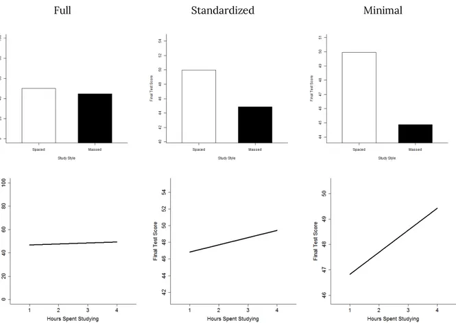
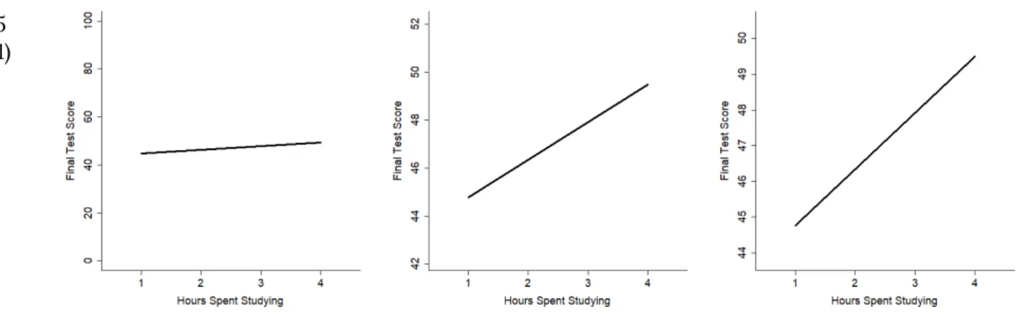
The stimuli were bar or line graphs that had been constructed from simulated data. Data were simu-lated from two (hypothetical) groups of participants by sampling from normal distributions in R (R Core Team, 2017). For one group, the data were drawn from a normal distribution with a mean of 50 and a standard deviation of 10 (as in a memory experiment with mean performance of 50% and SD of 10%). For the other group, the data were drawn from a normal distribution with a standard deviation of 10 and the mean at 49, 47, 45, or 42. These means correspond to effect sizes of d = 0.1, 0.3, 0.5, and 0.8, respec-tively. In Experiments 3-5, the mean of 49 (d = 0.1) was replaced with the mean of 50 (d = 0). In Exper-iments 2-5, the data were re-sampled if the attained effect size differed by more than 0.1 from the in-tended effect size. Data were simulated 10 times for each of the four effect sizes to create 40 sets of data for each Experiment. In Experiments 1-3, the means of the simulated data were displayed as a bar graph depicting two groups of participants who engaged in different study strategies (spaced versus massed; see Figure 1). In Experiments 4-5, the means were used to determine the end points of a line graph, and the x-axis was labeled as “hours spent studying”. For each set of data, three graphs were constructed that varied in the range of the y-axis. The full condition showed the full range from 0 to 100 on a hypothet-ical memory test. The minimal condition showed the smallest range necessary to see the data. The standardized condition was centered on the group
mean and extended by one to two SDs in either di-rection (the exact value differed across experiments, see Table 1 or the Appendix). Figure 1 shows several examples of graphs that served as stimuli. In Exper-iment 3, error bars were also included and explained to the participants. Within an experiment, the same set of 120 graphs (3 axis ranges x 4 effect sizes x 10 sets) were shown to the participants. Graphs were shown one at a time, order was randomized, and participants completed 4 blocks of 120 trials. In all experiments, the participants’ task was to indicate whether there was no effect, a small effect, a me-dium effect, or a big effect for each graph by press-ing 1, 2, 3 or 4 on the keyboard.
Graph fluency was measured using linear regres-sions rather than accuracy because regression coef-ficients have the advantage that they provide two separate measures. The slope provides an estimate of sensitivity to the magnitude of the effect depicted in the plot. A steeper slope indicates better sensitiv-ity to effect size than a shallower slope. The inter-cept provides an estimate of bias. Two graphs could lead to similar levels of sensitivity but different lev-els of bias. Separate linear regressions were calcu-lated for each participant for each y-axis range con-dition (full, standardized, and minimal).
Full Standardized Minimal
.
Figure 1. Sample stimuli in the experiments on bar graphs and on line graph. The bar graphs show final test score as a
function of whether study style was spaced or massed. The line graphs show final test score as a function of hours spent studying from 1 to 4. Within each experiment, the same data were plotted using the full range from 0-100, the standard-ized range (in this case, the group mean +/- 0.7 SD), or the minimal range necessary to see the data. In this example, a medium effect (Cohen’s d = 0.5) was simulated for the bar graphs (top row) and a small effect (Cohen’s d = 0.3) was simu-lated for the line graphs (bottom row). The participant’s task was to indicate whether there was no effect, a small effect, a medium effect, or a big effect.
In each regression, the dependent measure was response (on the scale of 1 to 4). The effect sizes were recoded to also be on a scale from 1 to 4 then centered by subtracting 2.5 so that perfect perfor-mance would produce a regression coefficient for the slope of 1 and an intercept of 2.5.
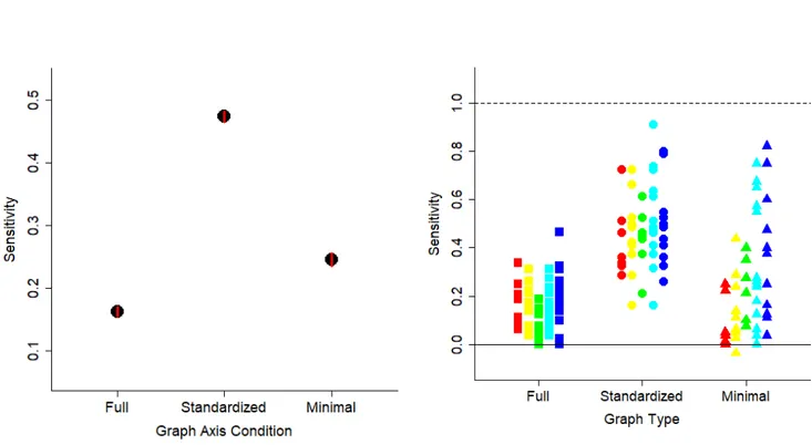
Figure 2 shows the mean slope coefficients across all 5 experiments. Sensitivity was best for the standardized graphs and worse for the full range graphs. Participants were better able to assess the size of the effect depicted in the graph for the stand-ardized graphs, than for the minimal or full graphs. Participants were also less biased when viewing the standardized graphs. Figure 3 shows the mean bias across all 5 experiments. Bias scores were calcu-lated as a percent bias based on the coefficients for
the intercept. A negative score indicates a bias to respond that effects were small, and a positive score indicates a bias to respond that the effects were big. For the full graphs, there was a large bias to respond that the effects were small. When looking at graphs with the full range, participants responded that al-most all effects (86%) were null or small. For the minimal graphs, there was a large bias to respond that the effects were substantial. When looking at graphs with the minimal range for Cohen’s d = 0.10 – 0.80, participants responded that the effect was big on 49% of the trials. In contrast, there was much less bias with the standardized graphs (see Supple-mental Materials).
Figure 2. Sensitivity is plotted as a function of graph axis condition for the three types of graphs across all 5 experiments.
Sensitivity was measured as the coefficient for the slope from regressions of actual effect size on estimated effect size. Only trials for which the graph depicted an effect size greater than d = 0.1 are included (see supplementary materials for all the data). A higher sensitivity score corresponds to better performance, and a coefficient of 1 corresponds to perfect performance. A coefficient of 0 indicates chance performance. In the left panel, mean sensitivity across all experiments is shown. Error bars are 1 SEM calculated within-subjects, and are approximately the same size as the symbols. The y-axis range is 3 SD. The right panel shows sensitivity for each participant for each experiment. The data are color-coded by experiment (e.g. red = Experiment 1, orange = Experiment 2) and are also laterally positioned from left to right within graph type category. Each point corresponds to one participant, and each participant has one symbol for each of the three graph types. The solid horizontal line at 0 shows the point of no sensitivity and the dashed horizontal line at 1 shows the point of perfect sensitivity.
Discussion
The visual impression of the size of an effect has a strong influence on the judged size of an effect. When the visual impression was compatible with the actual effect size, judgments of effect size were bet-ter calibrated and less biased compared with the typical default setting of showing the minimum range to display the data and the setting of showing the full potential range. Based on the current stud-ies, the recommendation is to center the y-axis on the grand mean and extend the range 0.75 SDs in ei-ther direction so that the range of the y-axis is 1.5 SDs.
The current studies show improved sensitivity to effect size and reduced bias in estimating effect size when the range of the y-axis was centered on the grand mean of the data and extended approximately 0.7 SDs in either direction. The various studies used slightly different extensions ranging from 0.5 SDs to 1 SD. There were not large detectable differences in sensitivity or bias depending on the exact range that
was used, so the precise value of the y-axis range might not be critical. Rather, the key feature is that the visual size aligns with the actual size of the ef-fect. The specific range to be used might vary as a function of the size of the error bars (the range should be large enough to encompass them), the size of the effect (the range would have to be ex-tended for particularly large effects, such as was done with the current results), if doing so would make the range include nonsensical numbers (such as negative numbers for performance), and to achieve a consistent scale across multiple graphs to enhance across-graph comparisons. Given that the exact range in terms of SD could vary from plot to plot, it could be useful to indicate the range in SD units in the figure caption. This indication would be particularly useful in cases for which researchers do not include error bars.
The current experiments explored graphs of stimulated data from between-subjects designs. The recommendations likely generalize to within-subject designs with the caveat that the y-axis
Figure 3. Bias (as a percentage) is plotted as a function of graph axis condition for the three types of graphs across all 5
experiments. A negative bias corresponds to responding that effects are smaller than they are, and a positive bias corre-sponds to responding that effects are bigger than their actual size. In the left panel, mean bias across all experiments is shown. Error bars are 1 SEM calculated within-subjects, and are approximately the same size as the symbols. The y-axis range is 4 SD. The right panel shows bias for each participant for each experiment. The data are color-coded by experi-ment (e.g. red = Experiexperi-ment 1, orange = Experiexperi-ment 2) and are also ordered from left to right within graph type category. Each point corresponds to one participant, and each participant has one symbol for each of the three graph types.
should be a function of the denominator used to cal-culate the within-subjects effect size. For example, the denominator for Cohen’s dz is the square root of the sum of the squares of the standard deviations minus the product of the standard deviations and the correlation between the two measures. Graphs plotting within-subjects data could be ± 0.75 times this denominator (or one of the other suggested measures for within-subjects effects sizes; e.g. Lakens, 2013). In cases for which there are both be-tween-subjects and within-subjects factors, the re-searchers will have to decide which denominator to use for the range depending on which effect they most want to emphasize.
It is debatable whether the recommendation of-fered here should be employed with bar graphs. Some have shown that graphs that start at a position other than 0 are deceptive (e.g., Pandey et al., 2015). The idea is that bar graphs should always start at 0 because the height of the bar signifies the value of the condition being represented. When the y-axis starts at a value greater than 0, the height of the bar corresponds to the difference between the condi-tion’s value and the starting point, rather than the condition’s value itself. Consider the following ex-ample: imagine that group A scored 70% on a memory test and group B scored 60%. On a plot for which the y-axis starts at 50%, group A’s score would appear twice as big as group B’s score, even though they only scored 10% higher. The issue at hand concerns the visual impression of the data. If the graph gives the impression that the differences are big, and that aligns with the size of the effect, the graph would be produce compatibility between vi-sion and true effect size. If, however, the impresvi-sion is that one group’s performance was twice as good as the other group’s performance, this would pro-duce a misleading impression of the data. The cur-rent experiments cannot speak to which impression was experienced because participants were asked to rate the size of the effect as being no effect, small, medium, or big, rather than quantifying the size of one bar relative to another. The specific task used here did not permit measuring the spontaneous im-pression given by the graphs. One option is for re-searchers to use alternative types of graphs to avoid the issue. Alternatives include point graphs and a newly-designed type of graph called a hat graph (Witt, 2019).
The recommendation to set the y-axis range to be 1.5 SDs does not generalize to fields for which the SD is unknown or irrelevant for interpreting effect size. For these fields, previous recommendations such as Tufte’s Lie Detector Ratio could be appro-priate (Tufte, 2001). But for scientific fields that rely on standard deviation to interpret effect size, this is the first empirically-based recommendation that provides clear guidelines for constructing graphs to communicate the magnitude of the effects.
Maximizing compatibility between visual size and conceptual size improved comprehension of the ef-fects shown in the graphs. The data presented in the graphs were exactly the same, yet participants were less biased and were more sensitive to the size of the depicted effect when the axis range was one to two SDs. Furthermore, emphasizing SD and effect size in graph construction could help shift researchers’ focus to effect size, rather than statistical signifi-cance. Indeed, effect size (as measured with Co-hen’s d) provides a better measure for discriminat-ing real effects from null effects than p values or Bayes factors (Witt, 2019). Such a shift could help guard against practices that have contributed to re-cent failures to replicate in various scientific fields (Camerer et al., 2016; Open Science Collaboration, 2015).
In his famous book on how to lie with statistics, Huff noted that as long as the y-axis is correctly la-beled, “nothing has been falsified – except the im-pression that it gives” (Huff, 1954, p. 62). The impres-sion matters. Researchers should select the range of the y-axis so that small effects look small and big effects look big (based on the field’s adopted con-ventions). A simple way to do this is to set the range to be 1.5 (or more) standard deviations of the de-pendent measure. That this improves graph com-prehension is both intuitive and is now supported by empirical evidence.
Open Science Practices
This article earned the Open Data and the Open Materials badge for making the data and materials
openly available. It has been verified that the analy-sis reproduced the results presented in the article. The entire editorial process, including the open re-views, are published in the online supplement.
Author contribution
Witt is solely responsible for this manuscript. The author read and approved the final manuscript.
Funding
This work was supported by grants from the Na-tional Science Foundation (1632222 and BCS-1348916).
Conflict of Interest Statement
The author declares there were no conflicts of interest.
References
Barsalou, L. W. (1999). Perceptions of perceptual symbols. Behavioral and Brain Sciences, 22, 577-660.
Belia, S., Fidler, F., Williams, J., & Cumming, G. (2005). Researchers misunderstand confidence intervals and standard error bars. Psychological
Methods, 10(4), 389-396. doi:
10.1037/1082-989X.10.4.389
Bosco, F. A., Aguinis, H., Singh, K., Field, J. G., & Pierce, C. A. (2015). Correlational effect size benchmarks. Journal of Applied Psychology,
100(2), 431-449. doi: 10.1037/a0038047
Camerer, C. F., Dreber, A., Forsell, E., Ho, T.-H., Huber, J., Johannesson, M., . . . Chan, T. (2016). Evaluating replicability of laboratory
experiments in economics. Science, 351(6280), 1433-1436.
Cleveland, W. S., & McGill, R. (1985). Graphical Perception and Graphical Methods for Analyzing Scientific Data. Science, 229(4716), 828-833. doi: 10.1126/science.229.4716.828
Cohen, J. (1988). Statistical Power Analyses for the
Behavioral Sciences. New York, NY: Routledge
Academic.
Collaboration, O. S. (2015). Estimating the reproducibility of psychological science.
Science, 349(6251), aac4716. doi:
10.1126/science.aac4716
Cumming, G., & Finch, S. (2005). Inference by eye: confidence intervals and how to read pictures of data. American Psychologist, 60(2), 170-180. doi: 10.1037/0003-066X.60.2.170
Few, S. (2012). Show Me the Numbers: Designing
Tables and Graphs to Enlighten (Second Edition
ed.). Burlingame, CA: Analytics Press. Glenberg, A. M., Witt, J. K., & Metcalfe, J. (2013).
From revolution to embodiment: 25 years of cognitive psychology. Perspectives on
Psychological Science, 8(5), 574-586.
Huff, D. (1954). How to Lie with Statistics. New York, NY: W. W. Norton & Company.
Kosslyn, S. M. (1994). Elements of Graph Design. New York: W. H. Freeman and Company. Lakens, D. (2013). Calculating and reporting effect
sizes to facilitate cumulative science: A practical primer for t-tests and ANOVAs.
Frontiers in Psychology, 4, 863. doi:
doi:10.3389/fpsyg.2013.00863
Morey, R. D., Rouder, J. N., & Jamil, T. (2014).
BayesFactor: Computation of Bayes factors for common designs (Version 0.9.8), from
http://CRAN.R-project.org/package=BayesFactor
Pandey, A. V., Rall, K., Satterthwaite, M. L., Nov, O., & Bertini, E. (2015). How Deceptive are
Deceptive Visualizations?: An Empirical Analysis of Common Distortion Techniques.
Paper presented at the Proceedings of the 33rd Annual ACM Conference on Human Factors in Computing Systems, Seoul, Republic of Korea. Paterson, T. A., Harms, P. D., Steel, P., & Crede, M.
(2016). An assessment of the magnitude of effect sizes: Evidence from 30 years of meta-analysis in management. Journal of Leadership
& Organizational Studies, 23(1), 66-81.
Revelle, W. (2018). psych: Procedures for
Psychological, Psychometric, and Personality Research. Retrieved from
R Core Team. (2017). R: A language and environment
for statistical computing. Retrieved from
https://www.r-project.org
Tufte, E. R. (2001). The Visual Display of
Quantitative Information (Second Edition ed.).
Cheshire, CT: Graphics Press.
Witt, J. K. (2019). Introducing hat graphs. Retrieved from psyarxiv.com/sg37q.
Witt, J. K. (2019). Insights into criteria for statistical significance from signal detection analysis.
Meta-Psychology, 3, MP.2018.871. doi:
10.15626/MP.2018.871
Wong, D. M. (2010). The Wall Street Journal Guide to
Information Graphics: The Dos & Don'ts of Presenting Data, Facts, and Figures. New York,
Appendix: Experimental Details
Experiment 1: Bar Graphs with Axis Range of 2 SD
Participants judged the size of effects depicted in bar graphs that were constructed with three axis range options.
Method
Participants. Nine students in an introductory
psychology course participated in exchange for course credit. In this and all subsequent experi-ments, the number of participants was maximized within a pre-determined time limit.
Stimuli and Apparatus. Graphs were
con-structed in R (R Core Team, 2017). For each graph, two means were generated. One mean was 50, and the other mean was 49, 47, 45, or 42. These equated to effect sizes of Cohen’s d = .1, .3, .5, and .8, respec-tively. To add some noise to each graph, each mean was drawn from a normal distribution centered on the desired mean with 1000 samples and a standard deviation of 10. The means were presented in bar graphs (see Figure A1). The left bar was white and labeled “Spaced” and the right bar was black and la-beled “Massed”. For each set of simulated data, three bar graphs were constructed that corre-sponded to the three y-axis range conditions. For
the full graphs, the y-axis range went from 0 to 100. For the minimal graphs, the y-axis went from the smallest data value minus 1 to the largest data value plus 1. For the standardized graphs, the mean of the two groups was calculated, and 1 SD (10) was added in either direction to set the y-axis range. This pro-cess of creating 3 graphs for each set of data was re-peated 10 times for each of the 4 effect sizes for a total of 120 graphs. Graphs were 500 pixels by 500 pixels and were shown on a 19” computer monitors with 1028 x 1024 resolution.
Procedure. After providing informed consent,
each participant was seated at a computer. They were given the following instructions: “You will see graphs showing the effect of study style on final test performance. There were two study styles. Massed is like cramming everything at once at just before the exam. Spaced refers to studying a little bit every day for weeks before the exam. The y-axis shows final test performance, with higher value meaning better performance.
Exp (SD
Range) Full Standardized Minimal
1 (2) 2 (1.4) 3 (1.2) 4 (1.4)
5 (1)
Figure A1. Sample stimuli for each of the 5 experiments. Each row corresponds to one experiment and
shows a single set of a data plotted in the three different ways (full, standardized, and minimal). In all cases, the data show a medium effect (Cohen’s d = 0.5). The number in parentheses under the experiment number indicates the range of the standardized condition.
For each graph, indicate if study style had 1. No effect, 2. A small effect, 3. A medium effect, 4. A big effect on final performance. Ready? Press ENTER”. A trial began with a fixation cross at the center of the screen for 500ms. The graph was then shown. Above the graph, text reminded participants of the four response options. The graph remained until participants made a response, at which point, the graph disappeared and a blank screen was shown for 500ms. Each block of trails consisted of the presen-tation of each of the 120 graphs (3 graph types x 4 depicted effect sizes x 10 repetitions). Order was randomized within block, and participants com-pleted 4 blocks for a total of 480 trials.
Results and Discussion
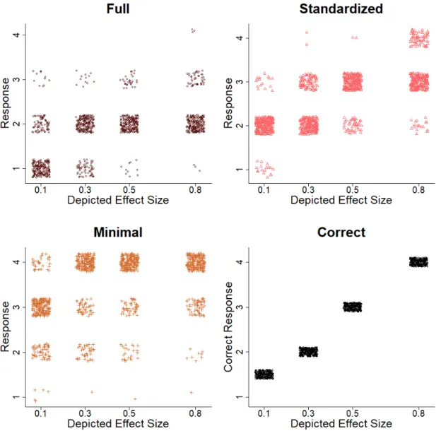
One participant only completed 431 trials, but their data were still included. The depicted effect size was recoded on a scale from 1 to 4 to be con-sistent with the scale of the response. The smallest effect size (d = .1) was coded as 1.5 to account for the idea that this effect is smaller than a small effect but bigger than no effect. In later experiments, these graphs were replaced with graphs for which there was no effect instead of d = .1.
For each participant for each of the 3 axis range conditions, the data were submitted to separate lin-ear regressions with estimated effect size as the de-pendent factor and actual effect size (recoded on a
scale from 1-4 then centered by subtracting 2.5) as the independent factor. The regressions produced two coefficients for each participant for each axis range condition. The slope indicates sensitivity to the size of the effect. A slope of 1 indicates perfect sensitivity. A slope less than 1 indicates attenuated sensitivity. The intercept indicates any bias to see effects as smaller or larger than their true size. One participant had slopes that were identified as outli-ers in the full and minimal conditions because they were greater than 1.5 times the interquartile range for each condition. This participant was excluded from the analysis (despite being the best performer in the group) because their data were not typical of the rest of the sample. Another participant had a slope less than 1.5 times the interquartile range in the full condition, and was also excluded for not be-ing typical of the rest of the sample.
The coefficients were analyzed using paired-samples t-tests to compare each graph condition to the others. Analyses were done in R (R Core Team, 2017). Bayes factors were calculated using the BayesFactor package in R with a medium prior (Mo-rey, Rouder, & Jamil, 2014). A Bayes factor greater than 3 indicates moderate evidence, and a Bayes factor greater than 10 indicates substantial evidence for the alternative hypothesis over the null hypoth-esis. Conversely, a Bayes factor less than .33 and less than .10 indicates moderate and substantial evi-dence for the null hypothesis over the alternative hypothesis. Effect sizes were calculated using the
recommendations of Lakens (2013), and 95% confi-dence intervals (CIs) on the effect size were calcu-lated using the cohen.d.ci function in the PSYCH package (Revelle, 2018).
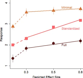
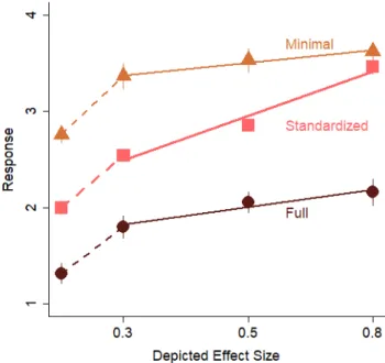
Figure A2. Mean response is plotted as a function
of depicted effect size and graph type for Experi-ment 1. Error bars are 1 SEM calculated within-subjects. Solid lines represent linear regressions for depicted effects d ≥ .3. Dashed lines represent lin-ear regressions for depicted effects less than d ≤ .3.
The standardized graphs produced significantly greater slopes than the full graphs, t(6) = 3.84, p = .009, dz = 1.45, 95% CIs [.33, 2.51], Bayes factor = 7.54 (see Figure A2). With the standardized y-axis range, participants were more sensitive to the differences in actual effect size (M = .47, SD = .11) compared with graphs that showed the full range from 0 to 100 (M = .30, SD = .07). Sensitivity was also better for the standardized graphs than the minimal graphs, t(6) = 3.61, p = .011, dz = 1.37, 95% CIs [.28, 2.40], Bayes fac-tor = 6.17. The minimal graphs (M = .28, SD = .04) produced sensitivity similar to the full graphs, p = .51, dz = .26, 95% CIs [-.50, 1.01], Bayes factor = 0.43.
These data show an advantage for the standard-ized graphs because participants were more sensi-tive to differences among magnitudes of the de-picted effect sizes with the standardized graphs than with the full or minimal graphs. However, the standardized graphs led to performance that was far
from perfect. The slope was .47, and perfect perfor-mance would have produced slopes of 1. Thus, even though the standardized graphs signify an improve-ment over the other two options, more work is still necessary to improve graph comprehension.
Another advantage for the standardized graphs can be seen with respect to bias. Bias scores were calculated as a percentage score of underestimation (negative values) and overestimation (positive val-ues). They were calculated as the participant’s co-efficient for the intercept minus the true intercept (2.5) divided by the true intercept. There were sig-nificant differences between the bias scores across all conditions, ps < .003. The bias scores for the full graphs was negative (M = -27%, SD = 10%) and sig-nificantly below 0, t(6) = -7.01, p < .001, dz = 2.64, 95% CIs [1.00, 4.27], Bayes factor = 82. The bias scores for the minimal graphs were positive (M = 36%, SD = 19%) and significantly above 0, t(6) = 4.91, p = .003, dz = 1.86, 95% CIs [.57, 3.10], Bayes factor = 19. In contrast, the bias scores for the standardized graphs were significantly less biased than in the other con-ditions (ps < .003), and were not significantly differ-ent from 0 (M = 1%, SD = 4%), t(6) = 0.47, p = .66, dz = .18, 95% CIs [-.58, .82], Bayes Factor = 0.39. With the full graphs, most effects looked like small effects. Indeed, 91% of the trials with the full graphs were labeled as showing no effect or a small effect. With the minimal graphs, 58% of the effects were labeled as big effects and 88% were labeled as medium or big. With the standardized graphs, small effects looked small and medium effects looked medium (see Figure A3). However, the big effects only looked medium. Thus, the experiment was replicated but with a smaller range in the standardized condition to determine if that would improve detection of big effects.
Experiment 2: Bar Graphs with Axis Range of 1.4 SD
Standardized graphs, for which the y-axis range is a function of the standard deviation, produced better sensitivity and less bias in participants who judged the size of the depicted effect compared with graphs that showed the full range and graphs that showed only the minimal range necessary to see the data. However, sensitivity with the standardized graphs was still below perfect performance. In this experiment, the range of the standardized graphs was decreased from 2 SDs to 1.4 SDs.
Method
Fourteen students in an introductory psychology course participated in exchange for course credit. Everything was the same in Experiment 1 except for the construction of the standardized graphs, for which the y-axis range went from the group mean minus 0.7 SD to the group mean plus 0.7 SD (see Fig-ure A1). Thus, the standardized range was 1.4 SD (in-stead of 2 SD as in Experiment 1). In addition, the
simulated data were evaluated to ensure that the outcomes were similar to the intended outcomes. The effect size of the simulated data were compared to the intended effect size, and if they differed by more than 0.1, the data were resampled until the dis-crepancy was less than 0.1. Participants completed 4 blocks of 120 trials, and order was randomized within block.
Figure A3. Response is plotted as a function of depicted effect size for the three types of axis range
condi-tions (full, minimal, and standardized) for Experiment 1. The bottom right panel shows the correct response. Response was entered as 1 (no effect), 2 (small effect), 3 (medium effect), and 4 (big effect). Each point cor-responds to one participant’s response on one trial. The data have been jittered along both axes to enable visibility.
Results and Discussion
The data were analyzed as before. Three partic-ipants had a slope that was deemed an outlier for being beyond at least 1.5 times the interquartile range for the full or minimal graphs.
The slope, which indicates sensitivity to the size of the effect in the graph, was greater for the stand-ardized graphs (M = .54, SD = .17) than the full graphs (M = .31, SD = .08), t(10) = 3.46, p = .006, dz = 1.04, 95% CIs [.28, 1.77], Bayes factor = 9.00 (see Figure A4). Sensitivity was also greater for the standardized graphs than the minimal graphs (M = .30, SD = .06), t(10) = 4.07, p = .002, dz = 1.23, 95% CIs [.42, 2.00], Bayes factor = 20. Replicating Experiment 1, the cur-rent data show that setting the range of the y-axis to be a function of the standard deviation, rather than the full range of options or the minimal range necessary to show the data, improved graph com-prehension. Recall, participants were not asked to indicate how big the effect looked but rather how big the effect was. Full and minimal graphs both produced misleading impressions of the data that severely attenuated sensitivity to effect size. Simply setting the range of the y-axis in relation to the standard deviation improved readers’ sensitivity to the data.
Figure A4. Mean response is plotted as a function of depicted effect size and graph type for Experi-ment 2. Error bars are 1 SEM calculated within-subjects. Solid lines represent linear regressions for depicted effects d ≥ .3. Dashed lines represent lin-ear regressions for depicted effects less than d ≤ .3.
Bias was again found for the full and minimal graphs but not the standardized graphs. For the full graphs, the bias was to underestimate effect size by 28% (SD = 9%), t(10) = -10.51, p < .001, dz = 3.17, 95% CIs [1.67, 4.64], Bayes factor > 100. Indeed, of all the trials with the full graphs, the effect was labeled as small or no effect on 90% of responses. The bias was of a similar magnitude but in the opposite direction for the minimal graphs, t(10) = 4.91, p < .001, dz = 1.48, 95% CIs [.59, 2.33], Bayes factor = 61. With the min-imal graphs, participants overestimated the size of the effects by 31% (SD = 21%). Over half of all effects with the minimal graphs were labeled big (53%), and 81% were labeled as medium or big. In contrast, the bias was much smaller (M = 6%, SD = 9%) for the standardized graphs, and only marginally signifi-cantly different from 0, t(10) = 2.13, p = .059, dz = .64, 95% CIs [-.02, 1.28], Bayes factor = 1.50. The bias with the standardized graphs was far less than the biases observed with the full and minimal graphs, ps < .001.
The evidence thus far is clear: graphs with a y-axis range that is a function of the standard devia-tion produces better sensitivity and less bias in par-ticipants when they are tasked with judging the size of an effect, compared with graphs that present the full range and with graphs that present only the minimal range necessary to view all of the data.
Experiment 3: Bar Graphs with Error Bars
The graphs in Experiments 1 and 2 did not contain error bars. As a result, the graphs did not contain enough information to know if an effect was null, small, medium, or big. This was a conscious decision given that introductory psychology students might not know how to interpret error bars. Yet, it is nec-essary to know if standardized graphs still produce an advantage even when there is enough infor-mation presented in the graphs to be able to accu-rately answer the question. In addition, the graphs
with the smallest effects in Experiments 1 and 2 had the awkward feature of being bigger than no effect but smaller than a “small” effect, so it was unclear whether the correct answer should be 1 or 2. This ambiguity was eliminated in the current experiment.
Method
Thirteen students in an introductory psychology course participated in exchange for course credit.
Graphs were constructed similarly as in Experi-ment 2 with the following exceptions. The four ef-fect sizes that were modeled were Cohen’s d = 0, .3, .5, and .8, which corresponds to no effect, a small ef-fect, a medium efef-fect, and a big efef-fect, respectively. The data were simulated as coming from two inde-pendent groups of 100 participants. The mean used to model the data for the hypothetical group that used the spaced studying strategy was always 50 (as in 50% accuracy on a memory test). The mean used to model the data for the hypothetical group that used the massed studying strategy was 50 minus 0, 3, 5, or 8 depending on the effect size being mod-eled. Using these means and a SD of 10, data were sampled from a normal distribution and summarized for the graphs. Error bars were calculated as 95% confidence intervals. In addition to the instructions given in Experiments 1 and 2, participants were also told the following: “Important! An effect is statisti-cally significant if p < .05. However, you can also as-sess statistical significance by looking at error bars. Error bars are lines that extend from the mean of each condition. The mean of each condition is shown by the top of the bar. If the error bar from one condition overlaps the mean from the other condition, the effect is NOT significant. If neither bar overlaps the mean of the other condition, then the effect is significant. The farther apart the error bars, the bigger the effect.” Note that this rule of thumb is overly simplified. There can be cases for which the error bars overlap but the effect is statis-tically significant at the p < .05 level (Cumming & Finch, 2005), but this level of nuance was not pre-sented to the participants.
For each set of simulated data, 3 graphs were constructed. For the full graphs, the y-axis range went from 0 to 100. For the standardized graphs, the y-axis range went from the grand mean minus 0.6 SD to the grand mean plus 0.6 SD. For the min-imal graphs, the bottom of the y-axis range was the
smallest combination of the mean minus the lower confidence interval minus 0.1, and the top of the range was the biggest combination of the mean plus the upper confidence interval plus 0.1. Participants completed 4 blocks of 120 randomized trials.
Results and Discussion
The data were analyzed as before. One partici-pant had a negative slope for the standardized graphs, and another participant had a high slope for the full graphs. Both were 1.5 times beyond the in-terquartile range and excluded from analyses.
Figure A5. Mean response is plotted as a function of depicted effect size and graph type for Experiment 3. Er-ror bars are 1 SEM calculated within-subjects. Solid lines represent linear regressions for depicted effects d ≥ .3. Dashed lines represent linear regressions for depicted ef-fects less than d ≤ .3.
The slopes were steeper, showing better sensi-tivity, for the standardized graphs (M = .62, SD = .19) compared with the full graphs (M = .24, SD = .09) and the minimal graphs (M = .55, SD = .20). The differ-ence in slopes between the standardized and full graphs was significant, t(10) = 7.76, p < .001, dz = 2.34, 95% CIs [1.16, 3.50], Bayes factor > 100. The differ-ence in slopes between the standardized versus minimal graphs was also significant, t(10) = 3.09, p = .011, dz = .93, 95% CIs [.20, 1.63], Bayes factor = 5.46. Even though all the information was the same across
the three graph conditions and even though this in-formation was sufficient for determining the size of each effect, participants were better able to deter-mine effect size when the range of the y-axis was a function of the standard deviation (see Figure A5).
The impression given by Figure A3 indicates that sensitivity was just as good if not better for the min-imal graphs than the standardized graphs when comparing no effect to a small effect (ds = 0 and .3), but sensitivity was better (steeper) for the standard-ized graphs when comparing across small, medium, and big effects (ds = .3, .5, and .8). This impression prompted an unplanned analysis. Linear regres-sions were again conducted for each participant for each graph condition. However, in one set of re-gressions, only effect sizes 0 and .3 were included. In another set of regressions, only effect sizes .3, .5, and .8 were included. Two additional participants were identified as outliers because the slopes for all three graphs in the latter analysis were 1.5 times be-yond the interquartile range, and were excluded from the remaining analyses.
With respect to determining whether or not an effect is present (by comparing slopes for graphs de-picting ds = 0 and .3), all three graph types led to similar performance (Standardized: M = .89, SD = .40; Full: M = .49, SD = .22; Minimal: M = 1.02, SD = .45). With all three types of graphs, participants were sensitive to whether or not there was an effect, as shown by coefficients for each graph type that were positive and significantly greater than 0, ps < .001. The standardized graph produced some benefit over the full graphs, t(8) = 2.82, p = .022, dz = .85, 95% CIs [.14, 1.53], Bayes factor = 3.76. The standardized graph was no better, and marginally worse, than the minimal graphs, t(8) = -1.82, p = .11, dz = .55, 95% CIs [-.10,1.17], Bayes factor = 1.03. It should be noted that a bias to see all effects as being bigger (as found with minimal graphs) would lead to a steeper slope when comparing just the graphs that depict a null effect and a small effect. Thus, it cannot be known whether sensitivity is better with the minimal graphs or if the bias caused by the minimal graphs leads to greater estimates of sensitivity.
With respect to determining the magnitude of an effect that is present (by comparing slopes for graphs depicting ds = .3, .5, and .8), the standardized graphs produced better sensitivity than the full or
minimal graphs (Standardized: M = .46, SD = .11; Full: M = .09, SD = .06; Minimal: M = .25, SD = .13), ps ≤ .001. The comparison between the standardized graphs to the full graphs resulted in a Bayes factor greater than 100, dz = 2.81, 95% CIs [1.45, 4.14]. The comparison between the standardize graphs to the minimal graphs resulted in a Bayes factor of 65, dz = 1.50, 95% CIs [.60, 2.35]. In each of the three graph types, participants showed some level of sensitivity to the magnitude of the effect, as shown by the co-efficients being significantly greater than 0, ps < .003.
In addition to better sensitivity with the stand-ardized graphs, the standstand-ardized graphs also pro-duced less bias compared with the other graphs, ps <= .001. For the full graphs, there was a 28% bias (SD = 12%) to underestimate effect size, which was sig-nificantly different from 0, t(10) = -7.82, p < .001, dz = 2.36, 95% CIs [1.17, 3.52], Bayes factor > 100. For the minimal graphs, there was a 14% bias (SD = 24%) to overestimate the size of the effect, which was marginally significantly from 0, t(10) = 2.03, p = .069, dz = .61, 95% CIs [-.05, 1.25], Bayes factor = 1.33. For the standardized effects, the bias was 7% (SD = 19%) and was not significantly different from 0, t(10) = 1.29, p = .227, dz = .39, 95% CIs [-.23, .99], Bayes fac-tor = .58.
In summary, even with error bars, graphs with the y-axis range set as a function of the standard de-viation produced better sensitivity and less bias compared with graphs that showed the full range and graphs that showed only the minimal range nec-essary to see the data.
Experiment 4: Line Graphs with Axis Range of 1.4 SD
The current experiment used line graphs as stim-uli instead of bar graphs to see if the previous rec-ommendations generalized to a different kind of graph.
Method
Twenty students in an introductory psychology course participated in exchange for course credit. Stimuli were graphs that were constructed by sim-ulating data from two groups, and connecting their means with a line to create an impression of data across four groups. The four effect sizes that were
modeled were Cohen’s d = 0, .3, .5, and .8, which cor-responds to no effect, a small effect, a medium ef-fect, and a big efef-fect, respectively. The y-axis range was full (0-100), minimal (smallest value minus 1 to largest value plus 1), or standardized (group mean minus 0.7 SD to the group mean plus 0.7 SD). Eve-rything else was the same as in the previous experi-ments, except the x-axis was labeled as hours spent studying on a range from 1-4.
Results and Discussion
The data are shown in Figure A6. The data were analyzed as before with three separate linear re-gressions for each participant for each graph type for each combination of all effect sizes, d = 0 and .3 only, and d = .3 - .8 only. One participant had slopes greater than 1.5 times the interquartile range for the full and minimal graphs, and 3 participants had slopes less than 1.5 times the interquartile range for the minimal graphs. All 4 were excluded.
For regressions on all effect sizes depicted in the graphs, the standardized graphs lead to greater slopes than the full graphs, t(15) = 7.16, p < .001, dz = 1.79, 95% CIs [.98, 2.59], Bayes factor > 100 (see Table A1). The standardized graphs did not lead to signifi-cantly different slopes than the minimal graphs when calculated across the entire range, t(15) = 0.18, p = .86, dz = .05, 95% CIs [-.45, .53], Bayes factor = .26. However, this is because the minimal graphs produced superior performance with respect to de-termining whether there was an effect or not but in-ferior performance when an effect was present and the magnitude had to be determined. For regres-sions comparing d = 0 to d = .3, the slopes for the minimal graphs were higher than for the standard-ized graphs, t(15) = -4.70, p < .001, dz = 1.17, 95% CIs [.52, 1.81], Bayes factor > 100. Again, recall that the bias generated by the minimal graphs to see effects as bigger would produce greater sensitivity scores even if participants were not necessarily more sen-sitive to the effect. Indeed, the slope coefficient is 1.29, which is greater than perfect accuracy of 1, which implies some bias. For regressions comparing ds > 0, the slopes for the standardized graphs were higher than for the minimal graphs, t(15) = 3.05, p = .008, dz = .76, 95% CIs [.19, 1.31], Bayes factor = 6.46. This suggests that the standardized graphs still pro-duced better outcomes than the full or minimal graphs.
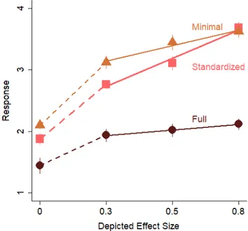
Figure A6. Mean response is plotted as a function of depicted effect size and graph type for Experi-ment 4. Error bars are 1 SEM calculated within-subjects. Solid lines represent linear regressions for depicted effects d ≥ .3. Dashed lines represent lin-ear regressions for depicted effects less than d ≤ .3.
Table A1.
Mean (and SD) coefficients for the slopes for each graph type for each analysis from Experiment 4.
Graph Type All data ds = .3-.8 ds = 0 - .3
Full .30 (.08) .15 (.08) .61 (.22) Standardized .61 (.15) .52 (.18) .86 (.32) Minimal .61 (.06) .31 (.25) 1.29 (.56)
Note. The slopes indicate the linear relationship between the size of the effect depicted and the estimate of the ef-fect size, both of which were coded on a scale from 1-4.
Regarding bias, similar results were found as in previous experiments. The bias was -26% (SD = 11%) with the full graphs, indicating a bias to underesti-mate the effects, t(15) = -9.52, p < .001, dz = 2.38, 95% CIs [1.39, 3.34], Bayes factor > 100. The bias was 19% (SD = 17%) with the minimal graphs, indicating a bias
to overestimate the size of the effects, t(15) = 4.36, p < .001, dz = 1.09, 95% CIs [.46, 1.70], Bayes factor = 64. With the standardized graphs, the bias was 2% (SD = 10%), which was not significantly different from 0, t(14) = 0.73, p = .48, dz = .18, 95% CIs [-.31, .67], Bayes factor = .32. With the line graphs, as with the bar graphs, the standardized axis range produced better sensitivity and less bias than the full axis range or the minimal axis range.
Experiment 5: Line Graphs with Axis Range of 1 SD
The current experiment replicated Experiment 4 using a smaller axis range for the standardized graphs.
Method
Fifteen students in an introductory psychology course participated in exchange for course credit. The stimuli were the same as in Experiment 4 except that for the standardized graphs, the range was the group mean ± 0.5 SD.
Results and Discussion
The data were analyzed as before with three sep-arate linear regressions for each participant for each graph type for each combination of all effect sizes, d = 0 and .3 only, and d = .3 - .8 only. One participant had a slope that was less than 1.5 times the inter-quartile range for the minimal graphs, and one had a slope greater than 1.5 times the interquartile range for the full graphs. Both were excluded. The mean slope coefficients for the remaining participants are shown in Table A2 and the data are shown in Figure A7.
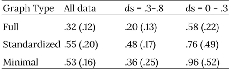
Table A2.
Mean (and SD) coefficients for the slopes for each graph type for each analysis from Experiment 5.
Graph Type All data ds = .3-.8 ds = 0 - .3
Full .32 (.12) .20 (.13) .58 (.22) Standardized .55 (.20) .48 (.17) .76 (.49) Minimal .53 (.16) .36 (.25) .96 (.52)
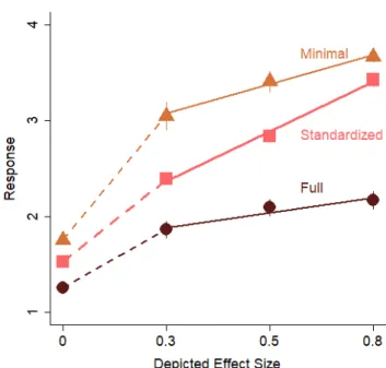
Figure A7. Mean response is plotted as a function of depicted effect size and graph type for Experi-ment 5. Error bars are 1 SEM calculated within-subjects. Solid lines represent linear regressions for depicted effects d ≥ .3. Dashed lines represent lin-ear regressions for depicted effects less than d ≤ .3.
The patterns match those found in Experiment 4. Participants were more sensitive to the size of the effect for the standardized graphs than for the full graphs when all trials were included, t(13) = 4.41, p < .001, dz = 1.22, 95% CIs [.48, 1.94], Bayes factor = 46, and when trials for which the effect size depicted was greater than 0, t(13) = 6.69, p < .001, dz = 1.86, 95% CIs [.93, 2.76], Bayes factor > 100, but not when only trials for which the effect size depicted was null or small, t(13) = 1.41, p = .19, dz = .39, 95% CIs [-.18, .95], Bayes factor = .62. Participants were more sen-sitive to the size of the effect for the standardized graphs than for the minimal graphs but only when the depicted effect in the graph was greater than 0, t(13) = 2.59, p = .023, dz = .72, 95% CIs [.09, 1.32], Bayes factor = 2.88. There was no difference in sen-sitivity across all effect sizes, p = .65, Bayes factor = .31, and the minimal graphs produced better sensi-tivity when only data from graphs depicting a null or small effect were included, t(13) = -3.11, p = .009, dz = .86, 95% CIs [.21, 1.49], Bayes factor = 6.27. As be-fore, the bias created by the minimal graphs could account for this apparent increase in sensitivity.
Regarding the bias, the full graphs produced a bias of -15% (SD = 17%), indicating a bias to underes-timate effect size, t(12) = -3.07, p = .010, dz = .85, 95% CIs [.20, 1.48], Bayes factor = 5.90. The minimal graphs produced a bias of 12%, (SD = 20%), which was marginally above 0, t(12) = 2.21, p = .047, dz = .61, 95% CIs [.01, 1.20], Bayes factor = 1.69. The stand-ardized graphs led to a small bias of 6% (SD = 14%), that was marginally close to 0, t(12) = 1.63, p =.13, dz = .45, 95% CIs [-.13, 1.01], Bayes factor = .80.
Across Experiment Comparisons
Sample size was not selected to achieve sufficient power to do analyses across experiments. To facili-tate preliminary exploration of the data, the coeffi-cients are reported in Tables S3, S4, and S5, and are plotted in Figure A8 and Figures 2 and 3 in the main
text. It may be interesting to note that sensitivity of the size of the effect was not notably better with er-ror bars than without erer-ror bars even though erer-ror bars are necessary to understand effect size. Alt-hough this may not be surprising given the partici-pants being introductory psychology student, the pattern is consistent with previous findings that many researchers do not know how to interpret er-ror bars (Belia, Fidler, Williams, & Cumming, 2005). In addition, the lack of noticeable differences in sen-sitivity between the experiments suggests that the use of a y-axis range that is approximately 1.5 SDs could help better report the results in cases for which researchers neglect to include error bars.
Table A3.
Mean slopes (and standard deviations) from regressions on all trials for each of the 5 experiments.
Graph Type Exp 1 Exp 2 Exp 3 Exp 4 Exp 5
Full .28 (.10) .31 (.08) .21 (.08) .30 (.08) .32 (.13) Standardized .46 (.13) .54 (.17) .58 (.17) .61 (.15) .55 (.20) Minimal .27 (.03) .30 (.06) .49 (.15) .61 (.06) .53 (.16)
Note. A slope of 1 indicates perfect performance and a slope of 0 indicates chance performance.
Table A4.
Mean slopes (and standard deviations) from regressions on trials for which Cohen’s d > 0.1 for each of the 5 experiments.
Graph Type Exp 1 Exp 2 Exp 3 Exp 4 Exp 5
Full .17 (.10) .18 (.10) .09 (.06) .15 (.08) .20 (.13) Standardized .42 (.16) .46 (.16) .46 (.11) .52 (.18) .48 (.17) Minimal .07 (.09) .13 (.14) .25 (.13) .31 (.25) .36 (.25)
Table A5.
Mean bias scores as a percentage (and standard deviations) for each of the 5 experiments.
Graph Type Exp 1 Exp 2 Exp 3 Exp 4 Exp 5
Full -27 (5) -28 (9) -25 (10) -26 (11) -15 (17) Standardized 1 (4) 6 (9) 14 (13) 2 (10) 6 (14) Minimal 36 (21) 31 (21) 23 (16) 19 (17) 12 (20)
Note. Bias scores were calculated as a percent bias based on intercepts from regressions on all trials including those for which Cohen’s d = 0.