1995:19 Non-destructive Assay of Spent BWR Fuel with High-resolution Gamma-ray Spectroscopy

-SKI Report 95: 19

Non-destructive Assay of Spent

BWR Fuel with High-resolution

Gamma-ray Spectroscopy

Ane Hakansson

Anders Backlin

May 1995

ISSN 1104-1374 ISRN SKI-R--95/19--SE

SK

i

SKI Report 95: 19

Non-destructive Assay of Spent

BWR Fuel with High-resolution

Gamma-ray Spectroscopy

Ane Hakansson

Anders Backlin

Department of Radiation Sciences, Uppsala University,

Box 535, S-751 21 UPPSALA

May 1995

This report concerns a study which has been conducted for the Swedish Nuclear

Power Inspectorate (SKI). The conclusions and viewpoints presented in the report

1995-03-01

Non-destructive assay of Spent BWR Fuel with

High-Resolution Gamma-ray Spectroscopy

Ane HAkansson and Anders Backlin

Department of Radiation Sciences, Uppsala University

Abstract

A method, based on high-resolution gamma-ray spectroscopy, has been developed for verification of burnup, cooling time, power history and, to some extent, the initial enrichment of spent BWR fuel. It is shown that, provided that the power history is known and corrected for, bumup and cooling time can be verified with accuracies within 3% and 60 days, respectively, for cooling times up to about 20 years. For cooling times up to about 50 years the corresponding accuracies are 3% and 1.5 years. It is also shown that the above parameters can be determined with no other information than the fuel type. In such cases the accuracies are 3.2% and 170 days, respectively (cooling time <20 years) and 6% and 2 years (cooling time <50 years).

I denna rapport beskrivs en metod baserad pa hogupplosande gammaspektroskopi att anvandas for verifiering av utbranningsgrad, avklingningstid och, i viss man, initial anrikning for BWR bransle. Forutsatt att korrektion for effekthistorik utfors kan utbrannmg och avklingningstid med den har beskrivna metoden bestammas inom 3% respektive 60 dagar for avk1ingningstider mindre an ca 20

At.

For avk1ingningstider upp till 50

At

uppskattas verifieringsnoggrannheten till ca 3% respektive 1.5

At.

I rapporten visas ocksa att ovanstaende parametrar kan bestammas utan annan kannedom om bransleelementen an bransletyp. Noggrannheten i bestiimningen av parametrama minskas i sadana fall till 3.2% respektive 170 dagar (avk1ingningstid < 20

At)

och 6% respektive 2

At

(avklingningstid

1 INTRODUCTION

2 THE HRGS METHOD FOR BWR FUEL.

2.1 Basic fuel parameters. 2.2 Principle of the experiment. 2.3 Determination of the burnup 2.4 Determination of the cooling time 2.5 The Power history.

2.6 The initial enrichment

2.7 Correction for fuel pin configuration

3 EXPERIMENTAL EQUIPMENT

3.1 The mechanical arrangement 3.2 The detector system

3.3 Software

3.4 Reference source

4 MEASUREMENTS

5 RESULTS

5.1 Procedure of evaluation and presentation

5.2 Determination of the calibration constants

Kx

and K

5.2.1 137CS

5.2.2 134CS and 154Eu

5.3 Simultaneous determination of BU and CT 5.3.1 134CS and 137es

5.3.2 15"Eu and 137es

5.4 Determination of CT from the ratio 154Euf34Cs

6 DISCUSSION

7 ACKNOWLEDGEMENTS

8 REFERENCES

3

3

3 4 6 7 7

10

10

11

11 12

14

17

17

18

18

20

20

21 23 24

26

26

28

29

29

1

Introduction

The need of experimental methods for verification or identification of spent nuclear fuel for safeguard purposes is generally recognised. Of immediate interest are methods to verify that nuclear power plants have been operated as stated by their operators and that the spent fuel with its contents of fissile material has not been manipulated during its transportation or storage. Later, at the end of the fuel cycle, the fuel will be pennanently encapsulated and placed in the final repository. Safeguard reasons will then demand a high degree of assurance that the nuclear material encapsulated is in accordance with the book-keeping.

Non-destructive assay of spent nuclear fuel can be made by measuring the radiation emitted, either neutrons or gamma-rays. High-Resolution Gamma-Ray Spectroscopy (HRGS) is a potentially useful method for verification and identification of spent fuel. It is based on measurements of the concentration of the fission products 137Cs, 134CS and 15"EU. Advantages with this method are: (i) Two or more isotopes with different gamma-ray energies are measured, which give information on different fuel parameters (see below). (H) The relationship between the concentration of 137 Cs and the burnup of the fuel is very nearly linear. (Hi) The measurement is passive, i. e. no external radiation source is needed. (iv) The primary data registered are spectroscopic in character, implying that the quality of the measurement can easily be checked by inspecting a computer screen. This may be used to identify and eliminate problems that may arise from disturbing electric fields or other malfunctions.

The HRGS method has been discussed earlier, see e. g. ref. 11 - 4/. It has been studied and further developed in Sweden during several years in a co-operation between the Department of Radiation Sciences at Uppsala University and the Swedish Nuclear Power Inspectorate (SKI). In the present report we describe the equipment developed for the work, the methods for analysing the data and some results obtained. Parts of this work has been reported earlier, ref.

IS -

8/.

2

The HRGS method for BWR fuel.

2.1

Basic fuel parameters.

In spent nuclear fuel the concentration of fission products at a given moment depends on a number of quantities or circumstances, in the following called fuel parameters, which are characteristic for an individual fuel assembly. The most important fuel parameters in the present context are:

Burnup(BU) Cooling time (CT) Initial enrichment Power history Integrity

The parameters represent averages over the whole fuel assembly. The parameter "integrity" is introduced in order to account for the fact that assemblies sometimes have been reconstructed in such a way that the original rods have been replaced or, sometimes, removed.

Of the five parameters listed, BU and CT are by far the most important for the concentrations of the fission products. By measuring the gamma-ray intensities from two fission products, these two quantities can be determined to first order since the fission products all have different half-lives. The three remaining fuel parameters have less influence on the concentrations of the fission products. The power history has an observable influence on the intensities measured, implying that this parameter to some extent can be verified in the measurements. In practice this is done by using the operator declared values for the relevant parameters for calculating corrections to the values of BU and CT obtained in first order. If the measurements are accurate enough significant deviations

between the corrected experimental values of BU and

er

and the operator's declared values will then result if the actual power history deviates from the declared one.

The influence of the two remaining fuel parameters, the original enrichment and the integrity, have not been studied in detail here. Calculations with the code ORIGEN 2, ref. /9/, indicate that the yields of 134CS and lS~U depend somewhat on the initial enrichment. Our data suggest that this parameter

only has, a minor influence on the gamma-ray intensities measured here. We have accordingly attempted a simplified procedure of correction for the influence of this parameter as presented in section 2.6. A more detailed treatment is, however, required in order to conclude to what degree of accuracy the initial enrichment can be determined with the HRGS method

The present set of data defmitely indicate that the gamma-ray intensities are sensitive to the integrity of the fuel assemblies. It has however not been possible here to make a quantitative study of this effect

2.2

Principle of the experiment.

The concentration of 137CS depends almost linearly on BU. In a typical Swedish BWR fuel the

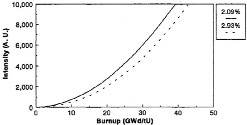
deviation from linearity for BU below 40 GWdltU is less than 0.2% as calculated with the code ORIGEN 2, ref. /9/. For 134CS and lS~U the relation between the concentration and BU is more

complex, see figs. 2.1 and 2.2.

1 4 0 , 0 0 0 , . - - - " " ' 7 - - - : - , , . - - - , 120,000

;r

100,000

$

so,ooo

~ ~ 60,000 oS .E 40,000 20,000 00 ₁₀ 2.09% 2.93% 20 30 40 50 Bumup (GWdltU)

Figure 2.1. The J34CS intensity as calculated with ORlGEN 2 for two different initial enrichment v. s. burnup. 10,000 8,000 ~

i

6,000 ~ '; c _4,000 oS .E 2,000 0 0 10 20 30 Bumup (GWd/tU) 40

~

L:J

50

Figure 2.2. Same as infig. 2.1 but calculatedfor 154Eu.

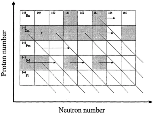
Due to its mode of production the concentration of 134CS depends essentially quadratically on the BU. The BU dependence of the concentration of lS~U is much more complex due to the fact that it is produced via many different mass chains of which five have a major importance, cf. fig. 2.3. The resulting yield curve, however, agrees decently well with a quadratic curve up to values of BU of about 40 GWdltU, fig. 2.2.

Neutron number

Figure 2.3. The main mass chains which contribute to the production Of154Eu.

The experimental arrangement is shown schematically in fig. 2.4. The fuel assembly is mounted in an elevator on the inside wall of a fuel handling pool. Gamma radiation from the assembly passes

Elevator

Figure 2.4. The experimental arrangement.

through a horizontal slit in a collimator in the pool wall, which allows the detector outside the wall to see a part of the assembly with a height of a few mm and a width equal to the diagonal of the quadratic fuel assembly.

The average gamma-ray intensity from the assembly is obtained by moving the full length of the assembly across the slit position while measuring the intensity of the radiation. Due to the rather large radial gradient of the BU of a BWR assembly, which generally is of the order of 10% between the corners, the measurement is repeated four times, once for each corner of the assembly facing the detector, and the imal intensity is obtained as the sum of these measurements.

These summed gamma-ray intensities are assumed, in a fU'St approximation, to be directly proportional to the corresponding average concentrations of fission products and thus to depend in the same way as the latter on the fuel parameters listed above. The gamma-ray intensities also depend on general circumstances such as the experimental geometry used and the specific type of assembly measured. This is taken into account by a calibration procedure, in which a number of fuel assemblies for which the BU is considered to be known, are measured.

Due to the self-absorption within the assembly, the measured intensities depend slightly on the internal structure of the assembly, i. e. how the fuel rods with different enrichment are distributed in the assembly. The latter effect has to be corrected for by calculations based on information of this distribution.

2.3

Determination of the burnup

From the measured average gamma-ray intensity of 137 Cs , the bumup can be calculated from the expression:

11

=

Kl

~e -AICT

a

~1 (Eq. 2.1)

Here 11 and Al are the intensity and the decay constant for 137CS, respectively. The bumup is denoted with

f3

and 0.1 is the correction factor for irradiation history. The coefficient Kl is a product of two factors A and B where A depends only on the geometry of the measured fuel assembly and B depends only on the geometry of the detector and collimator arrangement. The factor B is in turn a product of four factors determined by:

i) the effective area of the assembly as seen from the detector.

ii) the transmission of the radiation through the absorbing media between the fuel and the detector. iii) the solid angle covered by the part of the detector that can be seen through the collimator by the

assembly.

iv) the intrinsic efficiency of the detector 662 ke V radiation, i. e. the probability that a quantum hitting the detector will result in the storing of an event in the full energy absorption peak in the spectrunl.

The burnup of an assembly can be experimentally obtained from a gamma-ray measurement provided that the proportionality constant

K1

has been determined. Such a calibration should be carried out with great care, using as large a set of fuel assemblies as possible and least squares fitting eq. (2.1) to the data. It is clear from above that such a calibration only holds for i) the same type of fuel assembly as that to be measured and ii) using identically the same experimental geometry. The first of these two requirements is unconditional. The second requirement can be difficult to realise since the experimental conditions may change from occasion to occasion. This can be handled by measuring a reference fuel assembly at each occasion of measurement, dividing the value of

Kl

obtained with the value obtained for that particular assembly in the earlier calibration measurement, and using the ratio for correcting the count rates obtained. An other way to provide proper calibration is to use a

reference source, see section

3.4.

The expression corresponding to eq. (2.1) for the 134CS and Is~u-intensities can be written as: (Eq.2.2)

Here K is an exponent, close to 2, that is determined in a fitting procedure. The other parameters have a meaning analogous to those in eq. (2.1).

If two activities are measured, BU and eT can be obtained by combining eqs. (2.1) and (2.2). Solving for

f3

gives:

(Eq.2.3)

The coefficients of the propagation of the errors of the measured gamma-ray intensities are inversely proportional to the decay constants. This is fortunate since the accuracy is highest for the intensity of the long-lived 137Cs. It is also fortunate that the inequality /"2//"1*'K holds here since the exponent in eq. (2.3) otherwise would be inftnite.

A condition for the calculation of the burnup is that the correction factors <1j for power history can be

calculated. This is only possible if the operator can provide relevant infonnation on the power history.

If this infonnation is lacking the burnup can still be detennined but with somewhat less accuracy, see section 5.

2.4

Determination of the cooling time

The cooling time can be calculated by combining eqs. (2.1) and (2.2) and solving for CT. This results in the following expression:

eT

=

1 In{(o.

1

11)K

~}

"'-2

-KA

₁

Kl

0.2

1

2

(Eq.2.4)

The accuracy in the determination of cooling time increases with the ratio _/"2/1...1, which favours the use of 134CS and 137CS. However, the comparatively short half-life of 134CS makes it too weak to be measured at cooling times longer that about 20 years. For longer cooling times it is therefore necessary to use lS~U together with 137 Cs.

Regarding the power history correction factors <1j, the same reservations are valid here as for the burnup calculations. If these factors are not introduced the errors in the calculated cooling time increase significantly, cf. section 5.

An alternative way of determining the CT for periods less than about 20 years is to use the intensity ratio ls~ul134CS. If the exponent K and t.h.e correction factors <1j in eq. (2.2) are assumed to be equal for 134CS and lS~U, which are fair approximations, the CT can be detennined directly from the intensity ratio without further infonnation than .the values of the calibration constants K2 and K3 from

~

=

K2

e

-(A·2-A.3)CT

13

K3

(Eq.2.5)

Here index 2 and 3 indicate lS~U and 134CS, respectively.

2.5

The Power history.

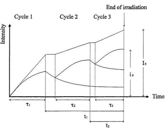
The reactors considered here are generally operated in power cycles lasting about one year including a shut-down period of 1-2 months. Figure 2.5 shows schematica1ly the yield curve of a fission product assumed to grow linearly with the BU. The yield of the isotope at the end of the final irradiation period depends, besides on the BU and the half-life of the isotope, on the number of power cycles during which the BU was acquired, and the detailed power profile of each cycle. Therefore, in order to make possible to compare on the same scale the concentrations of fission products in assemblies with different power histories, the measured gamma-ray intensities must be adequately corrected. In the present case the half-lives of the three isotopes studied are long enough to allow neglecting the detailed power distribution during a cycle. The correction is therefore limited to considers only the number of power cycles and the burnup added in each cycle as declared by the operator.

End of irradiation

Cycle 1

Cycle 2

Cycle 3

~ .~

~

Cl)

~

r

10

io

I

I

_Time

1

1

E

1

'tt _{'t2 't3}

t,

1

I J.

12

Figure 2.5. Production of a direct fission product without (dashed line) and with (full line) decay

taken into account. A correction factor

a.

is formed by the ratio IoIio.

Figure 2.5 suggests a correction factor

a.

for irradiation history as the ratio between the two cases shown in the figure. The intensity

10

in figure 2.5 can be calculated from operator declared data for each power cycle according to:

(Eq.2.6) Where f3n is the bumup acquired in cycle n.

For calculating

io

in figure 2.5 the following differential equation holds:

di

K

,,:

dt

=

IP-

l (Eq.2.7)

Here p is the power produced during each power cycle. In this treatment we assume p to be constant. The general solution of eq. (2.7) is:

. _ KIP

(1

-AI)

l - - -

-e

A

(Eq.2.8)

During each power cycle n, the fuel is irradia~ed for a period of time of "en producing the gamma intensity in. The yield

io ,

which is in summed over all power cycles, can thus be described as:

io

=KIL~(l-e-Atll)

A't n

(Eq.2.9)

In this expression we defme (3n-P"en. To take into account the decay of the fission product during the period from the end of cycle n to the end of the last cycle, in has to be multiplied by a factor e-Afn , where

to

is the period of time from the end of the n:th cycle to the end of the last cycle.

a.

= ___

-...:n~=.::....l

-L

L(1-e-

A _'tll)e-A _tll

n=l

A

't n

(Eq.2.10)

For 134CS and lS~U, where the intensity does not follow a linear relationship with bumup, the

treatment in principle becomes more complicated. However, by making some approximations one may obtain simple expressions which still provide sufficient accuracy. Assume that the intensity

10

depends on bumup as in eq. (2.11).

(Eq.2.11)

The intensity contribution ~in for each cycle can now be calculated according to: (Eq.2.12)

Here

K2

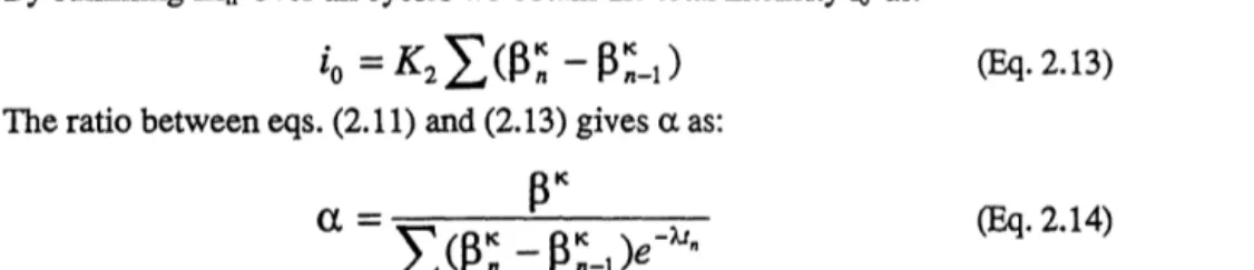
is a constant and f3n is the actual bumup at the end of cycle n. In this equation we make the assumption that all power cycles have the same duration, which is a good approximation in the assemblies studied in this report. When this assumption does not hold a more elaborate treatment is necessary in which the decay of the fission products during irradiation is taken into account.

By summing ~in over all cycles we obtain the total intensity io as:

io

=

K2L(P~

-

P~-l)

(Eq.2.13) The ratio between eqs. (2.11) and (2.13) gives

a.

as:

~K

a.

=

----=---L

(P~

-

a~-l

)e-Atll

(Eq.2.14)

Note that a. depends on the relative bumup rather than the absolute bumup at the end of cycle n. The correction factor for 137CS as calculated from eq. (2.10) for two typical cases of power history is

given in table 2.1. For 134CS and 15~U eq. (2.14) must be applied. The variations in the correction factors given in table 2.1 are seen to be much larger than for 137 Cs, which is due to the comparatively

much shorter half-lives in these cases. This relatively strong dependence of the measured gamma-ray intensities on the power history can in principle be used to verify that the power history of the fuel assembly measured is in agreement with the operators declaration.

[soto e 137es 134CS 15~U

7

cles 1.0885 1.6835 1.1722

Table 2.1. Correctionfactorsfor the three isotopes considered here, calculated for two typical power histories. The factors are independent of the B U. [n calculating the values for 134CS and 154Eu, K was set to 2 for simplicity.

2.6

The initial enrichment

In principle the initial enrichment of the fuel influences the yields of all fission products to a degree that depends 011 at fIrst hand the burnup. To investigate this effect calculations were made with

ORIGEN 2, ref. /9/ for a number of BWR assemblies with different enrichment, bumup and power history. The effect for 137CS was found to be too small to be of interest here but for 134CS and lS~U the

relative yields may vary of the order of 10% per percent enrichment for homogeneous fuel cf. figs. 2.1 and 2.2. In the fuel investigated here, the fuel pins with the highest enrichment are concentrated to the centre of the assembly which, in view of the self-absorption of the gamma radiation in the assembly, can be expected to reduce the effect of the variation of the enrichment. An detailed calculation of the total effect is rather complex because it involves a combination of bumup calculations for individual fuel pins, isotope yield calculations and self-absorption calculations. Since the assemblies investigated here do not differ much with respect to the enrichment of the fuel, a simpler, very approximate approach was adopted. The yields for 134CS and lS~U were calculated for each of the initial enrichment considered in this investigation, using ORIGEN 2. From these calculations a correction factor:

C

_i

=

1

+

f

Y3.0 - Yi

(Eq.2.15)

Yi

was fonned where

Yi

is the calculated yield for the average enrichment and burnup of the i:th assembly, Y3.0 is the yield for fuel with the enrichment 3.0%, which is used as a reference value and

the same bumup as used in Yh. An adjustable factor f is introduced in order to optimise the effect of

q.

The calculations were made for different cases of power history which, however, showed no difference in the resulting values of

Ci.

The correction for enrichment was made by applying the correction factors

Ci

to the intensities of 134CS and lS~U and, using the complete set of data, fitting

the factor f together with the parameters

K2

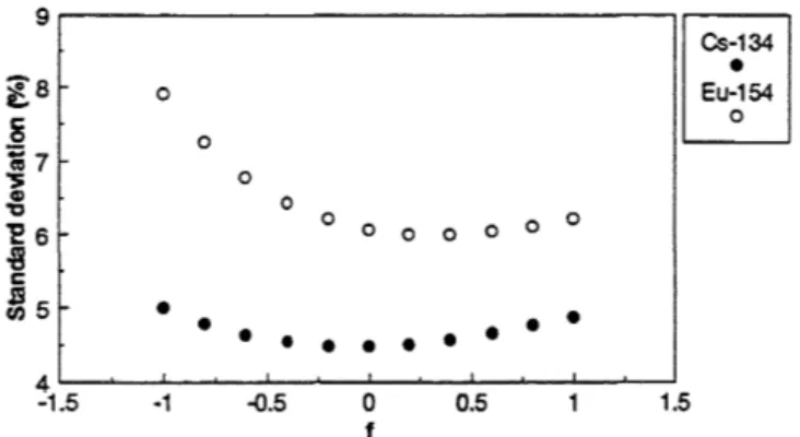
and K to obtain the best fit to eq. (2.2). The best fit was obtained for f=-O.l in 134CS and f-0.3 for IS~U, cf. fig. 2.6. In comparison with the case with no correction for enrichment, corresponding to f-o, the relative S. D. of the fits were changed from 4.6% to 4.5% in the 134CS case and from 6.1% to 6.0% in the IS~U case. The effect was more pronounced

for some of the subsets of data discussed in section

5.

9 4 -1.5 0 0

•

_•

-1 0 0

•

•

-0.5 0

•

0

•

o

f Cs-134

•

Eu-154 0 0 0 0 0 0

•

•

•

•

•

0.5 1.5

Figure 2.6. Standard deviations of individual points for the fit of 134 Cs and 154 Eu as a junction of the

parameter

f.

A minimum is obtained atf=-O.l for 134CS andf=O.3 for 154Eu.

2.7

Correction for fuel pin configuration

The gamma absorption coefficient of U02 of about 1.16 cm-I for 662 ke V gamma energy implies that radiation from fuel pins with different radial positions in an assembly contributes differently to the total radiation emitted as discussed in section 2.6. The fuel assemblies are in general designed with a radial distribution with respect to initial enrichment in order to compensate for radial differences in the thennal neutron flux. This implies that the radial distribution of the burnup will not be constant, but will in general have a gradient that may change with time. However, the radial bumup distribution tends to level out as the burn up increases.

In order to investigate the influence of these effects on the gamma-ray intensities, a two-step calculation was made. First the bumup of each fuel pin in a fuel assembly was calculated for a number of values of the total bumup of the assembly using the CASM02,3- code. In the second step these bumup values were introduced in the code cmCHA, which calculates the total gamma-ray intensity emitted from the fuel assembly considering the self absorption in the fuel assembly and absorption in the surrounding water.

The calculations were limited to 137 Cs; for the other two isotopes the calculations are more complex.

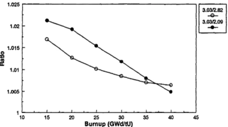
Figure 2.7 shows ratios of such calculations with three typical but different configurations corresponding to initial enrichment of 3.03%, 2:.82% and 2.06% as a function of the bumup. It is seen that the ratios only slightly deviate from the value 1.00, especially for bumup values larger than 25 GW dltU which is the region of interest in this report. Considering that the inaccuracies due to other effects generally were observed to be of the order of several percent, the experimental data were generally treated without considering this effect

1.025

r---,[±J

_3.~82 3.03f2.09 1.02 -*-1.015 o :!=I ! 1.01 1.005 15 20 25 30 35 40 45 Bumup (GWc\ltU)

Figure 2.7. Ratios between gamma intensities calculated with the code CHICHA for three fuel assemblies with different fuel pin configuration as a function of burnup. This figure illustrates that the correction for this effect is relatively small.

3

Experimental equipment

3.1

The mechanical arrangement

The mechanical arrangement of the fuel assembly and the colliInator is shown in figure 2.4. Such installations are present in all Swedish BWR plants and at the storage plant CLAB at Oskarshamn, where most of the measurements reported here have been performed.

The fuel assembly to be measured is mounted in a fixture in the elevator with a precision of the positioning of about ±1 mm in the lateral dimensions. The fixture can azimuthically be rotated 3600 manually or with the aid of a stepping motor with a precision of about 0.20.

The elevator system used to move the fuel assembly vertically has an adjustable speed control which is used to optimise the speed with respect to fuel length, scanning time etc. At the same setting of the control, the speed in the downward direction is about 20% faster than in the upward direction due to the action of gravity. However, the speed in both directions have been found to be constant within less than 1 % during scans.

When mounted in the fixture the distance between the centre of the fuel assembly and the pool wall is about 50 cm .. The transmission of gamma radiation through the water is about 1 % for 662 ke V and 3% for 1275 keY e5~u).

The collimator arrangement consists of two massive, 200 mm in diameter steel half-cylinders which sandwich a thin steel plate. The collimator hejght is defmed by a slit routed in the steel plate. The design is such that the slit width is 50 mm at the detector end and increases at the fuel end so that the - The authors are grateful to Ewa Kurcyusz at Vattenfall Fuel AB for assisting in these matters and performing the CASMO calculations.

full fuel width can be viewed by the detector. With this arrangement the slit height can be changed from 1 mm to 5 mm by interchanging slit plates. The total weight of the collimator is about 200 kg. All surfaces which defmes the slit is machined to a precision of about 20 f..U11. The length of the collimator is 120 cm and the detector is located 175 cm from the centre of the fuel assemblies.

3.2

The detector system

The requirement to detect the radiation from different isotopes separately necessitates the use of a high-resolution gamma-ray spectroscopy system based on a gennanium detector. The system should be able to measure fuel with a cooling time of several decades, when the activities of 134CS and lS~U are very weak. To measure these weak intensities in the presence of the strong intensity from 137 Cs the specifications of the system should be maximised with respect to two parameters:

i) The ratio between the peak area and the corresponding Compton area in the spectrum should be as high as possible. This generally implies the use of as large a detector as possible. Due to

economical reasons the size of the detector was limited to 40% relative efficiency.

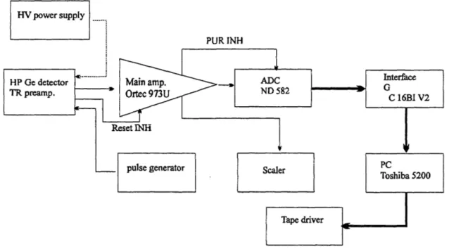
ii) The system should be able to operate efficiently at as high count rates as possible. Generally, high count rate can not be obtained simultaneously with the highest energy resolution. In the present case a high count rate is strongly preferred since the line density in the spectra is generally rather low, implying that wide energy regions around the peaks are available to defme the background with good statistics. A schematic lay-out of the detector system, is shown in figure 3.1.

The detector is irradiated radially, since it was observed that in this geometry the peak area was less sensitive to count rate variations than in a geometry with axial irradiation, ref. /10/. In general a filter of 4 or 8 mm lead is used for filtering of the otherwise strong low-energy distribution of scattered radiation. RV power supply PUR INH HP Gc detector TR preamp.

f----...

pulse generator

Figure 3.1. Schematic view of the detector system used.

ADC NO 582 Tape driver Inter:fuce G C 16BI V2 PC Toshiba 5200

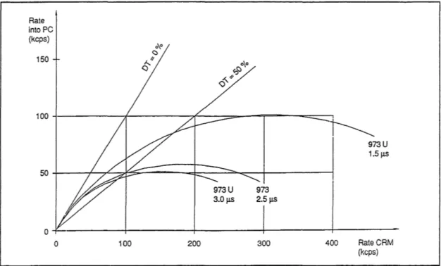
The pulses are processed by a transistor reset pre-amplifier and a gated integrator amplifier type Ortec 973 U with 1.5 JlS or 3.0 JlS integration time. The ADC is of the type ND 582 with a fixed nominal conversion time of 1.5 JlS (2.4 JlS with read-out). The digitised pulses are stored in the RAM of a PC via a fast interface card that was especially developed for the purpose. With a comparatively fast PC the throughput curves shown in figure 3.2 were obtained.

Rate into PC (kcps) 150 100~---~~---~----~--~==----~~

~

973U 1.5~

04---4---4---4---+---o

100 200 300

Figure 3.2. Throughput curves obtained/or the present detector system.

400 Rate CRM (kcps)

The energy resolution agrees decently with the values indicated by the manufacturer of the amplifier system, i. e. typically 2.5 keV FWHM: at 1332 keV using the 3 J.1S integration time option and 3.0 keV using the 1.5 J.1S integration time ..

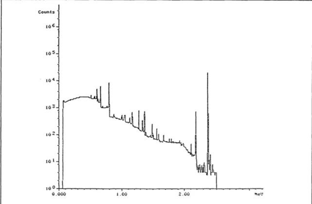
At the high count rates used, often corresponding to more than 50% dead-time, it is important to make an adequate correction for the total dead-time in the system. For this purpose the puis er-method has been employed as indicated in figure 3.3 which shows a typical energy spectrum. The pulser rate is normally adjusted to 2 kHz and the amplitude is adjusted so that the peak lies alone in the high-energy part of the spectrum.

Figure 3.3. Energy spectrum obtained with the detector system. The spectrum is recorded from a fuel assembly with BU=40.4 GWdltU and CT=672 days.

3.3

Software

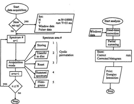
A special software package SEDAS containing a data acquisition module and an analysis module was designed for data acquisition and subsequent analysis of data. A flow chart of the main parts of the package is shown in figure 3.4.

The data acquisition module essentially performs "multi spectrum scaling", i. e. it continuously stores data from the ADC while switching the data area with regular time intervals T. The switching is performed in less than a micro second, so essentially no data are lost in the process. Three data areas are employed in cyclic permutation. During the first cycle data are stored in area #1. During the second cycle the data acquisition is directed to area #2 while the data in area #1 are transferred to the hard disc. The procedure is repeated for area #3 and area

#2,

respectively, during the third cycle, while the contents in area #1 is reset. When the data acquisition is finished, i. e. when spectrum #N has been stored, the sum of all spectra is displayed in spectrum area #4.

Set: N raN<10000 T rum 1'>55 ms Wmdowdata Pulserdata Spectrum area # 1 2 Cyclic pennutation 3 4 5 Store: Co~ct nun Co~cted histogram

Figure 3.4. Flow chart o/the software part o/the data acquisition system used/or the measurements and analysis.

Before the acquisition is started the cycle time T and the number of intervals N have to be decided. Also information on the pulser frequency and the position of the pulser peak in the spectrum have to be given as input to the subsequent dead time correction procedure. The values of N and T should be

chosen so that the product NT corresponds to the scan time of the fuel. For example, if the fuel length to be scanned is 5 m, the spatial resolution required is 1 cm and the scan time wanted is 120 s, the values of N and T are 500 and 0.24 s, respectively. For reasons of simplicity of the software, the adjustment of T can only be made in steps of 55 ms, which makes the scan time 110 s for fuel moving downwards and 137 s for fuel moving upwards if the spatial resolution should be exactly 1.00 cm. In principle there is no upper limit for N, except for the size of the hard disc used.

If the operator wants to follow the process of the data acquisition during a scan of the fuel, the net count rate in a number of peaks or other energy intervals can be monitored and displayed during the scan, provided that the energy window information has been given in the set-up procedure. The windows information needed for each peak is upper and lower limits of the regions defining the peak and the background on each side of the peak.

The net intensity of each peak is shown as a histogram displayed in spectrum area #5. An example of such histograms is shown in figure 3.5.

50 ""Co

O~-~--~----r-~-.~~-.--~-;~~-'~---'---­

o 200 600 1000 1200

Figure

3.5.

Examples of intensity distributions for 137CS, 154Eu and 60Co as recorded by the software package SEDAS. In this figure, N=250 spectra and Twas 0.88 s. Note the concentration of 60 Co in the supporting structure, especially the rod holders.

The acquisition procedure as described above relies on the assumption that the relation between the axial position of the fuel assembly and time during a scan is linear with a sufficient accuracy. If this is not the case, i. e. if the vertical movement of the assembly is irregular, the equipment must be

complemented with a position indicator. Provisions are taken in the hardware and software for counting of pulses from a positioning device and correcting the spectra accordingly.

After the scan is finished the data collected are corrected for dead-time and evaluated by the analysis module. This can be started automatically or manually. The input is a window information table and the file with N spectra obtained in the data acquisition. The analysis module corrects each of the N spectra for dead-time and creates a summed dead-time corrected spectrum and dead-time corrected histograms of the selected peaks.

The final section of the analysis module contains a routine for normalising the histograms so that each bin corresponds to the same part of the fuel assemblies independently of the direction of the movement of the assembly during recording, a routine for correcting the histograms for variations in the speed of the assembly and a routine for summing over partitions of the histograms. These partitions are usually made the same as those defmed as nodes in the operator's core physics calculations. Generally 25 evenly distributed nodes are used. Routines are also available for additional calculations such as summing over a selected number of nodes, summing over the four corners etc. Figure 3.6 shows the nodal distribution of the intensity from 137CS summed over all corners compared

- . 'en 0.. 0

-....-~ ot-' en

e

Q) +-'

e

1 400

i1. I I I I 1i I d-, I I I I I I I I I I I t I I I I I J I

1 400

- ~

-

•

Meas.

1200'--:

_-

0

Cale.

1000-

-800-

_- r

-600-

-

400

-200'--:

-~

~1200

f-~1000

~ l-

f--800

-600

-400

-200

0

~~~~~~~~~~~~~~~~~~~O

bottom

1 3 5 7 9 1 1 1 3 1 5 1 7 1 9 2 1 2 3 25

top

Node #

Figure 3.6. Experimental 137 Cs intensity distribution together with a burnup distribution based on

the operator core physics calculation. The mean values for each distribution have been used to normalise the experimental values to the calculated ones

3.4

Reference source

The results that can be obtained with the equipment described above are all based on a local calibration of the equipment, i. e. the value measured for

Kl

in eq. (2.1) is only valid in the particular experimental configuration used. In order to increase the usefulness and reliability of the results it would be valuable to be able to compare them with similar measurements obtained at other sites. This would be possible if the same assembly could be measured at different sites as discussed in section 2.3. To avoid the impractical and expensive transportation needed in such a procedure a more easily transportable reference source has been assembled, ref. /2/. It consists of a point source of about 1 Ci

137 Cs fitted into a standard BWR fuel channel, which can be placed in the same fixture as the fuel

assemblies to be measured. To simulate a vertically extended source, the 137 Cs pellet is oscillated

vertically with a constant velocity. The source need not to be extended horizontally provided that the width of the collimator slit used is constant within an accuracy of about 1 %. A further discussion is found in ref. /6/.

4

Measurements

The results reported in this paper is based on data from three measuring campaigns labelled F, G, I. The measurements took place at two different sites. Campaign F was performed at the F2 reactor at the Forsmark nuclear power plant the two other were performed at CLAB. The assemblies studied at CLAB were delivered from Forsmark 2, Barseback 1, Oskarshamn 3 and Ringhals 1.

The measurements were concentrated on BWR assemblies of the ABB Atom 8x8 type, but a few (5) assemblies of the type SVEA 64 were also measured at Forsmark 2. In total 52 BWR assemblies of the 8x8 type were measured. Of these 44 were characterised as regular, i. e. they had not been reconstructed by changing any fuel pins between the irradiation periods. In addition, 8 assemblies declared as reconstructed were measured. These assemblies are omitted in the following discussion since they are (i) too few to permit defInite conclusions and (ii) not selected in a systematical way. The latter remark is due to the fact that these assemblies in a fltSt instance were declared as regular ones. There are, however, indications that the results from the reconstructed assemblies as well as the

SVEA 64 fuel deviate slightly from the ordinary 8x8 type fuel. In the following the results and the discussion is focused on the regular 8x8 type assemblies.

Each assembly was scanned four times, once for each corner facing the detector. The number of spectra N was generally set in the range 150 to 250, corresponding to an axial resolution in the range 3.0 cm to 1.8 cm. The measuring time was typically around 1.0 s and 1.5 s per spectrum for the downward and upward movement, respectively. The collimator slit widths were 3 mm at Forsmark and 5 mm at CLAB. The detector was firmly attached to the pool wall in all measurements, since a slight translation of the detector can affect the efficiency of the detector.

With fuel in the range 20<13U<4O GWdltU and 2<Cf<8 years, total count rates in the range 20 kHz

to 50 kHz were obtained. Typically the total number of counts collected in the 137CS peak for an assembly was in the range 3.105-106, all four corners added. For the 1275 keY peak in 15~U, the intensity was typically a factor of 10-20 weaker. With these count rates the integration time constant of 3.0 us in the main amplifier could generally be used with dead-times in the range 20% to 50% and an energy resolution in the range 2.3-2.6 keY for the 60Co peaks. The energy range of the spectrum was in general about 3 MeV in order to include the 2.18 MeV gamma line from 144pr. The pulser peak was always located at the high energy region of the spectra, approximately at 2.8 MeV, where the influence of the background radiation was ~egligible.

5

Results

5.1

Procedure of evaluation and presentation

For each campaign the measured gamma-ray intensities of the 661 ke V line in 137 Cs and the 5-6 strongest lines in 134es and 15~U were evaluated and sununed over the four corners for each node as described in section 3.3. In the following, results are presented for the strongest line in each isotope,

i. e. the 661 keY line, the 795 keY line in 134CS and the 1275 keY line in 15~U summed over all 25 nodes for each assembly. Numerical results for all assemblies are given in table 5.1.

A number of alternative approaches of the summing procedure were tried. For instance, there are reasons to omit the end parts of the assemblies in the summing procedure since the core physics calculations for these parts are expected to be less accurate than for the central part, see also fig 3.6. One may also try to use higher energy transitions in 134es in order to bring down the influence of possible radial gradients the BU or to use lower en.ergy transitions in 15~U in order to obtain a self-absorption effect similar to that of the radiation from the other nuclei. However, no significant improvements over the approach taken here could be observed.

In sections 5.2 and 5.3 data are presented in two ways. In section 5.2 the intensities for each isotope have been fitted to eq. (2.1)

e

37Cs) or

eq.

(2.2)

e

37es and 15~U). Before the fit the intensities have been corrected for CT using the operator's declared values. In this procedure, which essentially is a calibration, the slope coefficient

Kx

and the exponent K have been detennined for each isotope. The evaluation has been made separately for each campaign as well as for the complete data set.

In section 5.3 results are presented from a simultaneous detemrination of BU and CT by using intensities of two isotopes according to equations (2.3) and (2.4). Here the calibration constants

Kx

and K for each isotope from section 5.2 have been used.

ReactOl' Ass.t BU eT Enrteh. No. of Cl Cl Cl Norm. Int. Int. Int. (GWd/tU) (day.) (%) cycle. (wes) ('"'Cl) ("'Eu) factOl' Wc. A<c. "'Eu

(cps) (cps) (Cl») camQ.F F2 12961 36.05 683 3.03 5 1.0589 1.4373 1.1094 1.4106 875.98 1272.36 102.97 F2 5536 14.84 2866 2.09 3 1.0448 1.3188 1.0803 1.4106 313.15 33.85 14.11 F2 12921 36.1 683 3.03 5 1.0635 1.5506 1.1310 1.4106 868.93 1155.28 101.56 F2 12922 36.1 683 3.03 5 1.0635 1.5506 1.1310 1.4106 863.29 1141.18 100.15 F2 8897 29.15 1768 2.82 4 1.0452 1.2698 1.0703 1.4106 655.93 355.47 62.07 F2 12935 34.33 264 3.03 6 1.0880 1.9259 1.2097 1.4106 836.49 1173.62 90.28 F2 8921 29.83 957 2.82 6 1.0827 1.7750 1.1796 1.4106 674.27 500.76 59.25 F2 11463 29.97 684 2.93 5 1.0669 1.6239 1.1454 1.4106 706.71 706.71 66.30 F2 12929 33.07 958 3.03 4 1.0501 1.3428 1.0872 1.4106 808.27 854.82 84.64 F2 12957 33.88 958 3.03 4 1.0502 1.3444 1.0875 1.4106 832.25 938.05 93.10 caJ'l'1Q,G B1 9330 41.1 1511 2.92 5 1.0618 1.4271 1.1106 0.7981 1001.62 775.75 95.77 B1 9329 41.1 1511 2.92 5 1.0618 1.4271 1.1106 0.7981 996.03 765.38 95.77 B1 9313 35.3 1516 2.92 4 1.0458 1.2629 1.0686 0.7981 872.32 624.91 79.81 B1 10290 32 1516 2.95 4 1.0458 1.2629 1.0686 0.7981 774.96 541.91 68.64 B1 10287 33.1 1516 2.95 4 1.0458 1.2629 1.0686 0.7981 805.28 574.63 72.63 B1 10286 32.6 1516 2.95 4 1.0458 1.2629 1.0686 0.7981 794.11 557.87 71.03 R1 5769 32.6 1903 2.75 7 1.0951 1.9138 1.2139 0.7981 726.27 259.38 58.26 F2 8962 32.4 1583 2.81 4 1.0474 1.3025 1.0781 0.7981 811.67 534.73 69.43 F2 8960 29.5 1583 2.81 4 1.0474 1.3025 1.0781 0.7981 706.32 421.40 57.46 F2 5535 19.9 1584 2.09 6 1.1148 2.1965 1.2762 0.7981 430.18 106.95 24.74 camp. I F2 12950 37.9 1277 3.05 5 1.0600 1.4575 1.1140 1.0000 901.00 806.00 91.00 F2 12952 33.2 857 3.05 6 1.0828 1.7976 1.1843 1.0000 797.00 703.00 70.00 F2 12961 36 1277 3.05 5 1.0589 1.4373 1.1094 1.0000 876.00 758.00 84.00 F2 9500 33.3 1953 2.84 5 1.0599 1.4002 1.1043 1.0000 779.00 369.00 67.00 F2 9501 30 1953 2.84 5 1.0559 1.3273 1.0882 1.0000 686.00 308.00 57.00 F2 9502 31.5 1953 2.84 5 1.0658 1.5973 1.1387 1.0000 721.00 270.00 53.00 F2 9504 31.1 1953 2.84 5 1.0719 1.7153 1.1630 1.0000 708.00 235.00 49.00 F2 9508 31.3 1953 2.84 5 1.0680 1.6242 1.1450 1.0000 711.00 259.00 53.00 F2 9510 32.1 1953 2.84 5 1.0677 1.6257 1.1450 1.0000 733.00 271.00 55.00 F2 9515 32.6 1954 2.84 5 1.0663 1.5815 1.1375 1.0000 744.00 294.00 58.00 F2 9521 29.3 1954 2.84 5 1.0668 1.5943 1.1397 1.0000 664.00 226.00 46.00 F2 9525 29.5 1954 2.84 5 1.0644 1.5568 1.1315 1.0000 687.00 247.00 49.00 F2 9529 33.6 1954 2.84 5 1.0662 1.5639 1.1352 1.0000 765.00 306.00 57.00 B1 9282 33.1 1888 2.91 5 1.0659 1.6107 1.1411 1.0000 781.00 307.00 57.00 F2 9512 35.2 1953 2.84 5 1.0578 1.3938 1.1007 1.0000 822.00 411.00 71.00 B1 9285 33 1888 2.91 5 1.0697 1.7144 1.1590 1.0000 781.00 294.00 56.00 Bl 9287 34.2 1888 2.91 5 1.0693 1.6496 1.1505 1.0000 798.00 315.00 60.00 B1 9288 31.4 2331 2.91 4 1.0466 1.3086 1.0787 1.0000 722.00 245.00 57.00 B1 9291 32.5 2332 2.91 4 1.0478 1.3256 1.0828 1.0000 769.00 265.00 62.00 B1 9292 32.1 2332 2.91 4 1.0468 1.3003 1.0776 1.0000 763.00 270.00 62.00 B1 9295 35.9 1889 2.91 5 1.0690 1.6253 1.1473 1.0000 837.00 347.00 64.00 B1 9297 34 1889 2.91 5 1.0692 1.6460 1.1497 1.0000 819.00 323.00 58.00 B1 9302 35.6 1889 2.91 5 1.0687 1.6376 1.1486 1.0000 827.00 340.00 63.00 B1 10287 33.1 1889 2.95 4 1.0458 1.2629 1.0686 1.0000 790.00 412.00 67.00

Table 5.1. Declared data for the fuel assemblies considered in this work together with measured

gamma-ray intensities, normalised to campaign I and correction factors for power history. The measured gamma-ray intensities are not corrcted for cooling time nor power history.

5.2

Determination of the calibration constants

Kx

and

K

5.2.1

137CS

For each assembly measured a data point (I,~) was defined with

1= 1

₁0. leA-ICT (Eq.5.1)

Here 11 is the measured gamma-ray intensity of the 137 Cs line and CT is the operators' declared value. The correction factor (It is calculated using eq. (2.10) and the operators' declared data. For each

campaign a straight line

I-KR

_{- 11-'} (Eq.5.2) was fitted to the data points. Figure 5.1 shows an example of such a fit.

1,400

r - - - ,

1,200

i

.2. 1,000 ~ _en 800 j .5 600 ~ ~ 400 200 10 20 30 40 50

Declared bumup (GWdltU)

Figure 5.1. Measured intensities from 137 Cs, corrected for cooling time and power history, v. s.

burnup. The line is a least squares fit to the data.

The slope coefficient

Kt

with standard deviation (S. D.) and the S. D. for the individual points are given for the three campaigns and the summed data in table 5.2. One may first observe that the values of

Kt

obtained in the three campaigns agree well enough to suggest that the three sets of data can be added for a common fit, which yields an S. D. of the individual points of 2.7%. This value is of interest since it directly gives the relative uncertainty of the BU as measured with the HRGS method. The magnitude of this uncertainty is influenced by a number of effects or circumstances which will be discussed in the following:

1. Counting statistics. Typically 105-106 counts have been collected for the t37CS peak, implying a

contribution in the range 0.1-0.3% to the error.

2. Systematic experimental errors. A number of possible sources of systematic errors have been investigated, refs. 16,101. The errors that may influence the results given in table 5.2 are all estimated to be less than 1 %.

To check the reproducibility of the measurements all fuel assemblies studied in campaign F were measured twice. The average difference between the two measurements was 0.6%. Another indication on the degree of reliability of the measurements is obtained from the measurements of fuel assemblies with symmetric positions in the core, which are expected to have identical values of BU. Three such pairs have been measured and show pairwise an agreement within 1 % of the gamma intensity.

3. Uncertainty in the declared BU. The accuracy of the BU values obtained in the core physics calculations is not very well known. Rather large uncertainties are known to exist for the parts of the fuel subject to large void coefficients (cf. fig 3.6), and some uncertainty is also expected in the earliest power cycles of the fuel. At the end of the fuel cycle, however, these uncertainties can be assumed to level out and the declared BU values generally seem to be believed by the core

physicists to be accurate within 2-5%. One may observe that this estimate agrees well with the S. D. values given in table 5.2. This line also shows that the S. D. value obtained for each campaign is somewhat smaller than that obtained for the complete set of data. This is even more clear if data for a particular reactor are singled out One such case is shown in the table, for Forsmark 2, which also shows a significantly (-4%) smaller value of the slope coefficient K1 than the campaigns performed at CLAB. It may in this case be questioned whether the fact that the measurements were performed at different sites may introduce any systematic errors. This is not likely here since the Forsmark data were normalised to those at CLAB by measuring the same fuel assembly at both places, thereby eliminating the possible sources of error that could be associated with the use of the reference source. Similar results of small (a few percent) but significant deviations between slope coefficients for fuel from different reactors measured in the same campaign have been obtained in the CLAB measurements.

The S. D. of the slope coefficient K1 depends somewhat on the homogeneity of the data set. For example, in campaign F there were three assemblies measured which had a low BU and an extraordinary irradiation history. They originate from the initial core of the F2 reactor and was in operation during three and seven cycles with a final bumup of 21.8 and 22.6 GWdltU, respectively. The K1 value obtained with these assemblies included in the analysis for campaign F is 26.58±O.18. Also the S. D. of the 137CS data points increase from 1.72% to 2.98%.

4. Possible fundamental uncertainties of the method

As discussed in section 2.5 the gradient of the BU in BWR fuel assemblies in combination with the self absorption of gamma-rays in the fuel assembly may give rise to systematic effects. From calculations they are estimated to be of the order of ±l % in the BU range 20-40 GWdltU. An other possible source of error would be a varying degree of radial redistribution of the Caesium within the fuel pins. However, assuming a maximal axially symmetric redistribution within each fuel pin, this would affect the measured intensities less than 5%.

The lower part of table 5.2 is based on the same data as the upper part with the difference that the data have not been corrected for power history. For the slope coefficient of the 137CS intensity it is seen that neglecting the power history correction does not impair the results significantly. This is expected in view of the long half-life of 137CS.

5.2.2

134CS

and

lS4Eu

In analogy with the procedure described in section 5.2.1, a data point (I,~) was calculated from

/ =

/2u2e/..2CI' (Eq.5.3)

where ~ is the experimentally observed count rate on the 795 keY and 1275 keY transitions in 134CS and 1S~U, respectively, CT is the operator's declared CT and ~ is the correction factor for power history as calculated from eq. (2.9). A fit of the data points from all campaigns to the exponential of eq. (2.2) is shown in figs. 5.2 and 5.3. The fitting parameters K2 and K from this fit and for the fits of each campaign are given in table 5.2. As expected the parameter K is found to be close to 2 for 134CS, while for 1S~U a lower value is found.

The parameters fitted agree well within the errors for the different campaigns but the variation of K2 is sometimes rather large, up to 50% ,which is much more than might be expected from the variation in the data points. This is due to the rather strong coupling of the two fitting parameters, which lead to a good fit of the data for a rather large variety of combinations of the parameters.

5,OOOr---r---~

8:

4,000

e

~ "in 3,000 j c ~ 2,000

~

1,000 10 20 30 40 50

Declared bumup (GWdltU)

Figure 5.2. Measured intensities from 134CS corrected for cooling time, power history and initial enrichment v. s. burnup. The curve is a least squares fit to the data.

200r---~

10 20 30 40 50

Declared bumup (GWdltU)

Figure 5.3. Same as infig. 5.2 but for 154Eu.

The relative S. D. of the individual points is larger than for 137CS by a factor of 1.7 for 134CS and a factor of 2.2 for

lS"Eu.

It has not been possible within the economic limits of this work to deduce the reason for this, but besides the list of sources of errors given in section 5.2.1 some additional error sources may be mentioned:

Uncertainty in the correction for power history. The half-lives for 134CS and lS~U are both comparable or shorter than the fuel cycle, which makes the correction for power history much more important than for 137CS. This can be inferred from the lower part of table 5.2, which shows the values of the coefficients obtained from data points that have not been corrected for power history. One observes that the values for 134es and lS"Eu given in this part of the table have much larger uncertainties and vary much more relative to the parameters based on the corrected data than do the values for 137 Cs. In perfonning the correction, from power history, eq. (2.9), only corrections down to a time scale of one whole power cycle were considered. It is likely, especially for 134Cs, that one would obtain a smaller S. D. of the fit if the power history could be corrected for in more detail. Another possible source of error is that in the correction function, eq. (2.14), for practical reasons, the time-dependence of the activity during irradiation was not given its exact form but approximated with a simpler function. Calculations perfonned with different functions showed however that this part of the correction was not important for the fit.

Uncertainty in the form of the fitted function. The data points of lS~U in general give a fit with a S. D. of more than a factor 2 larger than that obtained for the corresponding data for 134CS. The main reason for this is not clear, but it should be observed that while the function fitted to the 134CS points theoretically should be very close to a quadratic function, the function fitted to the lS~U data is only a first approximation of a more complex function, that may vary between different positions in the core and different axial positions in the assembly.

The possibility to improve the fit by using data from only a limited axial part of the assemblies was investigated. For all three isotopes the evaluation of the data and the fit to eqs. (2.1) and (2.2) were

repeated using only the intensities measured between the nodes #9-17. No improvement of the fits were observed.

Influence of original enrichment. The influence of the enrichment on the intensities measured have only been treated approximately for these isotopes, see section 2. It is possible that a more accurate treatment could lead to a better fit of the data.

5.3

Simultaneous determination of BU and CT

Provided that the corresponding calibration parameters

Kx

and K are known, eqs. (2.3 and (2.4) can

be used to determine BU and CT from measured intensities of two isotopes, i. e. 137es and 134es or 137CS and 15~U. The results of such calculations are demonstrated in the following under two different circumstances: (i) Information on power history is available. (ii) No information on the assembly is available. Case (i) corresponds to a,procedure of verification of the fuel parameters, while case (ii) corresponds to an independent measurement of the parameters. The accuracy in case (ii) is however considerably worse than in case (i).

Data points corrected I)

Campaign F G I F+G+I

No. of ass. 10 10 24 44

KI

e

37Cs) 26.73±O.14 28.12±O.16 27.92±O.10 27.71±O.1l S. D.ct37Csl (%) 1.72 2.34 1.75 2.68 K2

e

34Cs) 3.43±O.69 2. 24±O.46 3.18±1.63 2.83±O.42 S. D.e34C~ (%) 4.45 3.37 4.39 4.47

K (I34CS) 1.91±O.06 2.05±O.06 1.95±O.15 1.98±O.04 K2 (IS4Eu) _{0.48±O.13 0.54±O.05 0.57±O.41 0.55±O.11} S. D. (IS4Eu) (%) 5.93 1.66 6.10 5.98

K

e

S4Eu) 1.56±O.08 1.52±O.03 1.49±O.21 1.51±O.06 Data points not corrected

Campai2n F G I F+G+I

No. of ass. 10 10 24 44

KI

e

37Cs) 25. 16±O. 19 26.59±O.26 26.27±O.11 26.11±O.12 S. D.

e

37Cs) (%) 2.45 4.54 2.16 3.43 K2

e

34Cs) 4.50±3.43 0.23±O.24 2.52±4.13 1.56±O.86 S. D. e34Cs) (%) 17.60 18.05 13.80 17.42

K

e34Cs) 1.72±O.22 2.60±0.30 1.89±O.47 2.03±O.16 K2

e

S4Eu) 0.32±O.13 0.16±O.06 0.44±O.45 O.28±O.08 S. D.

e

S4Eu} (%} 9.21 6.20 8.63 8.89

Ke

S4_{Eu) 1.65±O.12 1.84±O.11 1.53±O.29}

1.67±0.08 1) The data points have been corrected for power history according to eqs. (2.10) and (2.14). Also a correction was made for initial enrichment

in the cases of 134CS and 15~u. See text for further details.

Table 5.2. Results of the calibration procedure for each campaign and the grand total of all campaigns.

5.3.1

134CS

and

137CS

Fig 5.3.1a and b shows the agreement between the experimentally obtained BU and CT, respectively and the declared values for case (i). The corresponding diagrams for case (ii) is shown in fig 5.3.2a and b. Standard deviations for data sets are given in table 5.3.

As expected the S. D. of the BU in case (i) is about the same as that obtained for 137 Cs in the

calibration fit, section 5.2.1. In this case the CT can be verified within two months.

In case (ii), the BU can still be obtained with about 3% S. D., while the uncertainty of the CT has increased to about 6 months. These numbers are in principle not sensitive to the duration of the CT up to about 20 years, when the decay of 134CS starts causing large statistical uncertainties.

-=

40

-

"C

;:

e.

g-

30

c

...

:s

.c

~

20

Cl) E "t: Cl)

~10

10

20

30

40

50-Declared burnup (GWd/tU)

~S'

.-

_~

_3,000

+=

en

.s

"0

8

2,000

S

~

.t:

!.

1,000

><

w

1,000 2,000 3,000 4,000

Declared cooling time

(cl)

Figure 5.3.1. a) Experimentally obtained burnup v. s. declared burnup. b) Cooling time determined experimentally

v. s.

declared cooling time. In both cases the information on power history is available. The line in the figure corresponds to a least squares fit of the experimentally obtained values to the declared ones.

50---~

-=

40

;;

~

g-

30

c

...

:s

.c

~

20

Cl) E "t: CD ~ ~

10

10

20

30

40

50

Declared burnup (GWd/tU)

4,000 - - - .

~3,OOO

~

~

en

c

1

2,000

I

!

1,000

+

1,000 2,000 3,000 4,000

Declared cooling time

(cl)

Figure 5.3.2. Same as in fig. 5.3.1 but for the case where no information on the power history is available.

5.3.2

154Eu

and

137

Cs

Figs. 5.3.3 and 5.3.4 show the agreement ofBU and

er

for the combination lS~U

+

137CS in analogy with figs. 5.3.1 and 5.3.2. The corresponding S. D. are given in table 5.3.

The numbers given for case (H) imply that these data allow the measurement of BU with an accuracy of about 6%, while the CT cannot be determined within better than about 2 years. No significant improvement is observed for the corrected data.

It was noted in section 5.2 that the data for lS~U scatter more than for the other isotopes. The explanation for this can be found by differentiating eqs. (2.3) and (2.4) with respect to

h

and re-arranging:

Eq. (5.4) and

Eq. (5.5)

From eq. (5.4) we conclude that the relative uncertainty in ~ is equal to the relative uncertainty in the 134CS or lS~U intensities. It is inferred from table 5.3 that the relative uncertainty of the 15~U intensities is roughly a factor of 2 larger than for the 134CS -intensities.

The uncertainty in CT, eq. (5.5), is largely dependent on the constant factor C which, in turn, is dependent on the specific values of the decay constants. For lS~U C= 7796 days and for 134CS C= 1253 days i. e. a factor of 6 smaller in this case.

We conclude that the uncertainties discussed above implies that the total uncertainty in CT for the combination of 137CS +lS~U is a factor of 12 larger than for the corresponding value for 137CS

+

134Cs.

This result is supported by the results given in table 5.2.

5.4

Determination of

CT

from the ratio

154Eu/134CS

As pointed out in section 2.4, an alternative way of obtaining CT independently is to use eq. (2.5). In figure 5.4 we show a plot where the ratio between the uncorrected intensities of 15~U /134CS are plotted v. s. cooling time. The curve in fig. 5.4 is a least squares fit of the fonn:

R

=

Ae

-CTO .. 2_-A3) Eq. (5.6)

Where

A2

and A,3 corresponds to the decay constants for lS~U and 134CS, respectively and A is a fitting parameter. The S. D. of the ratio corresponds to a S. D. in cooling time of 170 days.

This method of determining cooling time can be used up to about 20 years of cooling time due to the same arguments as discussed in section 2.4.

Data points corrected

l) Campai2n F G I F+G+I No. of ass. 10 10 24 44 AB

e

37Cs) (%) 1.72 2.34 1.75 2.68 AB ct34CS}{ %1 1.87 2.63 1.92 2.93 AB (lS4Eu) (%) 3.14 3.91 3.79 5.56 ACT e34Cs) (d) 58 61 56 62 ACT eS4Eu) (d) 416 278 477 565

Data points not corrected

Campaign F G I F+G+I No. of ass. 10 10 24 44 AB

e

37Cs) (%) 1.88 4.37 2.06 3.20 AB ctS4Eu) (%) 2.90 6.82 3.81 6.21 ACT e34Cs) (d) 167 179 152 170 ACT eS4Eu) (d) 514 560 564 698 1) The data points have been corrected in the same way as in table 5.2.

Table 5.3. Results of the burnup and cooling time verifications. The upper part corresponds to data corrected for power history and initial enrichment. The lower part corresponds to a situation where no declared parameters are available.

50~---~

_{4,00J , - - - ,}

'B'3,00J

...

+

~

=

_~

~

2,(XXJ

11,(XXJ

I

o~--~---~ 10 20 30 40 50

o

1,(XX) 2,00J 3,000 4,000

Declared bumup (GWd/tU)

Declared

cooling

time

(d)

10 20 30 40 50

Declared burnup (GWdltU)

4,000 . . . - - - .

-:5!.

~ 3,000 ;::a en .5

g

2,000 Cl

S

i

~ 1,000 Cl) Q. )( W

+

Of-J---:---I

o

1 ,000 2,000 3,000 4,000

Declared cooling time (d)

Figure 5.3.4. Same as in fig. 5.3.3 but for the case where no information on the power history is available.

0 . 5 . - - - ,

500 1,000 1,500 2,000 2,500

Declared cooling time (days)

+

3,000

Figure 5.4. Plot showing the ratio 154Eu /134CS v. s. declared cooling time. The curve is a least squaresfit and the corresponding S. D. o/the data points is 170 days.

6

Discussion

The results presented in section 5 fonn a basis of a discussion of the practicability of the HRGS method for safeguard induced measurements on BWR fuel. It may be stated in general that, provided the proper equipment is installed, the HRGS method is both fast and accurate. Typical measurement times are 15 min per assembly. An estimation gives that for fuel up to about 20 years of age, bumup and cooling time can be verified at a level of 2-3% S. D. and a few months, respectively. For older fuel, with up to about 50 years cooling time, the latter can be verified at a level of accuracy of about 1.5 years S. D.

The present experiments have utilised existing.elevator and collimator installations. This is however no necessary requirement, similar measurements have been made using a fuel handling machine instead of an elevator and a transportable underwater installation including a collimator and a Ge

detector /111.

In section 2.1 five fuel parameters were listed of which three have been treated extensively in this report. One of the remaining two parameters, the initial enrichment of the fuel, has only been studied theoretically, since essentially all assemblies measured here has very nearly the same average enrichment. It remains to verify experimentally the calculations reported in section 2.