2015:48 Technical Note, Supplementary review of SKB’s further RFI response

(1)

Technical Note

Supplementary review of SKB’s

further RFI response

Main Review Phase

2015:48

Authors: Richard Kłos

(2)

(3)

SSM:s perspektiv

Bakgrund

Strålsäkerhetsmyndigheten (SSM) granskar Svensk

Kärnbränslehanter-ing AB:s (SKB) ansöknKärnbränslehanter-ingar enligt lagen (1984:3) om kärnteknisk

verk-samhet om uppförande, innehav och drift av ett slutförvar för använt

kärnbränsle och av en inkapslingsanläggning. Som en del i granskningen

ger SSM konsulter uppdrag för att inhämta information och göra

expert-bedömningar i avgränsade frågor. I SSM:s Technical note-serie

rap-porteras resultaten från dessa konsultuppdrag.

Projektets syfte

Det övergripande syftet med projektet är att granska SKB:s svar på den

kompletterande information som begärts av SSM om härledning av

flödesrelaterade parametrar. Parametrarna härleds från ythydrologisk

modellering och används i radionuklidtransport- och

dosberäkn-ingsmodellerna.

Författarn sammanfattning as

Som en del i SSM:s granskningsprocess för SKB:s ansökan om licens

för att bygga ett djupt geologiskt slutförvar för använt kärnbränsle i

Forsmark (SR-Site) har SSM begärt ytterligare information (”requests

for further information”, RFI) av SKB. Denna kompletterande rapport

behandlar SKB:s slutliga svar på RFI om modelleringsfrågor av

radio-nuklidtransport i biosfären som SSM fick i juni 2015.

Radionuklidtransport- och dosberäkningsmodellen i SR-Site är baserad

på en hydrologisk modell som i sin tur är baserad på detaljerad

plat-skarakterisering. Av intresse i denna del av granskningen är det

för-farande genom vilket den detaljerade platsbeskrivande modelleringen

översätts till hur hydrologin utvecklas med tiden i

radionuklidtransport-modellen. Det är flera steg i detta förfarande, vart och ett med

till-hörande approximationer och förenklingar.

I rapporten jämförs den detaljerade beskrivningen av hydrologin i det

“genomsnittliga objektet” (det så kallade referensfallet), som används av

SKB för att approximera generiska hydrologiska egenskaper för

avrin-ningsområdet i det framtida Forsmarkslandskapet, med strukturen och

den algebraiska beskrivningen av flödena i

radionuklidtransportmodel-len. Motiveringen till modelleringsförenklingarna som SKB har

genom-fört i detta förfarande undersöks. Den implementerade hydrologin i

radionuklidtransportmodellen har tydliga skillnader jämfört med det

“genomsnittliga objektets” hydrologi.

För att undersöka effekterna av dessa skillnader på beräknade doser

i radionuklidtransport- och dosberäkningsmodellen presenteras en

uppsättning resultat som jämför fördelningen av radionuklider i den

modellerade biosfären. Tre olika implementeringar av radionuklid-

transportmodellen utvärderas, var och en med en egen tolkning

av hydrologin:

(4)

• modellen med vattenflöden som tagits direkt från det “genomsnittliga

objektet” - referensfallet,

• modellen med vattenflöden som härletts från SKB:s algebraiska approx

imation av det “genomsnittliga objektet”, och

• modellen med objektspecifika vattenflöden för valda avrinnings-

området tagna från den detaljerade hydrologiska modellen av

Forsmarksområdet.

Resultaten tyder på att doserna som beräknats från den algebraiska

abstraktionen av det “genomsnittliga objektet” skulle likna de doser

som fås om vid ett fullständigt genomförande av det “genomsnittliga

objektets” hydrologi, trots att flödessystemen är olika till sin struktur.

Det finns en liten icke-konservativ bias i SKB:s

radionuklidtransport-modell för svagare sorberande radionuklider.

När SKB:s radionuklidtransportmodell jämförs med flöden från specifika

objekt visar resultaten större avvikelser. Det är därför tydligt att

använd-ningen av det “genomsnittliga objektet” i SR-Site inte ger en adekvat

rep-resentation av viktiga aspekter av hydrologi i radionuklidtransport- och

dosberäkningsmodellerna.

Resultaten innebär inte nödvändigtvis ett ogiltigförklarande av de

resul-tat som presenteras i SR-Site, men visar att för framtida

biosfärsmodel-lering, skulle förtroendet för modelleringen kunna förbättras genom en

bättre beskrivning av radionuklidtransport och ackumulation i

radio-nuklidtransport- och dosberäkningsmodellerna.

Project information

Kontaktperson på SSM: Shulan Xu

Diarienummer ramavtal: SSM2011-592

Diarienummer avrop: SSM2014-1147

Aktivitetsnummer: 3030012-4401

(5)

SSM perspective

Background

The Swedish Radiation Safety Authority (SSM) reviews the Swedish

Nuclear Fuel Company’s (SKB) applications under the Act on Nuclear

Activities (SFS 1984:3) for the construction and operation of a

reposi-tory for spent nuclear fuel and for an encapsulation facility. As part of

the review, SSM commissions consultants to carry out work in order to

obtain information and provide expert opinion on specific issues. The

results from the consultants’ tasks are reported in SSM’s Technical Note

series.

Objective

The general objective of the project is to review SKB’s response to the

complementary information requested by SSM regarding the derivation

of flow related parameters. The parameters are derived from surface

hydrological modelling and used in the biosphere radionuclide

trans-port model.

Summary by the authors

As part of the review process implemented by SSM in respect of SKB’s

license application for construction of a deep geologic final repository

for spent nuclear fuel at Forsmark (SR-Site) a number of requests for

further information (RFIs) were submitted by SSM to SKB. This

sup-plementary report deals with SKB’s final response to the biosphere and

dose assessment modelling RFIs that was received in June 2015.

The dose assessment modelling in SR-Site is based on a hydrological

model that is itself based on detailed site characterisation. Of interest

in this part of the review is the procedure by which the detailed site

descriptive modelling is translated into the representation of evolving

hydrology used in the radionuclide transport sub-model of the dose

assessment model. There several steps in this procedure, each with

asso-ciated approximations and simplifications.

This report compares the detailed description of the hydrology of

the “average object” (known as the reference case) as used by SKB to

approximate generic hydrological characteristics of basins in the future

Forsmark landscape, with the structure and algebraic description of the

fluxes in the radionuclide transport model. The justification of the

mod-elling simplifications implemented by SKB in this procedure are

exam-ined. The implementation of hydrology in the radionuclide transport

model has clear differences when compared to the reference “average

object” hydrology.

To examine the impact of these differences on calculated doses in the

dose assessment model a set of results are presented that compare the

distribution of radionuclides in the modelled biosphere. Three

differ-ent implemdiffer-entations of the radionuclide transport model are evaluated,

each with a different interpretation of the hydrology:

(6)

• the model using water fluxes taken directly from the “average object” –

the reference case,

• the model using water fluxes derived from SKB’s algebraic approxima

tion of the “average object”, and

• the model using object specific water fluxes for selected basins taken

from the detailed hydrological model of the Forsmark region.

Results indicate that the doses calculated from the algebraic abstraction

of the “average object” would be similar to those from the full

implemen-tation of the “average object” hydrology, despite the flow systems being

different in structure. There is a slight non-conservative bias in the SKB

radionuclide transport model for the more weakly sorbing radionuclides.

When the SKB radionuclide transport model is compared with to full flux

maps from specific objects the results show greater discrepancies. It is

therefore clear the use of the “average object” in SR-Site does not give

an adequate representation of key aspects of the hydrology in respect of

dose assessment calculations.

The results do not necessarily invalidate the results presented in SR-Site

but indicate that, for future assessments, confidence in the modelling

would be enhanced by a better description of radionuclide transport and

accumulation in the dose assessment model.

Project information

(7)

2015:48

Authors: Richard Kłos 1)_{, Anders Wörman}2)

1) _{Aleksandria Sciences Ltd, Sheffield, United Kingdom}

2)_{KTH, Stockholm, Sweden}

Supplementary review of SKB’s

further RFI response

Main Review Phase

(8)

This report was commissioned by the Swedish Radiation Safety Authority

(SSM). The conclusions and viewpoints presented in the report are those

of the author(s) and do not necessarily coincide with those of SSM.

(9)

1. Introduction and overview

This note gives a supplementary review of material provided by SKB on 19-05-2015 (SKB, 2015ab), following the completion of the final report on the SR-Site. The ma-terial deals with the response to the Requests for Further Information (RFI, see Ap-pendix 1). SKB’s initial response dealt with Request 1 and was received in July 2014. The new material relates to the procedure for estimating water fluxes and as-sociated transfer rate coefficients in the Avila et al. (2010) dose assessment model. The request is formulated as:

Please provide detailed step-by-step description of the procedure used to justify, de-fine and calculate the numerical values used in the radionuclide transport (RNT) model for the following six parameters:

i) Upwards velocity out of lower regolith: adv_low_mid;

ii) Fraction of flow from lower regolith directed to mire: fract_mire; iii) Net precipitation: runoff;

iv) Fraction of infiltration to catchment moving laterally in terrestrial subsystem: Ter_adv_midup_norm

v) Fraction of infiltration to catchment moving laterally in aquatic subsystem: Aqu_adv_midup_norm

vi) Fractional lateral flux from subcatchment to wetland: flooding_coef

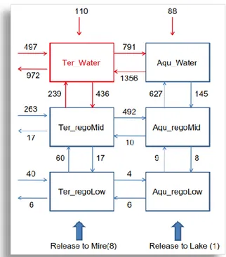
The hydrological information provided by SKB in the SR-Site documentation is in the form of the “average object” from Bosson et al. (2010). The numerical values are shown in Figure 1. These are translated into the algebraic expressions for the fluxes for indicated in Figure 2. This is the representation of the water fluxes in-cluded in the Pandora1_{model. This document goes some way to explain how the}

model used in the dose calculations (with water fluxes expressed in Figure 2) is re-lated to the hydrological basis of the “average object” shown in Figure 1.

The issue addressed in SKB’s response is the relationship between the numerical values in Figure 1 and the algebraic expressions for the parameters in Figure 2. The expressions and parameters are listed in Table 1. It is the relationship and, specifi-cally, the justification of Table 1 and Figure 2 on the basis of Figure 1 that was the prompt for the RFI. The explanation in Avila et al. was insufficient.

There are three stages in understanding how the “average object” numerical data are used in the SR-Site model:

1. Translation of the flux map in Figure 1 to the fluxes as modelled in Figure 2. Clearly not all the fluxes identified in the “average object” are imple-mented in the dose model.

2. Assignment of numerical values from the “average object” fluxes to the fluxes in the transport model.

3. Derivation of the normalised fluxes that are used in the Avila et al. model itself. Step 2 uses fluxes as numerical values in mm year-1_{, the transport}

model (known as the “Pandora model” in SKB, 2015a) uses one absolute flux (adv low mid_ _ m year-1_{) and four normalised values (}

mire fract ,

flood

f , Ter adv mid up norm and_ _ _ _ Aqu adv mid up norm ). _ _ _ _

These addressed in the analysis section, that follows. Numerical implications follow in Section 3.

(12)

Figure 1. Advective fluxes (Fij) for an average lake-mire object obtained from the MIKE SHE simulations. Values of area normalized fluxes are given in units of mm/year (SKB, 2015a).

Figure 2. Conceptual representation of the water fluxes included in the Pandora imple-mentation of the SR-Site radionuclide transport model (RNT - SKB, 2015a). These are the fluxes as used in the RNT and are denoted in the analysis here as Φij. The algebraic

(13)

Table 1. Summary of algebraic expression for the water fluxes in the Avila et al. (2010) ra-dionuclide transport model shown in Figure 2 (SKB, 2015a). Numerical values are quoted in Table 2 of SKB (2015a).

Water flux, Φij in RNT

model Parameterisation / description

Flux from Mire to Lake TerUp



1 flood



* catch*

AquWat _obj area f runoff area    

Flux from Lake to Mire AquWat flood* catch*

TerUp _obj area f runoff area   

Flux from Regolith Mid TerMid _ _ _ _ * catch*

TerUp _obj

area

Ter adv mid up norm runoff

area



 

Flux between water and

sediment _ _ _ _ * *

catch AquMid

AquUp _obj

area

Aqu adv mid up norm runoff

area



 

Flux downstream from lake AquWat watershed*

Downstream _obj area runoff area   

Flux from Regolith Low to

Mire LowTerMid fractmire*adv low mid_ _

 

Flux from Regolith Low to

Lake





1 * _ _

Low mire

AquMid

fract adv low mid



  

_ _

adv low mid is the area normalized total advective flux from the rego_low to the Ter_rego_mid and Aqu_rego_mid (m/y)

= 0.044 m year-1

mire

fract is the fraction of the advective flux from the rego_low that _{goes to the mire (-)}

= 0.98 unitless

_ _ _ _

Ter adv mid up norm

is the advective flux in the terrestrial object from the rego_mid to the rego_up normalized by the net lateral advective fluxes from the mire (-)

= 0.30 unitless

_ _ _ _

Aqu adv mid up norm

is the advective flux in the aquatic object between the rego_mid and the rego_up and between the rego_up and the water normalized by the net lateral advective fluxes from the mire (-)

= 0.64 unitless

flood

f is a coefficient used to calculate the flux from the lake to _{the mire by flooding (-)}

(14)

2. Analysis

2.1. Mapping the “average object” to the RNT model

Figure 3 provides a side-by-side comparison of the Bosson et al. (2010) “average object” and the Avila et al. (2010) RNT model. This emphasises the differences – there are missing compartments, additional compartments, combined compartments as well as missing fluxes. Making sense of the translation of water fluxes from “av-erage object” to RNT model is the aim. Kłos et al. (2014) have covered this material already (that analysis was the reason for the RFI in the first place) but there is addi-tional material in SKB (2015a).

In brief, there is not a single compartment-to-compartment interaction in the “aver-age object” that has a direct correspondence in the RNT model. Only the two mid-regolith layers are common, one each for the terrestrial and aquatic sub-models. There is no interaction between the terrestrial and aquatic mid and upper regolith. In contract there is “instantaneous” interaction between the lower regolith in the aquatic and terrestrial systems – ie contents of these compartments are combined.

“Average object” RNT model

Figure 3. Comparison of compartment and fluxes: Bosson et al. (2010) “average object” (left) and Avila et al. (2010) RNT model (right). With reference to the “average object”, the cross-hatched compartment is not included in the RNT model, dotted fluxes are not in-cluded in the RNT model. With reference to the RNT model, the compartments denoted by red text are not present in the “average object”, and the purple regolith low compart-ment is an amalgamation of the two lower regolith compartcompart-ments. Dashed fluxes are im-plied from the “average object” and the red fluxes are the inputs of radionuclides.

Ter_rego Low Ter_rego Mid Aqu_rego Low Ter_water Aqu_water Aqu_rego Mid Rego Low Ter_rego Up Aqu_rego Up Aqu_water Ter_rego Mid Aqu_rego Mid

(15)

2.2. Combining fluxes from the “average object”

How the fluxes in the “average object” are combined to generate the RNT model pa-rameterisation is crucial to understanding and building confidence in the SR-Site dose assessment model. Because the mapping outlined above is so obscure the usage of the water fluxes in from the “average object” is now addressed in detail.

In the RNT model a total of 10 fluxes are defined. These are considered in turn us-ing the fluxes from the “average object” in Figure 1.

1. Flux from lower regolith to mire

This is the balance between the upwards and downwards fluxes from the terres-trial lower regolith and the terresterres-trial mid-regolith (purple arrows):

60 17 43

Low TerLow TerMid TerMid TerMid TerLow

F F

  

  

   mm year

-1 ₍₁₎

This is at least clear, it is the net up-ward flux from the terrestrial lower regolith.

2. Flux from lower regolith low to lake

Similarly this is the net upward flux between the compartments on the aquatic side of the flux map (blue ar-rows):

9 8 1

Low AquLow AquMid AquMid AquMid AquLow

F F

  

  

   mm year

-1_. ₍₂₎

By combining the two lower regolith compartments, SKB treat the exchange be-tween them as, effectively, instantaneous. The total net inflow to the lower rego-lith is 44 mm year-1_{(see Kłos et al. 2014 for the analysis). Most of this flow}

arises from the subcatchment and only a small fraction from the bedrock with the mire receiving the majority of the flow. Mixing between the two lower regolith domains is indicated as being relatively slow. The combination of the two layers is not well motivated but may not have significance for the dose modelling.

3. Total flux out of the mid-regolith

According to SKB (2015a), the flux from the terrestrial mid-regolith to the terrestrial upper regolith (TerMid to TerUp) is as shown. It combines the net lateral exchange with the aquatic mid regolith and the inflow from the terrestrial water compartment less the loss to the lower regolith. It neglects the input from the subcatchment as well as the input from the lower rego-lith. There remains some ambiguity

here, since the numerical values for the flow out of TerMid to Low is the same as the downstream loss.

Ter_rego

Low Rego Low

Ter_rego Up Ter_rego Mid Aqu_rego Low Ter_water Aqu_water Aqu_rego Mid Aqu_rego Up Aqu_water Ter_rego Mid Aqu_rego Mid Ter_rego

Low Rego Low

Ter_rego Up Ter_rego Mid Aqu_rego Low Ter_water Aqu_water Aqu_rego Mid Aqu_rego Up Aqu_water Ter_rego Mid Aqu_rego Mid

(16)

The description of this flux in SKB (2015a) states that the flux from RegoMid is “Net flux from Regolith Mid to Regolith Up of the mire plus Net flux from Reg-olith Mid of the mire to the lake”:

239 492 17 436 10 302

TerMid Downst

TerMid TerMid TerMid TerWat AquMid TerUp TerWat AquMid ream TerMid TerMid

F F F F F                   mm year -1_. ₍₃₎

It is not clear where the figure of _TerMid Downstream F



= 17 mm year-1_{, comes from as a}

“net flux” and many of the fluxes associated with TerMid are neglected for un-documented reasons. It is further claimed that “this is the total net flux from RegoMid shown in Figure 2 (here)”. It is defined as this flux in Figure 2 but it is hard to see how this is justified.

Neither is it clear why this upwards flux is represented by a combined net flux including the net flow from TerMid to AquMid. In fact what is used is a partial mass balance on the fluxes associated with the terrestrial mid regolith. It is not clear why the other three fluxes are neglected. If all "net fluxes" are added in this way, the result is the mass balance equation for the terrestrial mid regolith:

    

   

    

   

239 492 17  17436 10 60 263 4

TerMid TerMid TerMid TerMid TerMid TerUp TerWat AquMid Low subCatch

TerWat AquMid Low subCatch TerMid TerMid TerMid TerMid

F F F F

F F F F mm year-1_. ₍₄₎

This small negative flux is a consequence of rounding errors in Figure 1. The to-tal should be zero. SKB's selective use of some but not all "net fluxes" has no physical meaning and use in this way remains unclear.

Justification for this flux determination is lacking. In comparison to the evalua-tion of the flux from the lower regolith to the mire or lake, where both are evalu-ated as a net upwards flux, the flow upwards from the terrestrial mid-regolith is confused, being neither the result of mass balance calculation nor a net flux.

We therefore consider that this flux is unreliable. It is not appropriate to es-timate the “total flux out of the mid-regolith” in this way. The RFI was in-tended to obtain the justification for this approach and so has not been ful-filled. SKB have again shown what was done but not why it was done in this

way.

4. Flux between water and sediment ≡ flux between sediment and lake

These two fluxes are assumed to be in balance. This is despite there being no aquatic upper regolith in the “average

object”. Nevertheless it can be as-sumed that the water flux from the mid regolith passes through the upper regolith before entering the water col-umn; SKB (2015a) states “The same flux values are used between the lake Regolith Up and Water and between lake Regolith up and lake Regolith

mid”. The fluxes are calculated in two Ter_rego

Low Rego Low

(17)

ways: i) the total flux leaving the Aqu_regoMid compartment:

   

AquMid  AquUp  AquMid  AquMid 627 10 637 

AquUp AquWat AquWat TerMid

F F mm year-1_, _(5a)

or ii) the flux entering it:

145 492 637 AquWat AquUp AquWat TerMid

AquUp AquMid AquMid AquMid

F F

   

        mm year-1_. _(5b)

Both formulations neglect the small exchange of the aquatic mid-regolith with the lower aquatic regolith.

So, the numerical values of the exchange between the lake and the sediment (both upper and middle layers) are evaluated using the exchange with the terres-trial system but there is no terresterres-trial ↔ aquatic exchange in the transport model. This is a modelling assumption – that there are no interactions between the ter-restrial and aquatic regolith. The basis of the numerical value used in the aquatic sediment ↔ lake water exchange is not explained.

5. Flux from mire to lake

This transfer concerns the lateral transfer of water from the mire to the lake. This presumably means drain-age from the mire to the lake. As shown, the value used in the RNT model does not account for the sources of the water flows involved. The flux in the RNT model is defined as the combined flow out of the ter-restrial mid-regolith and terter-restrial

water2_{compartments in the MIKE-SHE mass balance scheme. Again there is the}

implication of mixing between the terrestrial and aquatic mid-regolith layers, de-spite there being no transport mechanism included in the RNT. The flux from mire to lake is therefore

    

    

791 972 492 17 2272   

TerUp TerWat TerWat TerMid TerMid AquWat AquWat Downstream AquMid Downstream

F F F F

mm year-1_. ₍₆₎

It is not immediately clear why down-stream fluxes are included in this defini-tion.

6. Flux from lake to mire

This is the reverse process, explained by Avila et al. (2010) as flooding. In terms of the MIKE-SHE output it corresponds to an exchange between the water col-umn of the lake and the water compart-ment of the mire. It is not clear that this

2_{The terrestrial water compartment is interpreted here as the porewater of the upper}

regolith in wetlands plus any standing water that might occasionally manifest.

Ter_rego

Low Rego Low

Ter_rego Up Ter_rego Mid Aqu_rego Low Ter_water Aqu_water Aqu_rego Mid Aqu_rego Up Aqu_water Ter_rego Mid Aqu_rego Mid Ter_rego

Low Rego Low

(18)

is exactly flooding. In such circumstances the “flooding” of the mire would re-sult from a rise in the water table above the land surface, a flow from the regolith not necessarily from the lake. The numerical value of the flux is therefore.

1356 10 1366 AquWat AquWat AquMid

TerUp TerWat TerMid

F F

  

      mm year-1_. ₍₇₎

7. Flux downstream from lake

This is one of the more straightfor-ward to understand fluxes in the translation between the MIKE-SHE and RNT model structures. It is the flux that drains from the whole basin. This is the total flow out of the whole basin (neglecting the drainage from the lower regolith of only 6 mm year-1_).

972 17 989

AquWat TerWat TerMid downstream Downstream Downstream

F F

  

  

   mm year

-1_. ₍₈₎

2.3. Numerical values for RNT model parameterisation

The relationship between the water fluxes used in Avila et al.’s (2010) RNT model (the _ij mm year-1_{) and the corresponding advective water fluxes in the “average}

object” (the F_ij mm year-1_{) has been reviewed in the preceding section. The}

rela-tionship between the two sets of numerical fluxes illustrates the approximations to the “average object” hydrology needed to define the RNT model. In principle, the full water balance map for different objects in the MIKE-SHE could be used in the landscape modelling. Practically this would require a large and complex database describing water fluxes for future objects. This would complicate an already com-plex and data intensive landscape model. SKB reasonably conclude that such an ap-proach is not justified. The use of the “average object” and the RNT model derived from it is SKB’s attempt to simplify the procedure.

The numerical relationships in Section 2.2 are not the end of the story, however. So that the “average object” object fluxes can be used to describe the hydrology of other basins at other times SKB make a further set of assumptions by which the nu-merical relations are parameterised. These resulting equations are those listed in Ta-ble 1, together with the parameters used to characterise the generic basin.

SKB provide no discussion of the derivation of the expressions in Table 1 so they must be taken as a statement of what was assumed. Table 1 also lists the numerical values of the five parameters. The origin of these values (in terms of the F_ij of the “average object”) is given by Löfgren (2010) and Avila et al. (2010), albeit with some differences. If the algebraic expressions are accepted for the parameterisation of the _ij then, with the alternative interpretation of the _ij and F_ij in Section 2.2, we are in a position to check the derived numerical values for the five parameters:

_ _

adv low mid, fractmire, fflood and the two fluxes that provide the net upward flows

from the mid regolith in the aquatic and terrestrial compartments,

Ter_rego

Low Rego Low

(19)

_ _ _ _

Ter adv mid up norm and Aqu adv mid up norm . Doing so builds confidence _ _ _ _ in the generic modelling carried out with the RNT model.

The approach taken is to recombine the equations in Table 1 to isolate the unknown parameters in terms of the _ijand thereby the F_ij. From these relations, the numeri-cal values of the model parameters can be obtained.

We start with the flux from lower regolith to each of the terrestrial and aquatic mid-regolith compartments.

1. fract_mire - flows from lower regolith to terrestrial and aquatic sub-models

From Table 1, Low mire* _ _

TerMid

fract adv low mid



  . Combining this with Equation

(1), above, gives

_ _ _ _

Low TerLow TerMId TerMid TerMId TerLow mire

F F

fract

adv low mid adv low mid

  

 

  . (9)

The net advective flux out of the mire (adv low mid_ _ ) is the net value from the two lower regolith compartments in Figure 1, and this is confirmed on page 342 of Löfgren,

_ _ TerLow TerMId AquLow AquMId

TerMId TerLow AquMId AquLow

adv low mid F F F F

   

    . (10)

Both the original Löfgren (2010) and SKB (2015a) expressions are then con-firmed:                _ _ 0.98

Low TerLow TerMId

TerMid TerMId TerLow

mire

TerLow TerMId AquLow AquMId TerMId TerLow AquMId AquLow

F F

fract

adv low mid F F F F , (11)

as stated in Table 1. In this way the RNT model parameters are related to the “average object” fluxes. The flow to the aquatic side of the model is therefore characterised by 1fractmire.

NB, this partitioning of the flux from the lower regolith is independent of the size of the overall catchment and the areas of terrestrial and aquatic ecosystems.

2. f_flood - exchange between lake and upper terrestrial regolith

In contrast to the fluxes in the lower, mid-regolith sub-system, fluxes in the rest of the model are related directly to the relative areas of the total catchment, the area of the object (combined terrestrial and aquatic models) and the runoff (net infiltration). Water fluxes in the model are therefore linked to the collecting power of the basin. The total meteoric water entering the object can be written as

* catch meteo obj area runoff area   . (12)

(20)

This quantity appears in the expressions for the parameter f_flood in the RNT model parameterisation in Table 1, so that, written in terms of the _ij in Section 2.2, we have AquWat TerUp flood TerUp AquWat AquWat TerUp f         .

With the fluxes defined in Equations (5) and (6), this gives

1.51

AquMid AquWat TerMid TerWat flood

TerWat AquWat TerMid AquMid TerWat TerMid AquWat TerWat AquMid TerMid Downstream Downstream

F F f F F F F F F                 . (13)

This differs from the parameterisation in Löfgren, where p344 gives the equiva-lent expression: ,(2015) 1.30 TerWat TerMid AquWat AquMid flood Löfgren TerWat TerMid Downstream Downstream F F f F F         , (14)

using the numerical fluxes described in the previous section. SKB (2015a) say that this parameter has a value of 1.5, close to the derived value here and p344 of Löfgren gives a value of 1.1. There is some uncertainty in this parameter.

3. Ter adv mid up norm - flow in the terrestrial mid-regolith _ _ _ _

This parameter scales the captured runoff according to the flow out of the Ter_Mid compartment. Essentially the total net infiltration (runoff) in the basin is partitioned as a flux between the mire and the lake. Accepting the combination of fluxes in the “average object” model, the meteorological flux in Equation (12) can be used to define this parameter in the model by setting

_ _ _ _

AquWat TerMid

TerUp TerUp

flood

f Ter adv mid up norm

 

 

 .

From Equations (3), (7) and (13):

_ _ _ _

0.33

TerMid TerMid TerMid TerWat AquMid TerWat AquMid Low TerMid TerMid TerWat AquWat TerMid AquMid TerWat TerMid

AquWat TerWat AquMid TerMid Downstream Downstream Ter adv mid up norm

F F F F F F F F F F F                       . (15)

(21)

,(2015)

_ _ _ _

0.30

Löfgren

TerMId TerMId TerMId TerWat AquMid TerWat AquMid TerLow TerMid TerMId

TerWat TerMid Downstream Downstream Ter adv mid up norm

F F F F F F F               , (16) a small disparity.

4. Aqu adv mid up norm - flow in the aquatic mid-regolith _ _ _ _

Once more scaled to the total flux captured in the catchment, this parameter is obtained by combining Equations (5a), (7) and (13):

_ _ _ _

0.70

AquMid AquMid AquWat TerMid

TerWat AquWat TerMid AquMid TerWat TerMid AquWat TerWat AquMid TerMid Downstream Downstream Aqu adv mid up norm

F F F F F F F F                 . (17)

and the parameterisation as used in the SR-Site dose assessment model gives

,(2015) _ _ _ _ 0.64 Löfgren TerMId AquWat AquMid AquMid TerWat TerMid Downstream Downstream Aqu adv mid up norm

F F F F         . (18)

As with the terrestrial normalisation factor, there is a small numerical discrep-ancy

Because the runoff is specified as 186 mm year-1_{(p345 of Löfgren 2010) this allows}

the areal ratio in Equation (12) to be determined. Similarly the flux downstream from the lake (in Table 1) defines the ratio of the total watershed – though it is not clear why it is necessary to distinguish the total catchment from the total watershed in SKB’s description. In this way there are as many as three distinct ways of obtain-ing the numerical parameters in the SR-Site RNT model, the numerical values in SKB (2015a) and the original data in Löfgren (2010). These are summarised in Ta-ble 2.

Overall there are no major differences between the three methods. The partitioning of the flux from the lower regolith is straightforward and the same in each interpre-tation. There are, however, some notable differences. The flooding coefficient de-rived here, and as quoted by SKB (2015a) is similar. The value in the original Löfgren description is rather lower. Similarly there are small differences between the values obtained for the scaling factors for the flow in the mid-regolith. Given the concerns expressed about the determination of the water fluxes in Equations (3) and (5), this further casts doubt on the rigour with which the RNT model has been de-fined.

The derived value of the flooding coefficient (Eqn. 13) means that the value of the meteorological flux in the catchment can be found (from the 2nd_{expression in Table}

(22)

  

 

   1366

* * *186

AquWat AquWat AquMid TerUp TerWat TerMid catch

obj flood flood flood

F F

area

area f runoff f runoff f ,

so that catch 4.871

obj

area

area  with the derived value of fflood here; 4.896

catch

obj

area

area 

with the value of f_flood in Table 1 or 5.661 with the value of f_flood from Löfgren. Similarly ratios of other areas can be determined from the parameterisation of the “average object” (see Table 2).

There is reasonable agreement between the analysis carried out above and the im-plied ratio from SKB (2015a), both agreeing that the catchment is around 4.9 times bigger than the object. The ratio is nearer 5.7 using the original Löfgren data. This appears to arise because of the way in which the total flow out of the object is evalu-ated by Löfgren. Kłos et al. (2014) have already noted that the ratio is fixed in this approach and it is not clear that the other objects in the landscape will confirm to this assumption. Furthermore, this ratio might well occur only for a snapshot of the

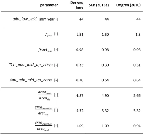
Table 2. Comparison of numerical data derived from the analysis here, the RFI response (SKB, 2015a) and the original RNT model data description (Löfgren, 2010).

parameter Derived

here SKB (2015a) Löfgren (2010)

_ _

adv low mid [mm year-1_] ₄₄ ₄₄ ₄₄

flood

f [-] _1.51 _1.50 _1.3

mire

fract [-] 0.98 0.98 0.98

_ _ _ _

Ter adv mid up norm [-] 0.33 0.30 0.31

_ _ _ _

Aqu adv mid up norm [-] 0.70 0.64 0.64

catch obj area area [-] 4.87 4.90 5.66 watershed obj area area [-] 5.32 5.32 5.32 watershed catch area area [-] 1.09 1.09 0.94

(23)

configuration of the object and catchment during the evolution of the basin. Again, the reliability of the approach taken by SKB is to be questioned. The numerical im-plications are investigated in Section 3, below.

Overall the description of the translation from the details of the MIKE-SHE model-ling via the “average object” to the RNT model has suffered from a lack of attention to detail during the modelling stage and a lack of adequate documentation in the main reports. The RFI has not remedied this. Nevertheless there is reasonable con-vergence between the numerical values derived in different ways. The main caveat is that the parameterisation, with these numerical values, is only suitable for a basin with catch 5 obj area area  .

2.4. Discussion

The Reference Biospheres Methodology (IAEA, 2003) sets guidelines for the defini-tion of models fit for the purposes set out in the regulatory and site contexts. Key steps in the process are “system identification and justification”.

SKB’s definition of the SR-Site radionuclide transport model (an essential compo-nent in the dose assessment modelling) uses MIKE-SHE to characterise water flows in the surface system – this identifies water fluxes in the biosphere system. Moreo-ver, use of MIKE-SHE, linked to detailed site descriptive modelling, provides a quantitative description. It is impractical to use MIKE-SHE directly in the RNT modelling. Instead the results are interpreted to fit the RNT model. The translation of the conceptual understanding provided by MIKE-SHE into the structure of the RNT model therefore requires detailed justification.

There is no justification for the structure of the RNT model in any of the SR-Site documentation, including the response to the RFI. The documentation implies that the RNT model was identified independently of the MIKE-SHE modelling, with only a superficial description of how the flow system for the “average object” was used to populate the database for the RNT model. The structures of the two versions of water fluxes are rather different (Figure 1 and Figure 2) and it is difficult to rec-oncile them (Section 2.2, above).

One area of concern is that the RNT model simplifies exchanges between compart-ments in terms of a net flux. This means that there is a net upwards flux of water in, for example, the exchange between the lower and mid-regolith compartments of the terrestrial sub-system (43 mm year-1_{). However, there is flux of 60 mm year}-1_{with a}

return of 17 mm year-1_{. The net flow of water is the same but the mixing of}

contami-nants may not be adequately represented in by a single net flux, with potential errors if compartmental kds differ significantly..

While the use of net fluxes is understandable in the translation of Figure 1 into Fig-ure 2 the same approach is not used to characterise the flows involving the mid-reg-olith. The numerical value for the flux from TerMid to TerUp cannot be understood. It is quoted as a combination of some (but not all) fluxes into and out of the terres-trial regolith of the “average object”. It is clearly not a “net flux” from the mid-regolith to anywhere else and the justification for combining fluxes in this way is not stated in the available documentation. Similarly the net flow from the aquatic mid-regolith to the lake is based on a selective net flux involving exchanges between the

(24)

terrestrial and aquatic mid-regolith compartments of the MIKE-SHE model, despite the fact that there is no exchange between these compartments in the RNT model. Analysis in Section 2.2 suggests that SKB dissociate the lateral flows in the three- layer “average object”. This would explain why interaction with the lower regolith is not included in the definition of the upwards fluxes in the mid-regolith. The mid- and upper regolith parts of the terrestrial and aquatic subsystems are then combined (according to obscure rules) in the definition of parameters relating to the fluxes be-tween the terrestrial upper and lake water compartments of the RNT model as well as losses from the entire system by drainage.

For these reasons it is clear that the RNT model is not sufficiently well justified. The implications for the transport and accumulation of the differences between the “av-erage object” and the RNT model are further considered in Section 3 below. The generalisation of the fluxes in the RNT model is an essential step in defining a model that can be applied to other basins in the landscape. (Kłos, 2015a has com-mented on the suitability of that feature of the SR-site dose assessment modelling.) As with the interpretation of the “average object” flow system, the way in which this was done lacks transparency.

There is no justification for the parameterisation quoted here in Table 1 (reproduced from SKB, 2015a); the expressions are simply stated. As noted above, there seems to be a distinction between the flow system in the lower and the mid-upper regolith. In the lower regolith the fluxes are represented by a simple advective flux, so that the volumetric water flux out of the lower regolith is adv low mid A_ _ * obj m3 year-1

where, implicitly, the volumetric flux scales with the area of the object and are inde-pendent of the size of the catchment.

Water fluxes associated with the mid-regolith use the normalised runoff to deter-mine the advective fluxes in terms of the total water captured by the basin, for exam-ple the upwards volumetric flux from the terrestrial mid-regolith to the upper rego-lith is Ter adv mid up norm area_ _ _ _ * catch*runoff m3 year.

Flow in the lower regolith is therefore treated differently from flow in the mid and upper regolith. Kłos et al. (2014) have already noted the “snapshot” nature of the model imposed (without discussion) by SKB, in that the areas of the catchment and object are fixed for all stages of the evolution to be representative of the “average object” at 5000 CE, the time at which flows in the “average object” are defined. The differences expressed in Table 2 between the numerical values used to define the RNT model parameters further illustrate the lack of transparency in the definition of the RNT.

The following section of this reports investigates the implications for the concentra-tion of radionuclides in the RNT model.

(25)

3. Numerical implications

3.1. Alternative model for lake-mire

Kłos (2015a) has defined an alternative, evolving basin-scale transport model as part of a dose assessment model that has been used to compare results from SR-Site (Kłos, et al., 2015). That model looked, in part, at alternative interpretations of the overall flow system of the regolith in the whole basin. Results indicate that doses (specifically Landscape Dose Factors – LDFs) calculated by SKB were reasonable and that there were no obvious discrepancies that would lead to higher conse-quences. Overall the uncertainty in results calculated by Kłos et al. (2015a) was bet-ter quantified and more closely linked to the features, events and processes (FEPs) in the basin.

The radionuclide transport model (the RNT model, below) described by Avila et al. (2010) is an approximation of the flow system of the “average object”. It is a set of algebraic relations that are intended to represent a range of potential objects in the landscape. The flow system in the “average object” can be used directly to form a radionuclide transport model that exactly represents transport and accumulation in the “average object” - this is referred to as the AVO RNT model. It is therefore pos-sible to compare the distribution of radionuclides in each of the two models of the “average object”. This comparison illustrates how representative is the Avila et al. RNT model.

Furthermore, the flux maps for the specific lakes used to define the “average object” (see Appendix 2) can also be used to form specific RNT models (based on the AVO RNT model but with modified fluxes). The Avila et al. RNT can be used to model these (since the RNT is designed to represent a wide range of objects). Comparisons of results from the object specific AVO RNT model with the RNT model indicate how well the Avila approach matches the distribution of radionuclides using the ex-act flow systems shown in Appendix 2.

3.2. Model definition

3.2.1. Dataset and structures

The models applied here are non-evolving radionuclide transport models of the lake mire system. All model data and parameters are kept constant, only the radionuclide inventories in the model compartments change in time. The source term for radionu-clides is assumed to be 1 Bq year-1_{of each of}79_Se,94_Nb,129_{I and}226_{Ra (with}

in-growth of daughters 210_{Pb and}210_{Po). The models are run to equilibrium, usually}

(26)

Modified “average object” transport model –

The AVO RNT model, exact implementation of

numerical fluxes for specific objects.

Fluxes in the Avila et al. (2010) radionuclide transport model – The AVO model, an algebraic

simplification of the “average object” flow net-work.

Figure 4. Model structures for the numerical comparison of radionuclide transport and accumulation. These model structures are implemented in Ecolego to simulate radionu-clide transport and accumulation. They are based on the structures shown in Figure 1 (for the “average object”) and Figure 2 (RNT model), but are modified to include common compartments (upper regolith in each model). This requires reinterpretation of the “aver-age object” TerWat compartment as TerUp. See text for details.

Figure 5. Summary of water fluxes (mm year-1_{) in the modified “average object” transport}

model. Modified from Kłos et al. (2015b) to include the additional compartments for the transport modelling. Fluxes from geosphere are inferred from the discussion in Bosson

et al. (2010). Rounding errors in the “average object” mean that perfect balance is not achieved. The yellow compartments define the release distribution. In this case 0.7 and 0.3 Bq year-1_{enter terrestrial and aquatic sub-models respectively.}

TerLow TerMid AquLow AquUp AquMid TerUp AquWat RegoLow TerUp AquUp Aqu_water TerMid AquMid

geosphere catchment TerLow TerMid TerUp AquLow AquMid AquUp AquWat Atm

Down- stream geosphere 7 3 catchment 40 263 497 TerLow 60.0 4.0 6 TerMid 17.0 239.0 492.0 17 TerUp 436.0 791.0 972 AquLow 6.0 9.0 AquMid 10.0 8.0 627.0 AquUp 145.0 627.0 Aqu_ Water 1356.0 145.0 Atm 110 88 Upstream Inflow 0.0 0.0 70.0 769.0 2202.0 15.0 646.0 772.0 1506.0 0.0 995.0 Outflow 10.0 800.0 70.0 765.0 2199.0 15.0 645.0 772.0 1501.0 198.0 0.0 Balance -10.0 -800.0 0.0 4.0 3.0 0.0 1.0 0.0 5.0 -198.0 995.0

(27)

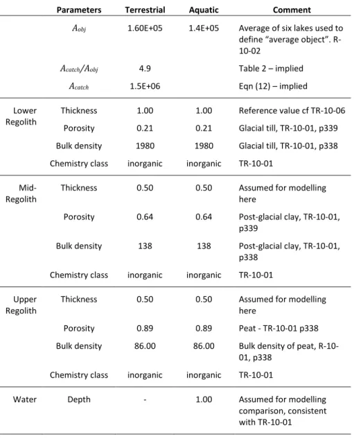
Table 3. Numerical parameters for the model intercomparison. For simplicity all proper-ties of terrestrial and aquatic regolith are assumed to be the same.

Parameters Terrestrial Aquatic Comment

Aobj 1.60E+05 1.4E+05 Average of six lakes used to

define “average object”. R-10-02

Acatch/Aobj 4.9 Table 2 – implied

Acatch 1.5E+06 Eqn (12) – implied Lower

Regolith

Thickness 1.00 1.00 Reference value cf TR-10-06

Porosity 0.21 0.21 Glacial till, TR-10-01, p339

Bulk density 1980 1980 Glacial till, TR-10-01, p338

Chemistry class inorganic inorganic TR-10-01

Mid-Regolith

Thickness 0.50 0.50 Assumed for modelling

here

Porosity 0.64 0.64 Post-glacial clay, TR-10-01,

p339

Bulk density 138 138 Post-glacial clay, TR-10-01,

p338

Upper Regolith

Thickness 0.50 0.50 Assumed for modelling

here

Porosity 0.89 0.89 Peat - TR-10-01 p338

Bulk density 86.00 86.00 Bulk density of peat,

R-10-01, p338

Water Depth - 1.00 Assumed for modelling

comparison, consistent with TR-10-01

R-10-02 – Bosson et al. (2010) TR-10-01 – Löfgren (2010) TR-10-06 – Avila et al. (2010)

Figures quoted are bulk density, 𝜌𝐵. Equivalent grain density, 𝜌, is given by 𝜌𝐵= (1 − 𝜀)𝜌. This uses the

(28)

The RNT model can be used directly with the fluxes as described by Avila et al. (2010), SKB (2015a). However, because the MIKE-SHE generated “average object” does not have upper regolith compartments some reinterpretation is required to for-mulate the AVO RNT model, see Figure 4. A similar approach is taken as with the RNT model interpretation: the aquatic upper regolith compartment is placed be-tween the mid and water (lake) compartments. Fluxes exchanged bebe-tween AquMid and AquWat are assumed to go via AquUp. AquUp is assumed not to be in contact with the terrestrial upper regolith (TerUp) since it represents the bed sediment of the lake.

The TerUp compartment takes the place of the TerWat compartment in the “average object” scheme. The justification for this is that the upper regolith of the mire repre-sents saturated high porosity, loosely consolidated peat (porosity is typically 89%, density is 86 kg m-3_{; Löfgren, 2010). Naturally this changes in time as the system}

matures. For present purposes, then, TerWat ≡ TerUp is reasonable, and the solid content of the compartment is significantly higher than the AquWat compartment. Thickness of the peat layer varies in the landscape (Lindborg, 2015). For reference, we take a compartment thickness of 0.5 m for the upper and mid-regolith layers. The thickness of the lower regolith is assumed to be 1 m in each of aquatic and terrestrial sub-systems. The aquatic compartments have similar properties, the difference being that there is a water column, the depth of which is taken to be 0.5 m. The mid- and lower regolith layers are assumed to be glacial clay (mid-regolith) and till (lower regolith). Radionuclide kds in these media are therefore distinguished as either

or-ganic (peat layers) or inoror-ganic (clay, till). The data are collected in Table 3. The areas of mire and lake are averages of the areas of the six lakes used to define the “average object”, namely A = 1.6E5 mter

2_and

aqu

A = 1.4E5 m2_{.The area of the}

catchment is derived from the total object area using the estimated ratio of catch-ment to object in Table 2.

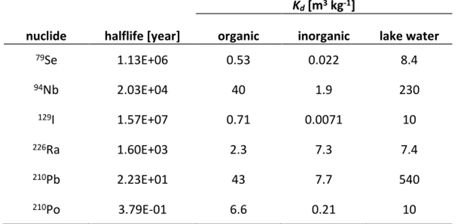
Table 4. Radionuclide specific parameters for the model comparison. Data taken from Nordén et al. (2010). (Kd for lakes ecosystems also included, though not used.)

Kd [m3 kg-1]

nuclide halflife [year] organic inorganic lake water

79_Se _1.13E+06 _0.53 _0.022 _8.4 94_Nb _2.03E+04 ₄₀ _1.9 ₂₃₀ 129_I _1.57E+07 _0.71 _0.0071 ₁₀ 226_Ra _1.60E+03 _2.3 _7.3 _7.4 210_Pb _2.23E+01 ₄₃ _7.7 ₅₄₀ 210_Po _3.79E-01 _6.6 _0.21 ₁₀

(29)

3.2.2. Transfer coefficients

The models here deal only in advective transport. The first order transfer coeffi-cients are written in terms of the water flux from compartment i to compartment j,

ij

F m3_y-1_{and the volume of the donor compartment – the product of thickness, (}

i l m) and surface area (A m_i 2_):



11



ij obj ij i i i i i i F A k l A        year -1_. ₍₁₉₎

This expression uses the compartment’s volumetric moisture content, _i . As all compartments in the model here are saturated, the numerical values are equal to that of the porosity, _i . The radionuclides’ compartmental kds are denoted by k and i the grain density is _i. Numerical values for the radionuclides are listed in Table 4. The factor A_obj m2_{comes from the normalising area used to define the advective}

fluxes in Figure 1. It is clear from Sections 3 and 4 of SKB (2015a) that this is the total area of the object, A_objA_TerA_Aqu (cf. the parametrisation in Table 1). The numerical values of the fluxes discussed in Section 2.2 above must effectively be transformed to as volumetric fluxes:

AVO RNT model: mm year-1 m year3 -1

1000

ij obj ij

F A

F _ _ _ _ year-1_,

RNT model: mm year-1 m year3 -1

1000 ij obj ij A       _ _ _ _ year-1_.

3.3. Results

3.3.1. Overview of calculations

The questions addressed in this section of the report are:

i. Is the RNT model an adequate representation of the “average object” flow sys-tem?

ii. How does the RNT interpretation compare to results using the individual flow systems generated by MIKE-SHE and on which the “average object” is based? This analysis does not consider whether the use of the RNT model is right or wrong, rather the intention is to examine how representative is the simplified model com-pared to the implementation of the exact fluxes. In this way this report provides the justification step that SKB have not addressed adequately. The analysis indicates the degree of confidence that the reviewer can have in the original Avila et al. (2010) RNT model. There are two stages:

i. Comparison of results from the modified AVO RNT model with those from the RNT model using the fluxes discussed in Section 2.2 for the “average object”

(30)

ii. Comparison of the parameterised RNT model as applied to selected lakes that SKB used to generate the “average object”, using the numerical fluxes provided in response to request 2 of the original RFI (see Appendix 1).

As the models run non-evolving system the aim is to compare the distribution of ra-dionuclides in the system over a period of 105_{years to illustrate the implications of}

the two flow system interpretations. Of primary interest is the accumulation of radi-onuclides in the terrestrial upper regolith (TerUp) and the aquatic water column (AquWat) since it is from these two compartments that doses would be derived. The TerUp compartment is used in Avila et al. (2010) to define the initial concentration in agricultural soils following conversion from their natural state (as modelled using the RNT model here).

As well as the time series for compartmental inventories that are produced in the Ecolego implementation of the two models, the ratio of inventories is used as a guide to similarity; for the ith_{compartment in the RNT model (the inventories in the}

terrestrial and aquatic lower regolith compartments of the AVO RNT model are summed to correspond to the single lower regolith compartment of the RNT model). The ratio is then







i



i i N RNT r N AVORNT  . (19)

for i = Low, AquMid, AquUp, TerMid, TerUp, AquWat, Sink.

With the exception of the sink inventory, r_i1 means that the SKB model is con-servative. For the sink compartment the opposite is true since r_sink1 means that more activity is retained in the RNT compartments than in the AVO RNT model.

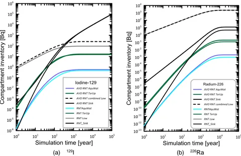
(a) 129_I _(b) 226_Ra

Figure 6.Comparison of selected inventories for 129_{I (weakly sorbing) and}226_{Ra (strongly}

(31)

3.3.2. Model of the “average object” flow system.

At first sight (Figure 6), the agreement between the AquWat, TerUp and Low and Sink compartment inventories appears to be good. For 129_{I, with relatively weak}

sorption, the biggest difference is seen between the lower regolith content. This is influenced by the two distinct lower regolith compartments in the AVO RNT model. At earlier times the loss from the system slightly greater but this is resolved beyond a few hundred years, when equilibrium in the system is established. For 226_{Ra the}

lower regolith content is identical – a function of retention – but there are clear, though small, differences in the water and upper regolith compartments. The AVO RNT model loses a greater quantity of activity downstream.

The surprise is not that there are some differences, it is that the results are so similar given the differences in the model structures seen in Figure 4. The plots of the in-ventory ratios in Figure 7 help to explain these results.

The six radionuclides shown in Figure 7 illustrate the role played by sorption and in-growth. With relatively low kds both 79Se and 129I show similar responses. For the

more strongly sorbing 94_{Nb and}226_{Ra there are again similarities.}210_{Pb and}210_Po

grow from the released 226_{Ra. They too have relatively high sorption. Results for}

these three members of the 226_{Ra decay chain are broadly similar and secular}

equi-librium is established fairly rapidly.

Overall these results support what was seen in Figure 6, namely that the AVO RNT and RNT models are in reasonable agreement. The value of r = 1 is shown and the _i lower kd nuclides are close to this throughout, sometimes higher (RNT is

conserva-tive) sometimes lower. For the higher kd nuclides the RNT is always

non-conserva-tive for TerUp inventories but the effect is small. In fact the RNT model is always non-conservative for the more sorbing species (except for AquWat at earlier times). Nevertheless it might be concluded that the RNT model is a practical representation of the flow system. The result for the TerMid compartment for 79_{Se and}129_{I suggests}

further investigation, however. Although not a high ratio (≈ 2) it is necessary to ex-plain what is happening, especially as the flow systems appear so different in Figure 4.

The TerUp agreement is generally good, more so for low than high kd. An analysis

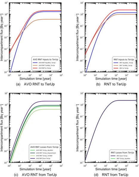
of the radionuclide fluxes into and out of the TerUp compartments of the two mod-els is shown in Figure 8 for 129_{I and Figure 9 for}226_Ra.

The total input to of 129_{I to TerUp is similar in each model (red line in Figure 8 a and}

b). However, how this total input is derived is different in each model. The release is predominantly to the terrestrial side and so, at earlier times, input is via the terres-trial mid regolith. For the first ten years this route dominates. Thereafter transfers via the aquatic system take over. The transition is earlier for the AVO RNT model and the final flux from TerMid is significantly lower than in the case of the RNT model. Similarly the equilibrium value of the transfer from AquWat is higher than in the case of the RNT model.

Although the overall input to the upper terrestrial regolith is close in the two models over the period of the simulation, the input via TerMid is of greater importance in the RNT model. In part this relative importance of TerMid in the RNT model stems from the accumulation in this compartment in the ratios plot, Figure 7c.

(32)

(a) 79_Se _(b) 94_Nb

(c) 129_I _(d) 226_Ra

(e) 210_Pb _(f) 210_Po

Figure 7. Ratios of compartment inventories – RNT model : AVO RNT model. Results for all six radionuclides in the modelled system. Agreement between the models is denoted by the dashed line at r = 1.

(33)

For 129_{I here, flow from the lower regolith of the AVO RNT is of lesser importance.}

Loss from TerUp is to water in the RNT and this corresponds to the sum of all losses from in the AVO. Losses from TerUp are controlled by a single flux in the RNT model and this corresponds closely to the combined fluxes to TerMid, AquWat and Downstream. This is easier to understand. Results for 79_{Se, also with a low k}

d, are

similar.

In the case of 226_{Ra (higher k}

d radionuclide) there is a greater discrepancy between

the total flux into TerUp, as seen in the red lines of Figure 9a & b. The difference is less than a factor of two and, as with 129_{I, the main source of}226_{Ra into the upper}

regolith in the AVO RNT model is from the water compartment. Fluxes from the water compartment in the RNT model are lower. Both models give a similar flux from TerMid to TerUp.

(a) AVO RNT to TerUp (b) RNT to TerUp

(c) AVO RNT from TerUp (d) RNT from TerUp

(34)

In the case of 226_{Ra (and the other higher k}

d radionuclides) the overall content of the

terrestrial upper compartment is lower because there is a lower input from AquWat. In turn, this is a consequence of the lower inventory in the water compartment (cf. Figure 7d for 226_{Ra and b, e and f for the other strong sorbers. As seen for}129_{I, input}

to the terrestrial sub-system dominates at earlier times and the transfer from TerMid to TerUp dominates for the first 100 years. The effect of kd is to smooth out the

dif-ferences between the models and the earlier development of fluxes into TerMid is similar over the first 1000 years.

Taking the inventory in TerUp as a benchmark, results for the “average object” (used to calibrate the RNT model) suggest that the RNT model works reasonably well; for weakly sorbing species because there is little retention in the system and thereby a higher loss from the water column, activity reaches TerUp via the TerMid

(a) AVO RNT to TerUp (b) RNT to TerUp

(c) AVO RNT from TerUp (d) RNT from TerUp