BACHELOR THESIS IN
AERONAUTICAL ENGINEERING
15 CREDITS, BASIC LEVEL 300
Modelling & implementation of
Aerodynamic Zero-lift Drag into
ADAPDT
Author: David Bergman
Report code: MDH.IDT.FLYG.0215.2009.GN300.15HP.Ae
TDAA-EXB, David Bergman 2009-11-03 1 1 (46)
Fastställd av Confirmed by Infoklass Info. class Arkiveringsdata File
TDAA-RL, Roger Larsson PUBLIC TDA-ARKIV
Giltigt för Valid for
T h is d o cu m e n t a n d t h e i n fo rm a tio n co n ta ine d h e re in is th e p ro p e rty o f S a a b A B a n d m u st n o t b e u se d , d iscl o se d o r a lte re d with o u t S a a b A B p rior w ritte n co n se n t.
Ärende Subject Fördelning To
Modelling & implementation of Aerodynamic Zero-lift Drag into ADAPDT
TDAA-RL, TDAA-PW, TDAA-SH, TDAA-ET, TDAA-HJ,
Gustaf Enebog (MDH) ABSTRACT
The objective of this thesis work was to construct and implement an algorithm into the program ADAPDT to calculate the zero-lift drag profile for defined aircraft geometries. ADAPDT, short for AeroDynamic Analysis and Preliminary Design Tool, is a program that calculates forces and moments about a flat plate geometry based on potential flow theory. Zero-lift drag will be calculated by means of different hand-book methods found suitable for the objective and applicable to the geometry definition that ADAPDT utilizes.
Drag has two main sources of origin: friction and pressure distribution, all drag acting on the aircraft can be traced back to one of these two physical phenomena. In aviation drag is divided into induced drag that depends on the lift produced and zero-lift drag that depends on the geometry of the aircraft.
How reliable and accurate the zero-lift drag computations are depends on the geometry data that can be extracted and used. ADAPDT‟s geometry definition is limited to flat plate geometries however although simple it has the potential to provide a huge amount of data and also deliver good results for the intended use. The flat plate representation of the geometry proved to be least sufficient for the body while wing elements could be described with much more accuracy. Different empirical hand-book methods were used to create the zero-lift drag algorithm. When choosing equations and formulas, great care had to be taken as to what input was required so that ADAPDT could provide the corresponding output. At the same time the equations should not be so basic that level of accuracy would be compromised beyond what should be expected from the intended use.
Finally, four well known aircraft configurations, with available zero-lift drag data, were modeled with ADAPDT‟s flat plate geometry in order to validate, verify and evaluate the zero-lift drag algorithm‟s magnitude of reliability. The results for conventional aircraft geometries provided a relative error within 0-15 % of the reference data given in the speed range of zero to Mach 1.2. While for an aircraft with more complicated body geometry the error could go up to 40 % in the same speed regime. But even though the limited geometry is grounds for
uncertainties the final product provides ADAPDT with very good zero-lift drag estimation capability earlier not available. A capability that overtime as ADAPDT continues to evolve has the potential to further develop in terms of improved accuracy.
Date: October 25, 2009
Carried out at: Saab Aerosystems, Linköping, Sweden Advisor at MDH: Gustaf Enebog
Advisor at Saab Aerosystems: Roger Larsson Examinator: Gustaf Enebog
T h is d o cu m e n t a n d t h e i n fo rm a tio n co n ta ine d h e re in is th e p ro p e rty o f S a a b A B a n d m u st n o t b e u se d , d iscl o se d o r a lte re d with o u t S a a b A B p rior w ritte n co n se n t. SAMMANFATTNING
Målet med detta examensarbete var att skapa och implementera en algoritm som inför möjligheten att beräkna nollmotstånd för givna flygplansgeometrier i programmet ADAPDT. ADAPDT, kort för AeroDynamic Analysis and Preliminary Design Tool, är ett program som, baserat på potential strömnings teori, beräknar krafter och moment på en geometri uppbyggd av plana plattor. Nollmotståndet kommer att baseras en kombination av handboksmetoder som funnits lämpliga och applicerbara på geometridefinitionen given i ADAPDT.
Motstånd har sitt ursprung i två fysikaliska fenomen: friktion och tryckfördelning, ur vilka allt motstånd som agerar på ett flygplan härrör. Inom flyget delar man in motståndet i
lyftkraftsberoende inducerat motstånd samt geometriberoende nollmotstånd.
Hur pålitliga och noggranna motståndsberäkningarna kan förväntas vara beror på mängden geometriska data som finns att tillgå. ADAPDT:s geometridefinition är begränsad till plana plattor men trots detta finns potential att leverera stora mängder data och resultat med rimlig noggrannhet. Plan plattgeometrin visade sig, för kroppsgeometrin, väldigt begränsad och otillräcklig medan ving element kunde beskrivas med större noggrannhet.
En rad olika empiriska handboksmetoder användes för att skapa nollmotståndsalgoritmen. Vid valet av formler och ekvationer var det viktigt att välja sådana som ADAPDT kunde förse tillräckligt med data till. Samtidigt fick formlerna inte vara alltför simpla så att måttet av noggrannhet i resultaten vart alltför låg mot för vad som, för ändamålet, är förväntat. Slutligen valdes fyra kända flygplan, med nollmotståndsdata tillgängligt, att modeleras med ADAPDT:s plan plattgeometri för att validera, verifiera och utvärdera algoritmens mått av tillförlitlighet. Resultaten för mer konventionella flygplanskonfigurationer visade på ett relativt fel mellan 0-15 % mot de givna referensflygplanens nollmotståndsdata inom hastigheterna 0 till Mach 1,2. För mer komplicerade konfigurationer steg det relativa felet omedelbart upp mot 40 % inom samma hastighetsregim. Men även om den begränsade geometridefinitionen i
ADAPDT är grunden för mycket osäkerheter förser den slutliga produkten ändå programmet med en väldigt god möjlighet till skattning av nollmotståndet som inte tidigare fanns. En möjlighet som över tid, allteftersom ADAPDT forstätter att utvecklas, har all potential till att förbättras med avseende på noggrannhet och tillförlitlighet.
T h is d o cu m e n t a n d t h e i n fo rm a tio n co n ta ine d h e re in is th e p ro p e rty o f S a a b A B a n d m u st n o t b e u se d , d iscl o se d o r a lte re d with o u t S a a b A B p rior w ritte n co n se n t. ACKNOWLEDGEMENTS
Foremost I would like to thank my supervisor and mentor Roger Larsson at Saab Aerosystems for giving me the opportunity to do this Bachelor‟s thesis work at Saab. The help and support you provided always gave me a big push forward with my work. Also thanks for letting me play floor ball with you and for all the great laughs and fun moments.
Huge thanks to my examiner Gustaf Enebog at Mälardalen University for providing very comprehensive feedback on my report and help during the final stages of my thesis project. I would also like to acknowledge Svante Hellzen and Ernst Totland. Svante, thanks for showing great interest in my work with your GUI and for all the help and feedback you gave me. Ernst, thanks for sharing your great knowledge and expertise of drag calculations with me. The feedback and help you gave me always pointed me in the right direction and when possible you provided me with good documents where I could find what I searched for by myself.
I want to dedicate special thanks to Nina Hagberg and Johan Hammar who had their working spaces in front of and behind me. It was a pleasure to be able to chit chat with you and to share many extremely fun moments and great laughs in the office space and of course also outside of the office space.
Finally I want to thank everyone that I haven‟t mentioned but who also supported me during my time at Saab and came to listen to my presentation.
T h is d o cu m e n t a n d t h e i n fo rm a tio n co n ta ine d h e re in is th e p ro p e rty o f S a a b A B a n d m u st n o t b e u se d , d iscl o se d o r a lte re d with o u t S a a b A B p rior w ritte n co n se n t.
NOTATIONS
A AreaAbase Base area
Aextra Extra area not covered by side or top view
Amax Maximum cross-sectional area
Aroot Root area
Aside Side-view area of the aircraft
Atop Top-view area of the aircraft
Awet Wetted area
AwR
Body wetted area corrected for wings, fins, stabilizers and other attachments that reduce the body wetted area
ADAPDT AeroDynamic Analysis and Preliminary Design Tool
b Wing span
br Body radius
c Chord
CD Coefficient of drag
CD0 Zero-lift drag coefficient
CDb Base drag coefficient
CDcreep
Drag rise between the critical mach number and the drag divergence mach number
CDF Friction drag coefficient
CDint Interference drag coefficient
CDi Induced drag coefficient
CD,M=1,2 Coefficient of drag at Mach 1,2
CD,MDD Coefficient of drag at the drag divergence mach number
CDMisc Drag coefficient due to miscellaneous factors added
CDP Pressure drag coefficient
CDW Wave drag coefficient
Cl Lift coefficient
CP Pressure coefficient
CR Root Chord
CT Tip Chord
D Diameter
EWD Empirical wave drag efficiency factor
e Oswald efficiency factor
gui Graphical User Interface
H Enthalpy
k Integral core
L Airfoil thickness location parameter
l Length
T h is d o cu m e n t a n d t h e i n fo rm a tio n co n ta ine d h e re in is th e p ro p e rty o f S a a b A B a n d m u st n o t b e u se d , d iscl o se d o r a lte re d with o u t S a a b A B p rior w ritte n co n se n t.
MDD Drag divergence mach number
p Pressure
R Reynolds number per meter
RLS Sweep angle correction factor
r Radius
S Entropy
Sref Reference area
Vbody Body volume
Vtot Total volume
xt Length wise position along chord
α Angle between free stream and aircraft x-axis (angle-of-attack)
α 0
Angle between the aircraft x-axis and the wing‟s zero-lift alpha angle
Γ Ring vortex strength
γ Constant set to 1,4 for air
ΔClb
Coefficient factor to interference drag depending upon if the wings, fins, stabilizers or canards are place high, mid or low on the aircraft
ΔM Difference between critical mach number and drag divergence
mach number
Λc/4 Quarter chord sweep angle
ΛLE-deg Leading edge sweep angle in degrees
λ Root-tip chord ratio (taper ratio)
μ Unknown function
ρ Density
φ Interference potential
Ω Wake behind aircraft
V
Velocity Vector
Free stream potentiali Panel coordinate system i direction
j Panel coordinate system j direction
(D/q)Sears-Haack Coefficient of wave drag according to Sears-Haack formula
t/c Thickness to chord ratio
x Global x-axis
y Global y-axis
T h is d o cu m e n t a n d t h e i n fo rm a tio n co n ta ine d h e re in is th e p ro p e rty o f S a a b A B a n d m u st n o t b e u se d , d iscl o se d o r a lte re d with o u t S a a b A B p rior w ritte n co n se n t. TABLE OF CONTENT ABSTRACT ... 1 SAMMANFATTNING ... 2 ACKNOWLEDGEMENTS ... 3 NOTATIONS ... 4 1 INTRODUCTION ... 7 1.1 BACKGROUND ... 7 1.2 REPORT STRUCTURE ... 7
2 INTRODUCING DRAG & THE ADAPDT PROGRAM ... 8
2.1 DRAG ... 8
2.1.1 Induced drag ... 10
2.1.2 Skin Friction Drag ... 10
2.1.3 Pressure Drag ... 11 2.1.4 Interference Drag ... 12 2.1.5 Base Drag ... 12 2.1.6 Wave Drag ... 13 2.2 ADAPDT... 14 2.2.1 Background ... 14 2.2.2 Interface ... 14 2.2.3 Working ADAPDT ... 15 3 THEORY ... 18 3.1 DRAG MODELING ... 18 3.1.1 Subsonic Drag ... 19 3.1.1.1 Wing areas ...19 3.1.1.2 Bodies ...21
3.1.1.3 Horizontal Stabilizer or Canard ...22
3.1.1.4 Fin ...22 3.1.1.5 Roughness/Cooling ...23 3.1.2 Transonic Drag-rise ... 23 3.1.3 Supersonic Drag ... 25 3.2 ADAPDTMATHEMATICS ... 26 3.2.1 Linear... 26 3.2.2 Nonlinear ... 27 4 RESULTS ... 28 4.1 THE ALGORITHM ... 28 4.2 IMPLEMENTATIONS ... 29
4.2.1 Define Faces tool ... 29
4.2.2 Plot Zero-lift Drag tool ... 31
4.2.3 Add profile camber and thickness tool ... 32
4.3 VALIDATION AND VERIFICATION ... 33
4.3.1 Boeing 727-100 ... 33
4.3.2 F-4e Phantom ... 34
4.3.3 T-38 Talon ... 35
4.3.4 F-104G Starfighter ... 36
5 DISCUSSION & CONCLUSION ... 37
5.1 THE ALGORITHM ... 37
5.2 DRAG CALCULATIONS ... 37
5.3 VALIDATION AND VERIFICATION ... 38
6 RECOMMENDATIONS ... 39
7 REFERENCES ... 40
T h is d o cu m e n t a n d t h e i n fo rm a tio n co n ta ine d h e re in is th e p ro p e rty o f S a a b A B a n d m u st n o t b e u se d , d iscl o se d o r a lte re d with o u t S a a b A B p rior w ritte n co n se n t. 1 INTRODUCTION
This paper presents the results of a Bachelor‟s degree thesis work at Mälardalen University, Västerås, Sweden. It is the last part of the authors three year education which, when finished, will grant him a Bachelor‟s degree in aeronautical engineering.
The work was carried out at the Aerodynamics and Flight Mechanics Department at Saab Aerosystems, Linköping, Sweden.
1.1 Background
When working with design and concept studies it is imperative to have a simple program that can deliver good and reasonable results within a short amount of time. The short time is especially in focus since a large number of configurations and cases are to be simulated. ADAPDT is such a conceptual design however it lacks the ability to estimate zero-lift drag. The objective of this work is to construct an algorithm that can calculate, plot and give a reasonably good indication of what zero-lift drag profile to expect for a configuration. Calculations will be based on the geometry definition ADAPDT utilizes and by means of different hand-book methods suitable for computer implementation.
When the algorithm has been created it is to be validated and verified by running known aircraft configurations through the program and comparing the results with the configuration‟s
reference data. Finally the algorithm will be implemented into ADAPDT to be a part of the program for future concept studies at Saab Aerosystems.
1.2 Report Structure
This report is divided into 5 major chapters that will take the reader through the entire work. By reading the report top down the reader is expected to grasp what the work is about, the problems encountered and finally understand the results obtained.
The first and current chapter starts out by giving the reader a quick welcome to this paper, briefly explaining the objective of the work that is done and described within.
Chapter two is designed to give the reader insight into what the work is about by explaining some basic theory about the ADAPDT program and what drag is so that the following chapters may be better understood.
Chapter three introduces the theory to the reader by presenting and explaining all the
mathematical equations used in the drag algorithm. Some brief theory into the potential theory mathematics behind ADAPDT will also be described here.
Chapter four will present the final results of this Bachelor‟s thesis work. Here the reader is taken through how the final algorithm is constructed followed by the implementations that were done into ADAPDT. The chapter concludes by showing four test simulations done with the algorithm and the outcome of them.
The paper concludes with chapter five, in which the writer discusses the work results and presents his conclusions.
T h is d o cu m e n t a n d t h e i n fo rm a tio n co n ta ine d h e re in is th e p ro p e rty o f S a a b A B a n d m u st n o t b e u se d , d iscl o se d o r a lte re d with o u t S a a b A B p rior w ritte n co n se n t.
2 INTRODUCING DRAG & THE ADAPDT PROGRAM
The first part of this section is dedicated to briefly introduce the concept of drag and how it is applied in the aviation industry. The second part will describe how the ADAPDT program works, what it delivers and how it is used. Further mathematical depth into the theory of the program ADAPDT and Drag calculations will be given in chapter 3.
2.1 Drag
Drag is a force generated on an object moving through a fluid, in this case the aircraft moving through air. Overall the forces acting on the aircraft can be simplified into four: lift, thrust, drag and gravity.
Figure 2-1. The four main forces on an aircraft. In aviation drag is divided into two types due to their main source of origin :
Induced Drag (drag due to lift)
Zero-lift Drag (drag due to geometry configuration)
These two differ in the parameters they depend upon but are both related toairspeed. At higher speed the zero-lift drag dominates over the induced drag, while at lower speed it is the opposite as shown by figure 2-2. The point where the two curves intersect indicates airspeed for
optimum aircraft glide performance due to minimum total drag, (L/D)max.
Figure 2-2. Induced -and Form Drag variation with airspeed.
How the total drag changes for different operating conditions is very important to consider due to it having a direct affect on the aircraft‟s efficiency and performance.
T h is d o cu m e n t a n d t h e i n fo rm a tio n co n ta ine d h e re in is th e p ro p e rty o f S a a b A B a n d m u st n o t b e u se d , d iscl o se d o r a lte re d with o u t S a a b A B p rior w ritte n co n se n t.
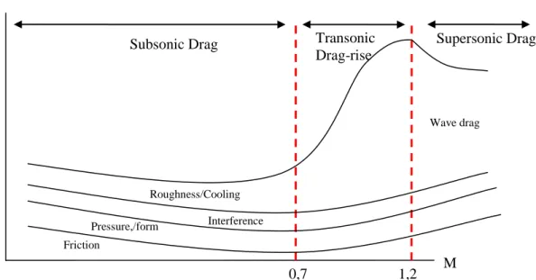
Generally, when estimating zero-lift drag for a configuration, the end objective is to construct a drag curve looking like the one in figure 2-3. The procedure to do this requires that the drag for the subsonic, transonic and supersonic regimes, as outlined by figure 2-3 and depending on the configuration of interest, be calculated. Subsonic drag usually stretches from stand-still to about M=0,7 where the transonic drag-rise starts. The dramatic drag-rise occurs due to locally appearing supersonic flow over different parts the aircraft creating energy stealing shock-waves experienced, by the aircraft, as drag. When the peak of the transonic drag-rise is passed the aircraft has broken through the “sound barrier”. The drag will drop some when entering the supersonic drag regime due to the entire flow over the aircraft now being supersonic. Nowadays, however, it has, in some cases become desirable to make the transonic drag-rise more gradual to eliminate the peak when flying close to supersonic speed. This because the need to operate in supersonic speed has come to be less necessary while the need to be able to operate close to or in the transonic regime has gained more importance. Therefore to minimize the total drag this gradual transition is preferable because it allows the airplane to actually operate in the transonic regime.
Figure 2-3. General outline of conventional zero-lift drag curve.
Zero-lift drag occurs due to two physical phenomena: friction and pressure distribution where almost all forces on the aircraft with friction as origin act as zero-lift drag. These two
phenomena make up the origins of the five different types of zero-lift drag acting on the aircraft:
Origin in friction:
Friction drag Origin in pressure distribution:
Pressure drag (or form drag)
Interference drag
Base drag
Wave drag
Due to the focus of this thesis work being on zero-lift drag the induced drag will be given a very brief introduction first followed by a more thorough explanation of each zero-lift drag listed above. Supersonic Drag Subsonic Drag Transonic Drag-rise 0,7 1,2 CD,0 M
T h is d o cu m e n t a n d t h e i n fo rm a tio n co n ta ine d h e re in is th e p ro p e rty o f S a a b A B a n d m u st n o t b e u se d , d iscl o se d o r a lte re d with o u t S a a b A B p rior w ritte n co n se n t. 2.1.1 Induced drag
The induced drag originates from the difference in air pressure between the top and bottom side of the wing and relies mainly upon the coefficient of lift Cl that the wing produces. The
magnitude of Cl in turn depends upon how large the angle of attack, the alpha angle, is. CDi uses
the formula below:
eAR
C
C
l Di
2
The formula states that the magnitude of the coefficient of induced drag is proportional to Cl
squared and inversely proportional to:
, the oswald efficiency factor e and the wing‟s aspect ratio AR that is described by the equation below:ref
S
b
AR
2
2.1.2 Skin Friction Drag
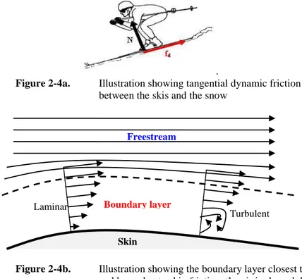
Skin friction drag arises because of the viscosity in the air that flows in the boundary layer closest to the skin of the object. Viscosity is a molecular resistance that fluids exhibit against displacement relative to each other and with respect to the surface of solid objects. This can roughly be compared to the illustration of the skier in figure 2-4a below. When the skier slides on the snow the surface of the ski and snow slide along another and give cause to a tangential force, slowing him down, that is skin friction drag. Similar in aviation when air flows in the boundary layer closest to the skin of the wing, or other area, the air is slowed down to a stand-still closest to the body, figure 2-4b.
.
Figure 2-4a. Illustration showing tangential dynamic friction force acting between the skis and the snow
Figure 2-4b. Illustration showing the boundary layer closest to the skin and how, due to skin friction, the air is slowed down. The magnitude of the skin friction drag is determined mainly by airspeed, wetted area and surface smoothness. The smoother the surface is the more freely air can move over it without being slowed down. But even a rougher surface can produce less friction drag if the airflow is kept laminar over the surface longer.
Freestream
Skin Boundary layer Laminar
T h is d o cu m e n t a n d t h e i n fo rm a tio n co n ta ine d h e re in is th e p ro p e rty o f S a a b A B a n d m u st n o t b e u se d , d iscl o se d o r a lte re d with o u t S a a b A B p rior w ritte n co n se n t.
Laminar flow is when the airflow follows the streamlines over a wing this produces less drag than the turbulent flow that usually occurs as vortexes creating large amount of drag. At wings there is usually a specific point downstream where the transition from laminar to turbulent flow occurs if this transition can be postponed drag could be substantially reduced because of less turbulent flow over the wing. However the laminar flow over the wing is fairly small when compared to the amount of turbulent flow which is why the airflow over the entire wing, in most cases, is considered completely turbulent when dealing with drag estimations.
2.1.3 Pressure Drag
Pressure drag arises because of pressure differentials at different parts of the body figure 2-5a. Unlike skin friction drag, which is a tangential force, pressure drag results from the distribution of forces normal to the surface of the body. One of the main causes to this drag is the separation that occurs in the boundary layer. Air in the boundary layer wants to flow from higher pressure areas to lower pressure areas but if the pressure rises downstream, as shown in figure 2-5b, then the air in the boundary layer will slow down.
Figure 2-5a. Normal pressure distribution over a wing profile.
Figure 2-5b. The rising pressure upstream (upper graph) and the velocity profile change with location S (lower image).
The result is that the continuous airflow will grind to a halt and cause separation. Giving cause to the forming of a wake behind the body adding further to the pressure drag as seen in figure 2-5c. Thus to reduce the pressure drag the body needs to be made as sleek and streamlined as possible to prevent or at least postpone the separation as much as possible.
Lower pressure
T h is d o cu m e n t a n d t h e i n fo rm a tio n co n ta ine d h e re in is th e p ro p e rty o f S a a b A B a n d m u st n o t b e u se d , d iscl o se d o r a lte re d with o u t S a a b A B p rior w ritte n co n se n t.
Figure 2-5c. Different figures showing the pressure drag behind in the wake caused by separation.
2.1.4 Interference Drag
Interference drag is caused by vortices originating from junctions, at sharp concave angles, between parts of an object, for example wing and fuselage as shown by figure 2-6a. These vortices, caused by the acceleration of air due to higher pressure around these parts, give rise to drag. To minimize interference drag all the sharp junctions need to be smoothed out, this is done by adding fillets between the parts, figure 2-6b.
Figure 2-6a. Vortices originating from sharp junctions between wing and body
Figure 2-6b Principal sketch of fillets used to reduce interference drag.
2.1.5 Base Drag
Base drag is formed in the vacuum behind objects with an abruptly cut of end section. Air with higher pressure will flow into the lower pressure region in a turbulent manner, as seen in figure 2-7a, creating drag. To minimize the base drag a boat-tail transition from mid section diameter to trailing edge diameter should be done as gradually as possible, figure 2-7b.
Body Wing
T h is d o cu m e n t a n d t h e i n fo rm a tio n co n ta ine d h e re in is th e p ro p e rty o f S a a b A B a n d m u st n o t b e u se d , d iscl o se d o r a lte re d with o u t S a a b A B p rior w ritte n co n se n t.
Figure 2-7a. The vacuum behind a bullet with abruptly cut of end section as it is fired away. (The surrounding airflow with higher pressure will stream into the lower pressure area in a turbulent manner)
Figure 2-7b. Same bullet as in 2-6a but now with a boat-tail formed end-section. The lower pressure region is smaller than in a resulting in less turbulent airflow behind, reducing drag.
2.1.6 Wave Drag
Wave Drag starts to form when the local airflow around some part of the airplane becomes supersonic, greater than M=1. The airspeed where this occurs is called the Critical Mach Number, Mcrit and is often used to announce the beginning of the transonic speed regime.
Supersonic flow is very different from subsonic because there will always be pressure drag present because of the energy lost due to the forming of shock waves as seen in figure 2-8 below.
Figure 2-8. The X-15 fired into a wind-tunnel show the forming of shock waves
around the airplane at Mach 3,5.
The airplane, that creates these shock waves, experiences the energy loss as pressure drag acting upon the surface of the airplane, counteracting its movement. The pressure force resultant acting in the flight direction is called wave drag.
Bullet D
T h is d o cu m e n t a n d t h e i n fo rm a tio n co n ta ine d h e re in is th e p ro p e rty o f S a a b A B a n d m u st n o t b e u se d , d iscl o se d o r a lte re d with o u t S a a b A B p rior w ritte n co n se n t. 2.2 ADAPDT
ADAPDT, which stands for AeroDynamic Analysis and Preliminary Design Tool, is a program developed by Per Weinerfeldt and Svante Hellzén at Saab Aerosystems Department of
aerodynamics and flight mechanics in Linkoping. The goal is to develop the program to such an extent that it can replace the NASA-developed program Wing-Body, originally created in the 1960‟s, as the primary tool used for preliminary design studies. The program and how it works will be explained in this section. For further information on the mathematical theory see chapter 3.
2.2.1 Background
The lack of a good program that could perform quick calculations on unconventional aircraft geometries was the main reason to start developing ADAPDT. In the early stage of aircraft design it is imperative to be able to quickly predict forces and moments on a large number of configurations. To do this the aircraft geometries are often very simplified and described by flat surfaces which can then be entered into the appropriate software for performance calculations. The results given are expected to be within reasonable boundaries to give an indication of what forces and moments to expect from the current configuration. Saab has since the 1960‟s used the NASA developed linear program Wing-Body (B) to perform these computations. But W-B performs very poorly for unconventional designs such as flat bodies, low aspect ratio wings and bodies with sharp leading edges due to its inability to account for the nonlinearities in the airflow, such as vortices, that occur around these parts. ADAPDT tries to capture these nonlinearities for these unconventional without increasing the computational time.
2.2.2 Interface
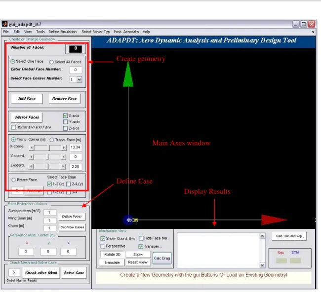
When working with design studies it is imperative to have a simple and well structured interface to work with. A good program should be self explanatory and not take the user that long to get accustomed to. Therefore a GUI that simplified and improved the usage of ADAPDT was constructed. The main window of ADAPDT is shown in figure 2-9 below. It consist of a window where the geometry is built and visualized, the side bars are for creating the geometry, setting flow field values, checking the aircraft mesh and finally running and
T h is d o cu m e n t a n d t h e i n fo rm a tio n co n ta ine d h e re in is th e p ro p e rty o f S a a b A B a n d m u st n o t b e u se d , d iscl o se d o r a lte re d with o u t S a a b A B p rior w ritte n co n se n t.
Figure 2-9. The main workspace in ADAPDT with general sections outlined. The interface also features a number of tools, under development, to use when working, defining and checking simulation results found at the top of the interface as menu bars:
Tools: contains tools to assist with the geometry creation.
Define Simulation: To improve or specify the simulation this bar offers possibilities to further define the simulation to the user‟s preferences.
Select Solver Type: Select which theory the program shall use to solve the problem.
Post Aerodata: In this section the user can choose between different Aero data to be displayed as plots or graphs created by Matlab.
2.2.3 Working ADAPDT
To create a new geometry is simple, choose file, click new case and start building the aircraft by adding and arranging panels. Geometries can also be saved and loaded. For the following example the Gripen geometry, in figure 2-10a and 2-10b, will be loaded and used during this demonstration.
Create geometry
Main Axes window
Define Case
T h is d o cu m e n t a n d t h e i n fo rm a tio n co n ta ine d h e re in is th e p ro p e rty o f S a a b A B a n d m u st n o t b e u se d , d iscl o se d o r a lte re d with o u t S a a b A B p rior w ritte n co n se n t.
Figure 2-10a. JAS 39 Gripen Top down view in ADAPDT Figure 2-10b visualizes very well that the entire geometry only consists of flat surfaces connected to form a simplified limited geometry model.
Figure 2-10b. JAS 39 Gripen front view in ADAPDT
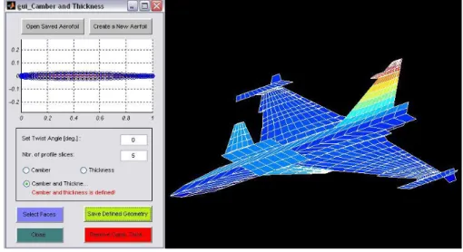
When the geometry is defined a flow case is set, by clicking “Set Flow Cases” which opens up a new interface, figure 2-11. When the flow case is set and saved the next step is to choose a profile for each wing area. To do this scroll down in the “Tools” menu bar and select “Add Profile Camber and Thickness”. Doing this brings up the interface, figure 2-12 left, where profiles can either be loaded or created, leaving only to select which areas the chosen profile is to be imported to giving a result as shown in figure 2-12 right part.
T h is d o cu m e n t a n d t h e i n fo rm a tio n co n ta ine d h e re in is th e p ro p e rty o f S a a b A B a n d m u st n o t b e u se d , d iscl o se d o r a lte re d with o u t S a a b A B p rior w ritte n co n se n t.
Figure 2-12 Interface to select and add a profile to the geometry, here a Naca 65A004 is selected (left window). The Naca profile has been added, wing now has a thickness and a camber defined (right figure).
Finally when clicking solve the program will perform its operations and present the results in the “Display results” window, figure 2-13.
Figure 2-13. Results of calculated case.
For further studies the program offers a wide variety of plots found under the menu “Post.Aerodata”, a compilation of some selected plots are given in figure 2-14 below.
T h is d o cu m e n t a n d t h e i n fo rm a tio n co n ta ine d h e re in is th e p ro p e rty o f S a a b A B a n d m u st n o t b e u se d , d iscl o se d o r a lte re d with o u t S a a b A B p rior w ritte n co n se n t. 3 THEORY
This chapter is dedicated to describe the mathematical theories behind the zero-lift drag calculations and the ADAPDT program. The equations that are used in the drag algorithm will be presented and motivated. Also a brief explanation of the potential theory behind ADAPDT is given.
3.1 Drag modeling
The most important factor when modeling drag is to have a very good defined geometry of the aircraft to be studied. Otherwise assumptions need to be made in order to describe an equivalent geometry bringing with it lots of uncertainties about the results. Unfortunately due to the limited geometry definition in ADAPDT many simplifications and assumptions had to be made in order for the algorithm to be able to deliver results. Therefore only clean aircraft geometries consisting of: wings, bodies, stabilizers and fin combinations should be modeled. This section is divided into three subsections that compose the total drag curve, shown below in figure 3-1: Subsonic, Transonic and Supersonic Drag. Each subsection will be further divided describing how for each part of the aircraft drag is calculated.
Figure 3-1. Overall principle layout of the zero-lift drag curve buildup. Generally the equation for total zero-lift drag in this model will be, as stated in Eq. 1, built up by: friction drag, pressure drag, interference drag, base drag, wave drag and miscellaneous drag. Miscellaneous drag being drag due to roughness and cooling in this case.
DMisc DW Db DInt DP DF D
C
C
C
C
C
C
C
0
(1) The expression above is very general and valid for any part of the airplane. In reality however this equation needs to be applied to each part composing the aircraft and the summarized to give the total zero-lift drag. By applying Eq. 1 to each part of the aircraft the general equation turns into the actual Eq. 2 that will be used to model the total drag in this algorithm.cooling Droughness fin D canard stabilizer D body D wing D total D
C
C
C
C
C
C
0,
0,
0,
0, /
0,
/ (2)Supersonic Drag
Subsonic Drag
0,7
1,2
C
D0M
Friction Wave drag Interference Roughness/Cooling Pressure,/formTransonic
Drag-rise
T h is d o cu m e n t a n d t h e i n fo rm a tio n co n ta ine d h e re in is th e p ro p e rty o f S a a b A B a n d m u st n o t b e u se d , d iscl o se d o r a lte re d with o u t S a a b A B p rior w ritte n co n se n t.
A combination of methods and models from the references listed below will be used to construct the algorithm. What equations to use was decided by how many parameters it consisted of, the more parameters the more detailed and reliable the equation, and what parameters could be extracted from ADAPDT. If validation data for the equations and methods were available this was also a major factor when considering choosing equations. Finally through the combination of equations and data from mainly: Saab PROSYS (ref. 4), Datcom (ref. 1) and Boeing D6-24229 (ref. 3) and with the help of already existing competences, Ernst Totland, at Saab Aerosystems the drag algorithm could be constructed.
3.1.1 Subsonic Drag
Subsonic drag consists mainly of skin friction drag at lower speeds while at higher speeds pressure drag gradually becomes more noticeable. The drag types involved in this section are: friction drag, pressure drag, interference drag, base drag and drag due to roughness and cooling.
3.1.1.1 Wing areas
The total drag from wing areas is composed according to Eq. 1, though here the wave drag and misc drag coefficient factors are excluded giving Eq. 3.
Db DInt DP DF wing D
C
C
C
C
C
0,
(3)Derived from ref. 4 the equation for determining CDF, the coefficient of skin friction drag, over
a wing is given by:
ref wet LS f DF
S
A
R
C
C
(4)Cf is the skin friction coefficient determined by the Mach number, Reynolds number, root chord
and the taper ratio. Eq. 4 for computing Cf was derived in ref. 4 with consideration for tapered
wings by the implementation of the chord ratio factor λ, Eq. 6. RL.S. given by Eq. 7 is a
correction factor accounting for the wing‟s sweep angle. The last term in Eq. 4 represents the ratio between the wing‟s wetted area and the reference area. According to ref. 4 Eq. 3 also features a thickness factor “k”, this has been excluded because, according to ref. 3, it is only an empirical factor used to account for wing thickness when calculating the wetted area.
ADAPDT‟s ability to place a profile on any given wing area makes it possible to calculate the area more precisely using the programs mesh.
100 log 27 , 0 55 , 4 1 1 2 1 log 472 , 0 2 , 0 1 1 4 10 58 , 2 10 467 , 0 2 R R f C R C R M C
(5) Supersonic Drag 0,7 1,2 CD0 M Friction Wave drag Interference Roughness/Cooling Pressure,/form Transonic Drag-rise Subsonic DragT h is d o cu m e n t a n d t h e i n fo rm a tio n co n ta ine d h e re in is th e p ro p e rty o f S a a b A B a n d m u st n o t b e u se d , d iscl o se d o r a lte re d with o u t S a a b A B p rior w ritte n co n se n t. R T
C
C
(6)
1,848 4 . .0
,
25
0
,
972
1
cos
35
8
07
,
1
c S LM
R
(7)The pressure drag over the wing depends on the skin friction coefficient, the wing form and configuration. Equation 8 from ref. 3 describes the pressure drag coefficient over one wing half as an integrated function of the span Δb. L is the airfoil thickness location parameter, this was set to 2, without an explanation, by ref. 3 while both ref. 1 and 2 use this factor. Therefore it will be included here as well. L changes according to where the (t/c)max is located according to:
For (t/c)max at xt ≥ 0,3c L=1,2 For (t/c)max is at xt < 0,3c L=2.
b f ref DPC
y
L
t
c
y
t
c
y
c
y
dy
S
C
0 4100
1
(8)The method to determine interference drag is a combination of equations derived from ref. 4 and 6 resulting in Eq. 9. α0 is the angle between the aircraft axis and the wing‟s zero lift
alpha-angle and br is the body radius at the base of the wing. This equation is constructed to
determine interference drag between one wing and a body part making it very suitable to use in the drag algorithm. For each wing added to the configuration Eq. 9 will be used to determine interference drag.
C
C
C
br
c
t
S
C
R lb R ref DInt 2 0 307
,
0
035
,
0
0003
,
0
8
,
0
1
(9)
C
lb
wing
0
Mid-winged
C
lb
wing
0
,
15
Low-winged
C
lb
wing
0
,
15
High-WingedAt present no method could be found to determine whether the wings are mid, low or high positioned therefore the value for ΔClb has been put to a default of 0 until such a method can be
constructed. The same has been done with α0.
Even after the trailing edges of wings there is a small amount of base drag despite them, usually, having a boat-tail formed trailing edge. The magnitude of base drag is represented by Eq. 10 that depends upon the magnitude of CDF and the base area of the wing.
ref base ref DF DbS
A
S
C
C
3 4 3135
,
0
(10)The base area of the wing is very difficult to approximate with the available geometry data. But ref. 4 provides that the base area can be approximated as 0,6 % of the wing span excluding the body diameter, Eq. 11. This is a rough approximation and should be changed as soon as a more reliable method for determining the base area can be provided.
b
T h is d o cu m e n t a n d t h e i n fo rm a tio n co n ta ine d h e re in is th e p ro p e rty o f S a a b A B a n d m u st n o t b e u se d , d iscl o se d o r a lte re d with o u t S a a b A B p rior w ritte n co n se n t. 3.1.1.2 Bodies
Zero-lift drag of bodies will be calculated by the means of a version of Eq. 1 stated below as Eq. 12. DP DF body D
C
C
C
0,
(12)The drag for bodies will only involve pressure and friction drag. The reason for this being that the wing areas already account for interference drag and base drag cannot be estimated in any good way due to the limited geometry. The body geometry given in ADAPDT can only be defined by flat surfaces, unlike wings that can be given a profile. Therefore many approximated variables from the geometry are only suitable for use in friction and pressure drag equations. The equation for CDF over the body is essentially the same as Eq. 4 except there are no wing
correction factors. Cf is calculated by Eq. 14, this equation is essentially the same as Eq. 5
except the factor for chord ratio and tapered wings have been removed giving the original form of the equation. ref w f DF
S
A
C
C
R (13)
2
0,467
10
2,58 log 472 , 0 2 , 0 1 1 l R M Cf (14)A major problem when estimating the body‟s drag is to determine the correct wetted area. However a method presented as Eq. 15, taken from ref. 7, relying on the top and side area of the body can be applied to the ADAPDT geometry. Equation 15 is slightly modified to be able to include extra body areas in the form of tanks, missiles etc. The equation sums up all areas defined as bodies and calculates an equivalent wetted area from which body diameter and maximum cross-section area can be calculated. Diameter is acquired by the means of the equation for wetted area of a cylinder with round ends. By a numerical method the equivalent body diameter is gotten from Eq. 16.
2
4
,
3
top side extrawet
A
A
A
A
(15)
2 3 21
1
2
1
D
l
D
l
Dl
A
wet
(16)The wetted area from Eq. 15 needs to be reduced by the areas covered by the wing, stabilizer and fin junctions to the body. Equation 17 gives the final wetted area to be used for the body drag calculations in Eq. 13.
fin root canard stabilizer root wing root w w
A
A
A
A
A
R , , / , 1 0
(17)For bodies of revolution Eq. 18 is used to calculate the pressure drag coefficient over the body. The equivalent maximum body diameter gotten from solving Eq. 16 for D is used in Eq. 18 and
T h is d o cu m e n t a n d t h e i n fo rm a tio n co n ta ine d h e re in is th e p ro p e rty o f S a a b A B a n d m u st n o t b e u se d , d iscl o se d o r a lte re d with o u t S a a b A B p rior w ritte n co n se n t.
0
,
0025
60
3D
l
D
l
C
C
DP DF (18)3.1.1.3 Horizontal Stabilizer or Canard
The drag on the stabilizer or canard-wing, depending on aircraft geometry, is calculated by Eq. 19, which is precisely the same as for the wing Eq. 3.
Db DInt DP DF canard stabilizer D
C
C
C
C
C
0, /
(19)CDF, CDP and CDb are calculated by the equations 4-8 and 10-11. The equation used to calculate
the coefficient of drag due to interference on stabilizers differs a little bit from the one in equation 11. For stabilizers and canards Eq. 20 is to be used for each stabilizer or canard area present in the configuration to calculate interference drag.
C
C
C
br
c
t
S
C
R lb R ref DInt 2 30003
,
0
8
,
0
1
(20)
C
lb
stabilizer/canard
0
Mid-winged
C
lb
stabilizer/canard
0
,
15
Low-winged
C
lb
stabilizer/canard
0
,
15
High-WingedAs the case was with wings ΔClb has been put to a default value of 0 until the body geometry is
sufficiently detailed to allow for an algorithm to determine whether the stabilizer is placed high low or mid.
3.1.1.4 Fin
The fin uses the same equations as both the wing and stabilizer only differing is the equation for interference drag. The fin total drag is defined by equation 21 and interference drag by equation 22. Db DInt DP DF fin D
C
C
C
C
C
0,
(21)
R lb R ref DIntt
c
C
C
C
S
C
1
0
,
8
30
,
0003
2 (22)
C
lb
fin
0
Mid-winged
C
lb
fin
0
,
15
Low-winged
C
lb
fin
0
,
15
High-WingedΔClb has, due to limited body geometry, been put to a default value of 0 until a sufficient body
T h is d o cu m e n t a n d t h e i n fo rm a tio n co n ta ine d h e re in is th e p ro p e rty o f S a a b A B a n d m u st n o t b e u se d , d iscl o se d o r a lte re d with o u t S a a b A B p rior w ritte n co n se n t. 3.1.1.5 Roughness/Cooling
Area roughness, cooling and air intakes add a lot of drag to the aircraft therefore it is important to, in some way, include these contributors by the means of a factor.
To account for surface roughness ref. 4 provides that 6% of the total skin friction drag be added to the total zero-lift drag, Eq. 23.
DF ref roughness DC
S
C
,1
0
,
06
(23)For cooling and air intakes ref. 4 provides that 8% of the total skin friction drag be added to the total zero-lift drag, Eq. 24.
DF ref cooling DC
S
C
,1
0
,
08
(24) 3.1.2 Transonic Drag-riseTransonic flight causes problems due to the occurrence of local supersonic flow causing a mix of subsonic and supersonic airflow. When the flow becomes supersonic wave drag, which is another form of pressure drag, starts to act over the aircraft. Wave drag is caused by shock waves that radiate a huge amount of energy when they form. This is experienced by the airplane as a huge rise in drag. Transonic flight is defined as, in theory, spanning from about Mach 0,7 to 1,2 depending on the aircraft configuration. But in reality transonic airspeed begins at the critical Mach number, which is when some local airflow over the aircraft exceeds Mach 1, and then ends when the entire flow around the aircraft is supersonic.
At this stage if speed is further increased only a small amount of drag rise will occur due to very weak shock waves. If speed continues to increase past Mcrit it will eventually reach the Mach
drag divergence number, MDD, where the drag will rise significantly, refer to figure 3-2. Supersonic Drag 0,7 1,2 CD0 M Friction Wave drag Interference Roughness/Cooling Pressure,/form
Subsonic Drag Transonic
T h is d o cu m e n t a n d t h e i n fo rm a tio n co n ta ine d h e re in is th e p ro p e rty o f S a a b A B a n d m u st n o t b e u se d , d iscl o se d o r a lte re d with o u t S a a b A B p rior w ritte n co n se n t.
Figure 3-2. Transonic zero-lift drag slope build-up
Methods of how to theoretically construct the drag rise are very limited. The best method available is the transonic area rule, but to implement that into ADAPDT with the available geometry would be extremely hard. Therefore in this project a method from ref. 4 will be used based on its easy application and reasonably good verified results. A brief explanation of the method is given here for further information see ref. 4.
The process of constructing the transonic zero-lift drag slope as illustrated in figure 3-2, and as it will be done in the drag algorithm, is described step by step below:
The Mach drag-divergence number, MDD, is determined by a computerized
interpretation of diagram 3.2 from ref. 4. MDD is defined as the Mach number at which
the rate of change of CD with respect to Mach number is first equal to 0,1 as stated
below: 1 , 0
M C DDM
DM
Drag creep, CDcreep, is estimated by a computerized interpretation of diagram
3.1 in ref. 4. The diagram provides different curves for conventional and supercritical profiles therefore the curve formed by taking the mean value between the two will be used. To get ΔM, Mcrit is taken to be approximately 8 percent of MDD according to ref.
7.
By referring to section 3.1.3 calculate the supersonic drag at mach 1,2.
The slope is finally constructed by using Eq. 25, from ref. 4, and solving CD for
each Mach number between MDD and Mach 1,2. CD,MDD is gotten by taking the drag at
Mcrit and adding CDcreep to it.
DD DD M D D M D DM
M
M
f
C
C
C
C
DD M DD2
,
1
, , 2 , 1 (25) CDW Slope CDcreep ΔM 1,2 CD M Mcrit MDDT h is d o cu m e n t a n d t h e i n fo rm a tio n co n ta ine d h e re in is th e p ro p e rty o f S a a b A B a n d m u st n o t b e u se d , d iscl o se d o r a lte re d with o u t S a a b A B p rior w ritte n co n se n t. 3.1.3 Supersonic Drag
Supersonic drag is constructed according to equation 26. Drag due to friction, pressure, interference and base is calculated in the same way as for the subsonic regime.
DW Db DInt DP DF D
C
C
C
C
C
C
0
(26)To get the most accurate zero-lift drag in the supersonic region the coefficient of wave drag, CDW, should be calculated using the supersonic area rule which has proven to be the most
reliable way of determining wave drag. But due to the very limited geometry definition of ADAPDT this cannot be done presently. Instead an empirical method from ref. 7 has been used to estimate wave drag. The reliability of this method is unknown therefore the supersonic drag calculated should be questioned, but should at the same time suffice for concept and design studies of early degrees.
The coefficient of wave drag is calculated by using a correlation to the Sears-Haack body wave drag by Eq. 27. The Sears-Haack drag is calculated from Eq. 28 and Amax is found by first
estimating the total volume of the aircraft using Eq. 29 and 30. Then, using the results to find the equivalent Sears-Haack body for that volume, the equivalent maximum cross-sectional area can be extracted from Eq. 31. The body volume, Vbody in Eq. 30, is estimated by a cylinder with
rounded ends. EWD, in Eq 27, is the empirical wave drag efficiency factor and stands for the
ratio between actual wave drag and the Sears-Haack value.
SearsHaack LE ref WD DWM
D
q
S
E
C
100
1
2
,
1
386
,
0
1
77 , 0 deg 2
(27)
max 22
9
l
A
q
D
SearsHaack
(28)
1 0A
secy
dy
V
wing areas cross tion (29)
3
4
2
3 2r
r
r
l
V
body
(30)
2 3 22
1
l
x
l
V
x
A
tot (31) 0,7 1,2 CD,0 M Friction Wave drag Interference Roughness/Cooling Pressure,/formSubsonic Drag Transonic
Drag-rise
T h is d o cu m e n t a n d t h e i n fo rm a tio n co n ta ine d h e re in is th e p ro p e rty o f S a a b A B a n d m u st n o t b e u se d , d iscl o se d o r a lte re d with o u t S a a b A B p rior w ritte n co n se n t. 3.2 ADAPDT Mathematics
The mathematics behind the ADAPDT program is based on potential theory where the flow field is described by the gradient of a velocity potential. In order to get the flow field to be unambiguous a wake is introduced behind the airplane. This wake can then be approximated by a plane that is fixed independent of the flow field. In the end these simplifications result in a linear partial differential equation which can be solved approximately by mean of a panel method.
3.2.1 Linear
According to Euler equations for non viscous flow it follows that the enthalpy, eq. 32, is constant along stream lines. If assumed that
V
, p and ρ all have continuous derivatives it follows that the entropy, eq. 33, can be assumed to be constant along the stream lines as well.
22
1
1
V
p
H
(32)
p
S
(33)If all stream lines origin from the free stream then the enthalpy and entropy will be global constants which lead to the following in Euler‟s equations:
0
V
V
if
V
0
which means thatV
The potential
can be split into a free stream potential and an interference potential
according to eq. 34. From eq. 34 the velocity vector, eq. 35, can be deduced. If eq. 34 is put into the equation of mass conservation, 36, it forms an equation that together with an expression for the density ρ as a function of the velocity vector and a coordinate system that coincide with the free stream gives equation 37.
V
x
,
y
,
z
V
(34)
V
V
V
(35)
0
V
(36)
1
20
2 2 2 2 2 2
z
y
x
M
(37)The solution to eq. 37 describes the flow of not too thick wings and bodies, in non transonic speed regimes, satisfactory. By scaling the x-axis according to 38, equation 37 turns into Laplace‟s equation, 39. The solution to 39 can be expressed with an integral, eq. 40, over the craft‟s surface and wake Ω. This integral only contains geometrical data but if assuming the craft is made up of a number of quadrangle panels then eq. 40 may be approximated by eq. 41. Equation 41 can in turn be transformed into an equivalent contour integral over the panel‟s four edges.
T h is d o cu m e n t a n d t h e i n fo rm a tio n co n ta ine d h e re in is th e p ro p e rty o f S a a b A B a n d m u st n o t b e u se d , d iscl o se d o r a lte re d with o u t S a a b A B p rior w ritte n co n se n t.
2
1
M
x
x
(38)0
2 2 2 2 2 2
z
y
x
(39)
r
r
k
r
r
d
S
(40)
ij ijS
d
r
r
k
r
S
d
r
r
k
r
j i j i j i j i , , , ,
(41)This way of expressing
is called the vortex-formulation. By starting from this ring-vortex-formulation a horse-shoe-formulation with infinitely long ring-vortices can be deduced. The connection between the horse shoe –and ring vortices is visualized by figure 3-3.Figure 3-3. Difference between Horse-Shoe –and Ring Vortices.
3.2.2 Nonlinear
The linear method described above is unable to correctly account for nonlinearities such as vortices from wing leading edges and tips. One solution to this is to make it so that the vortices aren‟t bound to following the surface. According to and experiments done by Gersten and Bollay during 1940:s observations during wind tunnel testing where made that the tip vortices not bound to the surface left the plane with the angle α/2 shown by figure 3-4. Alpha is the angle between the free stream and the surfaces x-axis. This model has proven to give sufficiently good resemblance with experiments performed, especially for plates with a low aspect ratio. 1 2 3 4 4 1 2 3 3 1 2 2 1 1 3 4 4 2 3 3 1 2 2 1 1
Ring Vortices Horse Shoe VorticesT h is d o cu m e n t a n d t h e i n fo rm a tio n co n ta ine d h e re in is th e p ro p e rty o f S a a b A B a n d m u st n o t b e u se d , d iscl o se d o r a lte re d with o u t S a a b A B p rior w ritte n co n se n t.
Figure 3-4. Non-linear model by Gersten and Bollay.
4 RESULTS
This chapter will show the end results of this bachelors thesis work. The chapter is divided into three subsections that will show and explain the resulting algorithm, the final implementations that were done into ADAPDT and some test simulations run on known aircraft models to verify the code.
4.1 The Algorithm
When working with programming and code it is very important to have a structured work order and organized code. The Zero-drag code that has been implemented into ADAPDT will work with the program as it was when it was added. But ADAPDT is far from finished and will continue to evolve over time. Therefore it is fundamental that any other programmer without any prior knowledge is able to pick up and understand the code in a brief time. For this reason as much of the zero-lift drag code as possible has been made as a stand-alone part of ADAPDT. This minimized the need for nestling it into the existing code and making the zero-lift drag code easier to track. This section will describe how the final algorithm works and is structured. The zero-lift drag implementation resulted in three entirely new Matlab files where the main part of the code can be found:
gui_CalcZeroDrag.m
gui_PlotZeroDrag.m
gui_DefineFaceType.m
gui_CalcZeroDrag is the heart of the program. This function gathers all geometry data from ADAPDT and gui_DefineFaceType and performs the geometry and drag calculations. The schematic of the CalcZeroDrag algorithm is included in the appendix as figure A-1.
gui_DefineFaceType is a function with which the user defines what type a certain flat surface is. Surfaces can either be defined as wing, body, stabilizer, canard or fin. This function also performs some of the geometry calculations because some of the data is useful to present to the user and also reduces the workload of other functions. The schematic of the DefineFaceType algorithm is included in the appendix as figure A-2.
gui_PlotZeroDrag is the main user interface from which the user calls gui_CalcZeroDrag to perform the calculations. Figure 4-1 presents an overview of the algorithm and how the functions work together to present the results to the user when gui_CalcZeroDrag is called. The schematic of the PlotZeroDrag algorithm is included in the appendix as figure A-3.
α/2
x-axis Free tip-vortices