The effects on accidents of compulsory use of running lights during daylight in Sweden

.37. ,. lw ax VIN 31';- . t ' 1 5 . »_ ~ ii i-f * -:1 1; x {5, r:v 1 53;' 4 v . ,v a_{. .} '_'o' °y , . a l .1 p 7:24 ; I . 1 -r~ro*a.~"f . ' , 6 . . M31": 1 * l "3.. . u (233%)». I~ . , 4 "7-5."? 7 ' .. 1'; L t I J"'F . J r.. - '~I } u l Ffw'

Nr 208A - 1981

ISSN 0347-6030

208A

Statens viig- och trafikinstitut (VTI) - 581 01 Linkiiping

National Road & Traffic Research Institute - S-581 01 Linkiiping - Sweden

The effects on accidents

of compulsory use of

running lights during

daylight in Sweden

The effects on accidents of compulsory use of running lights during daylight in Sweden

by

mL wk uru mb HZZmIbLImeZQNHWOXZHZO >wm4m~>04 mCZ_<_>_N< w>0XOEOCZU

AIM Cmm 0 H <mI~OPm COI._.m HZ _U><_LDI._. mm omm >20 Bud m.» ._.Im _l><<

0)...) OZ >OOHOm24m

OI>ZOmm HZ ._.I_m 3).? OT: >OO=UWZHm UCmNHZO ._.Im <m>m~m mHCUHmU

>OOHUMZH >Z>P<m~m moBm 09.62: 333.8 .26 333 Dam <me mmmc m <3 mMUONH womb,

mm

The effects on accidents of compulsory use of running lights during daylight in Sweden

by Kjell Andersson and Goran Nilsson

National Swedish Road and Traffic Research Institute 5-581 01 Linkbping Sweden

ABSTRACT

The report is an attempt to describe the effects on accidents of compulsory use of running lights low beam or special lamps during daylight in Sweden.

The study is carried out on police reported traffic accidents with personal injury in Sweden. The before and after periods are two years before and two years after the perative day of the law, October lst 1977.

The use of running lights in the before-period was roughly speaking 50 % and in the after-period over 95 %.

The basic assumption is that the use of running lights in daylight influences multiple accidents in daylight and only those. The method used is to study the relation of daylight to darkness numbers of multiple accidents. The corresponding relation for single vehicle accidents is

taken as control.

The estimated total effect depends both on the subdivision of accident data and the method used for accidents with unprotected road users. The estimates vary from 6 to 13 % reduction from the before-period to the after period of multiple accidents during daylight or 450 to 1100 less police reported accidents with personal injury per year. The estimated effects are not significant on a 5 % level.

II

The effects on accidents of compulsory use of running lights during daylight in Sweden.

by Kjell Andersson and Goran Nilsson

National Swedish Road and Traffic Research Institute 5-581 01 Linkbping Sweden

SUM MARY

The report is an attempt to describe the effects on accidents of compulsory use of running lights-low beam or special lamps during daylight in Sweden.

The study is carried out on traffic accidents with personal injury in Sweden. The before and after periods are two years beforeand two years after the operative day of the law, October lst 1977.

The use of running lights in the before-period was roughly speaking 50 % and in the after-period over 95 %.

The basic assumption is that the use of running lights in daylight influences multiple accidents in daylight and only those. The method used is to study the relation of daylight to darkness numbers of multiple accidents. The corresponding relation for single vehicle accidents is

taken as control.

Multiple accidents during daylight are estimated to decrease by 11 % or 900 accidents per year from before to after. This change is not significant on the S % level.

A subdivision into accident types, where the first three groups are accidents between motor vehicles, gives the following results

10 % reduction for accidents where the vehicles have opposing directions 9 % reduction for accidents where the vehicles have crossing directions 2 % reduction for coincident directions accidents

21 % reduction for accidents between motor vehicles and cycles or mopeds

l7 % reduction for accidents between motor vehicles and pedestrians

III

The greatest reductions are found for accidents between motor vehicles

and unprotected road users. Alternative methods for the latter accident

types, without use of single accidents distribution on daylight and darkness as control, gives a 5 to 13 % reduction for cycle and moped accidents and 1 to 5 % reduction for pedestrian accidents. These effects are not significant on the S % level.

The estimated total effect depends on how accident data are subdivided and what method is used for accidents with unprotected road users. The estimates vary from 6 to 13 % reduction from the before-period to the after period of multiple accidents during daylight or 450 to 1100 less police reported accidents with personal injury per year. The estimated effects are not significant on a 5 % level.

A subdivision according to weather gives no obvious dependence. This might be a result from the fact that in the before-period, the use of running lights was highest when the external light was poorest i.e. when the effect of running lights was expected to be highest.

The effects on accidents of compulsory use of running lights during daylight in Sweden

by Kjell Andersson and Goran Nilsson

National Swedish Road and Traffic Research Institute

5-581 01 Linkiiping Sweden

BACKGROUND

Effective October lst, 1977 all cars and motorcycles are to be driven with their lights on, low beams or special lights, during daylight.

Before the law came into effect, the Swedish Road Safety Office and National Swedish Road and Traffic Research Institute was given the task of investigating what effect the law had on the use of vehicle lights during daylight and on traffic accidents. In a previous joint Nordic project an investigation was made in Finland regarding the effect of recommended and compulsory use of vehicle lights during daylight in

1)

winter outside built-up areas.

Unlike the Finnish law, which was in effect only during the winter and outside built-up areas, the Swedish law has no time or area limits.

In relation to single accidents and multiple accidents in darkness, the number of multiple accidents in daylight outsidebuilt-up areas in Finland decreased by 20 % during the winter from periods without the law or the recommendation up to periods when the law came into effect. However, through the Finnish study it was not possible to estimate the effectiveness of a law which wouldinclude built-up areas and would be in effect during summer periods.

The climate and light conditions in Sweden and Finland are very similar. Before the recommendation or the law came into effect in Finland, the use of vehicle lights during the winter periods was the same or somewhat

lower than it was in Sweden before the Swedish law came into effect. The

1) The effect of recommended and compulsory use of running lights on traffic accidents in Finland. Report no 102. 1977. National Swedish Road and Traffic Research Institute. Link ping. Sweden.

Finnish experiences also showed that the law was followed by most drivers, i.e. the use of lights was over 95 %.

The Finnish study stated that the largest effects were related to head-on collisions and accidents between vehicles and pedestrians.

When the Swedish study was planned the experiences of the Finnish study were of great significance and the methodology used for the present analysis is very similar.

THE USE OF VEHICLE LIGHTS IN DAYLIGHT BEFORE AND AFTER THE LAW

The use of vehicle lights in daylight running lights (RL) has increased remarkably since the end of the 1960's up to October lst, 1977, when the law came into effect. When the first measurements were made in the spring of 1967, l to 2 percent of the cars used some kind of light in daylight.

Since then, the frequency of use of lights in daylight has been recorded on different occasions simultaneously at up to 18 places in Sweden during two-hour periods.The most extensive measurements have been done by the Swedish Road Safety Office and these comprise 12 measurement periods (Thursdays-Sundays) from June 1974 to May 1978. The National Swedish Road and Traffic Research Institute has also recorded the use of running lights during daylight both in the winter of 1975/76 and in 1977 before the law came into effect and on two occasions in 1978. This was done in the counties of Ostergdtland and deermanland and on national roads only. The observations made by the Swedish Road Safety Office are compiled in Figure 1. This figure also contains information collected by the National Swedish Road and Traffic Research Institute. The figure is to a certain extent adjusted to the accident analysis, and the purpose is to give a rough picture of the changes which occurred when the law was introduced. The striped areas show the variation in the use of running lights between different environments during summer and winter.

The biggest changes occurred during the summer and especially during clear and cloudy weather. Before the law came into effect, 50-60 % of the vehicles had their lights on during clear weather in the winter periods. In the summer , 25-30 % of the vehicles had their lights on during clear

weather.

The classification of the different types of weather, i.e. clear, cloudy and precipitation, is in itself, less than reliable. In the measurements made by the National Swedish Road and Traffic Research Institute, the intensity of the ambient light was measured every 15th minute. The relative frequency of use of running lights as a function of the ambient light VTI REPORT 208A

VTI REPORT 208A PE RC EN TA GE OF PR IV AT E CA RS US IN G RUNN IN G LI GH TS

%

₁₀

0

90

80

70

60

50

40

30

20

10

SU

NS

HI

NE

CL

OU

DY

RA

IN

OR

SN

OW

FA

LL

B

A

B

A

B

A

B

A

B

A

B

A

4

.

.

WI

NT

ER

/

SU

MM

ER

WI

NT

ER

SU

MM

ER

WI

NT

ER

SU

MM

ER

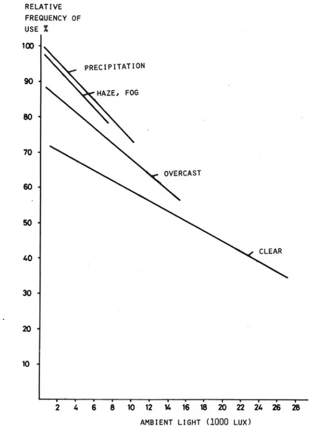
sity of the ambient light was measured every 15th minute. The relative frequency of use of running lights as a function of the ambient light during different types of weather is outlined in Figure 2. The observations were made in the winter of 1975/76 and during different types of weather outside built-up areas in the counties of Usterg tland and Stidermanland (in 10 different locations).

RELATIVE FREQUENCY OF USE Z 100

AMBIENT LIGHT (1000 Lux)

Figure 2. Relative frequency of use of running lights as a function of ambient light during daylight for different types of weather

conditions in 1975/76.

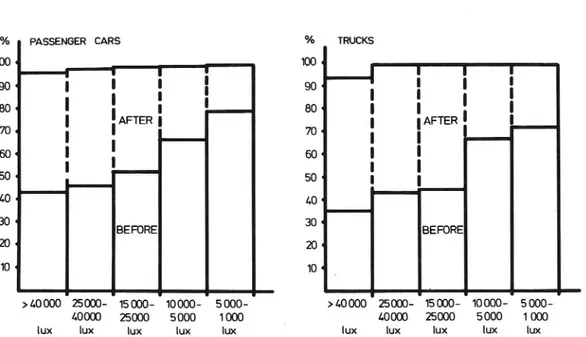
In some of these locations passenger cars and trucks were dealt with separately.

In Figure 3, the use of running lights by passenger cars and trucks is shown as it was before and after the law in relation to the intensity of the ambient light.

% PASSENGER CARS % TRUCKS

100 1 100 1 . I l ' I I I I 90 « | I : : go . ' : : :I l I 80 « I I 80 « | I I

I

'AFTER II

|

|AFTER |

__

I

'

I

I

I

lux lux lux lux lux lux lux lux lux lux

Figure 3. The use of running lights on E4 (European highway No. 4) in relation to ambient lighting in D-county before and after the law came into effect.

Unfortunately, the number of comparative measurements between years is rather limited (i.e. the same place, the same season and the same weather conditions) and it is therefore difficult to find a clear explanation for the variations in the use of running lights during daylight. However, the following can be verified:

The use increases with increased cloudiness The use is greatest during precipitation The use is greater outside built-up areas

The use is greater in the afternoon than before noon

The use increases when the length of daylight period decrease

As soon as the law was in effect, October 1st, 1977, the use was close to "total"

An increase in the use before the law, i.e. the summer of 1977, was not noticed. It was first during the days close to the law that a noticeable increase occurred

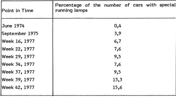
In connection with the Swedish Road Safety Office's measurements, the use of special running lamps was also recorded.

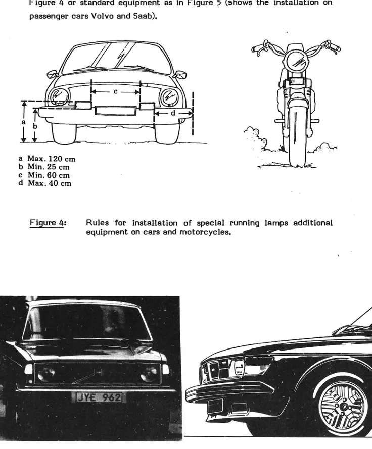
These special running lamps are of two kinds, additional equipment as in Figure 4 or standard equipment as in Figure 5 (shows the installation on passenger cars Volvo and Saab).

Figure 4: Rules for installation of special running lamps additional equipment on cars and motorcycles.

Figure 5: Passenger cars of Volvo and Saab standard equipped with special running lamps.

Percentage of the number of cars with special Point in Time running lamps

June 1974 0,4 September 1975 3,9 Week 16, 1977 . 6,7 Week 22,1977 7,6 Week 29, 1977 9,5 Week 34, 1977 7,6 Week 37, 1977 9,5 Week 39, 1977 13,3 Week 42, 1977 15,6

Volvo's and Saab's passenger cars, which are "standard equipped" are o_t included in the above tableau. During the first year of the law, these standard equipped passenger cars accounted for approximately 10 % of the registered passenger cars, which means that close to 30 % of all passenger cars had some kind of special running lamps during the first year of the law.

As mentioned earlier, it is very difficult to make a comparison between the use of running lights before and after the law came into effect. A simple analysis of the Swedish Road Safety Office's measurements is shown in Table 1. The results include all observations within the same two-hour period made in the same places and during the same type of weather. The range of variation between different places and two hour periods is shown within brackets.

Table 1 refers predominantly to summer conditions. The range of variation reflects both the observed environment and the increase in use which occurred during the days before the law came into effect. The tables, however, reflect the conditions during the summer periods before the law, whereas the after-the-law results mainly come from measure-ments during the winter periods.

10

However, Table 1 clearly underlines the effect of the law itself, and also

reflects the influence that information and weather conditions had before the law came into effect.

In Table 2 and Table 3, an attempt has been made to divide the National Road Safety Office's observation locations into "outside built-up areas" and "inside built-up areas". As is indicated by the tables, the difference between the two settings during various weather conditions is small.

Table 1. Percentage passenger cars with vehicle lights in use during daylight and different weather conditions before and after the law during different weather conditions.

No Precipitation Intermittent Rain Rain

Before After Before After Before After

Clear 33 93 - - _ (13-85) (68 100) Partially 39 94 48 89 -Cloudy (22-74) (88-98) (23-83) (85-95) Overcast 48 97 51 96 64 94 (25-88) (83-100) (34-91) (91 100) (35-96) (87-100) Haze/Fog 53 96 76 96 74 97 (35-71) (86-100) (60-89) (95 98) (48 96) (97)

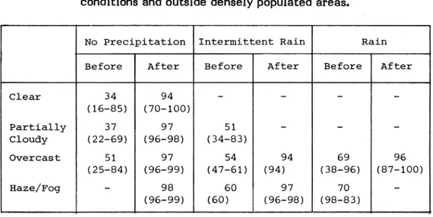
Table 2. Percentage passenger cars with vehicle lights in use during daylight before and after the law during different weather conditions and outside densely populated areas.

No Precipitation Intermittent Rain Rain

Before After Before After Before After

Clear 34 94 - -(16-85) (70 100) Partially 37 97 51 Cloudy (22-69) (96-98) (34 83) Overcast 51 97 54 94 69 96 (25-84) (96-99) (47 61) (94) (38 96) (87 100) Haze/Fog 98 6O 97 7O (96 99) (60) (96-98) (98-83) v.1 REPORT 208A

ll

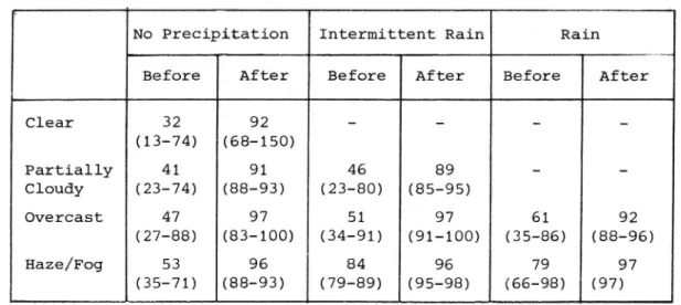
Table 3. Percentage passenger cars with vehicle lights in use during daylight, before and after the law, during different weather conditions within densely populated areas.

No Precipitation Intermittent Rain Rain

Before After Before After Before After

Clear 32 92 - - -(13-74) (68-150) Partially 41 91 46 89 -Cloudy (23-74) (88 93) (23-80) (85-95) Overcast 47 97 51 97 61 92 (27-88) (83-100) (34-91) (91 100) (35 86) (88-96) Haze/Fog 53 96 84 96 79 97 (35 71) (88 93) (79 89) (95-98) (66-98) (97)

12

DATA ON ACCIDENTS

The data on accidents are based on police-reported personal injury acci-dents during the period from October 1975 to September 1979. This means that the periods before and after the law are both two years.

The data on accidents have been divided into accidents outside built-up areas and accidents inside built-up areas and according to month and day. The accidents were classified according to the region in which they occurred: southern, central or northern Sweden.

The accident type categories are as follows: Group 1 - single motor vehicle accidents

- multiple vehicle accidents,

(i.e. head-on collisions)

- multiple vehicle accidents, crossing directions - multiple vehicle accidents, coinciding directions

- motor vehicle/pedestrian - motor vehicle/bicycle, moped

opposing directions

Group 2 - other single vehicle accidents - other multiple vehicle accidents

- motor vehicle/animal

Only accidents from Group 1 are analysed. The accidents have also been divided according to whether they occurred in daylight or in darkness. Accidents in twilight or when the light conditions are unknown, are not included in the analysis which is based on monthly results.

When the analysis was based on a 24-hour period, accidents in twilight and unknown light conditions were included in darkness accidents. In this case the accidents were recorded according to whether the period was sunny, normal or cloudy. The following geographical places were chosen from the

Swedish Meteorological and Hydrological Institute's (SMHI) monthly

re-ports: Sundsvall, Karlstad, Bromma, Norrktiping, Jiinkiiping, Landvetter,

Sval v.

13

If the number of sunny hours during a 24-hour period for the above seven places averaged out to be more than 57 % of the daylight hours, the period was classified as "sunny". If the average was less than 29 %, it was classified as "cloudy". The intervening periods were termed "normal". The reason for this classification is to be able to examine the effect of running lights during different existing ambient light conditions. Further-more, this classification increases the possibilities of a comparison between different years, asthe use of running lights before the law was influenced by the existing light conditions.

Table 4 shows the number of accidents during the four investigated one-year periods.

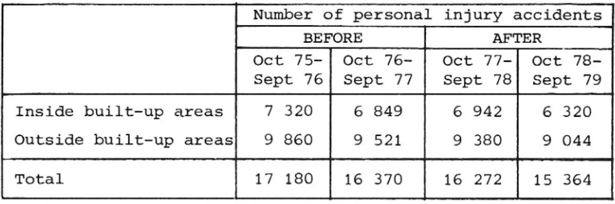
Tablet; Number of police-reported personal injury accidents inside built-up areas and outside built-up areas during the different time periods before and after the law.

Number of personal injury accidents

BEFORE AFTER

Oct 75- Oct 76- Oct 77- Oct

78-Sept 76 Sept 77 Sept 78 Sept 79 Inside built-up areas 7 320 6 849 6 942 6 320 Outside built-up areas 9 860 9 521 9 380 9 044

Total 17 180 16 370 16 272 15 364

The reason behind the compulsory use of vehicle lights in daylight was that vehicles will be noticed earlier when their lights are on.

This implies that of all accidents, the multiple accidents during daylight are the ones which will be influenced by the law.

All in all, this type of accident- constitutes more than 50 % of all police-reported personal injury accidents. Table 5 shows the percentage distribution of accidents according to inside built-up areas versus outside built-up areas, single versus multiple accidents, and daylight versus darkness during the four-year period (October l975-September 1979). VTI REPORT 208A

14

The circled numbers indicate those groups which can be affected by the use of the law. As shown in the table, 2/3 of these accidents occur inside

built-up areas and 1/3 outside built-up areas.

TableS The percentage distribution of the police-reported personal injury accidents in relation to environment, light conditions

and single (5) versus multiple (M) accidents during the period

of October 1975 September 1979.

. Light Oct. 75 - Sept. 79

Env1ronment conditions S M Inside Daylight 3,7 <::::D built-up area Darkness 4,0 14,6 Outside Daylight 9 , 4 built-up area Darkness 7,2 5,8 Total 100%

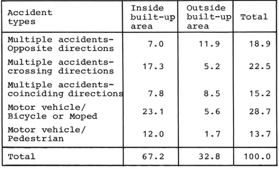
If the effect of the use of vehicle lights during daylight is different for different types of multiple accidents, the rates of different types of multiple accidents will vary between inside built-up areas and outside build-up areas. Therefore, the rate of multiple accidents inside built-up areas versus outside built-up areas might be affected differently by the use of vehicle lights during daylights. In Table 6, the percentage distribution is shown for the five different types of multiple accidents, i.e. multiple accidents - opposite directions, multiple accidents- crossing directions, multiple accidents coinciding direction, motor vehicles -bicycles or mopeds, motor vehicles pedestrians.

15

Table 6 Multiple accidents during daylight according to type of

acci-dent and environment. Percentage distribution (1975/79).

Accident Inside Outside

built up built up Total

types _{area area}

Multiple accidents-Opposite directions 7'0 11'9 18'9

UltiPle a801degts

17.3

5.2

22.5

M°t°r V8hiCle/

12.0

1.7

13.7

More than 1/2 of the multiple accidents inside built-up areas occur between motor vehicles and the combined group of pedestrians, bicyclists and mopedists.

CHANGES IN THE RATE OF ACCIDENTS DURING STUDIED

16

THE YEARS

The data in this section are compiled from official accident statistics. They show the changes in the rate of single and multiple accidents with personal injuries during daylight and darkness on a monthly basis.

SINGLE VEHICLE ACCIDENTS

Period Oct NOV Dec Jan Feb Mar Apr May Jon JUl Aug sept Total

1975/76 348 394 442 297 261 322 283 345 370 375 332 279 4048 1976/77 320 443 266 151 130 198 323 279 366 373 349 248 3446 1977/78 300 430 326 362 199 245 261 280 337 349 323 296 3708 1978/79 382 422 282 115 102 230 257 294 366 319 310 233 3307

MULTIPLE VEHICLE ACCIDENTS

Period Oct NOV Dec Jan Feb Mar Apr May JUn Jul Aug Sep Total

1975/76 1019 972 1001 868 674 717 702 981 1031 948 1170 1002 11085 1976/77 981 1058 995 739 789 732 657 890 1045 911 1051 1008 10856 1977/78 889 1059 883 797 676 638 615 899 995 943 1049 946 10389 1978/79 852 937 783 719 742 543 608 908 970 874 1028 888 9809

Since the analysis is simultaneously based on the number of single and multiple accidents during daylight and darkness, these figures are also

shown a

17

SINGLE VEHICLE ACCIDENTS, DAYLIGHT

Period Oct NoV Dec Jan Feb Mar APr May Jun Jul Aug sep Total 1975/76 150 138 164 125 109 180 158 248 295 290 210 146 2213 1976/77 138 176 90 61 63 110 198 200 292 291 214 143 1976 1977/78 131 198 131 160 119 134 158 210 276 276 217 155 2165 1978/79 198 180 119 57 60 100 151 203 300 238 204 137 1947

SINGLE VEHICLE ACCIDENTS, DARKNESS

Period Oct NOV Dec Jan Feb Mar Apr May JUn JUl Aug seg Total 1975/76 198 256 278 172 152 142 125 97 75 85 122 133 1825 1976/77 182 267 176 90 67 88 125 79 74 82 135 105 1470 1977/78 131 198 198 202 80 111 103 70 61 73 106 141 1543 1978/79 184 242 163 58 42 130 106 91 66 76 106 96 1360

MULTIPLE VEHICLE ACCIDENTS, DAYLIGHT

Period Oct NOV Dec Jan Feb Mar Apr May JUn Jul Aug sept Total

1975/76 633 423 406 484 424 574 609 898 970 .881 1001 801 8104 1976/77 593 457 420 384 528 566 558 807 985 823 924 816 7861 1977/78 551 490 358 369 489 484 530 818 924 862 918 745 7538 1978/79 539 433 364 401 535 404 507 812 908 721 889 686 7249

MULTIPLE VEHICLE ACCIDENTS, DARKNESS

Period Oct NOV Dec Jan Feb Mar Apr May; JUn Jul Aug, 539;, Total

1975/76 386 549 595 384 250 143 93 83 61 67 169 201 2981 1976/77 388 601 575 355 261 166 99 83 60 88 127 192 2995 1977/78 338 569 525 428 187 154 85 81 71 81 131 201 2851 1978/79 263 504 419 318 207 139 101 96 62 103 139 202 2553 VTI REPORT 208 A

5.1

18

ACCIDENT ANALYSIS

Some general remarks

The basic assumption behind the analysis is that the use of running lights

1)

tions. Thus the number of single-car accidents as well as the number of (RL) only affects the number of multiple accidents in daylight condi-accidents in darkness are supposed to be unaffected by the change in use of RL.

Obviously, several other factors affect the number of accidents, both single and multiple and in daylight as well as darkness. Those factors, their changes and effects are essentially unknown.

However, the effect of unknown factors can be controlled to some extent. Consider the following four groups of accidents:

SD = number of single accidents in daylight (Dzday) MD = number of multiple accidents in daylight

SN = number of single accidents in darkness (Nznight) MN = number of multiple accidents in darkness

If we study the quotient

(MD/SD)/(MN/SN)

the general effects of other factors are eliminated. By general effect we

mean

changes that are equal for single and multiple accidents in daylight changes in the relation between the number of single and multiple accidents,that are equal for daylight and darkness.

Effects that only change one group of accidents are called selective. The

quotient above expresses the selective effects. One cannot draw the

conclusion that the selective effect is caused by the law (i.e. the changed 15 accidents primarily involving two or more road users

19

use of RL). There are two reasons for this. First, other factors with selective effect may have changed. Second, if a factor (e.g. speeds) is supposed to affect all groups of accidents it is by no means clear that all groups are affected equal. As is shown later, a given effect can be divided into (or considered as a mixture of) general and selective effects. Thus, we are led to study the quotient MD-SN/SD'MN and ask ourselves: Are there other factors that have changed and can be expected to have

selective effects on accidents.

If selective effects of other factors are disregarded, the change of the quotient can be taken as a measure of the effect of the RL-law.

The following tables are based on road traffic accidents in Sweden with personal injury two years before and after the introduction of the RL-law October lst 1977. Collisions with animals, accidents Without motor vehicles involved and other unclassified accidents are excluded.

Darkness includes dusk and unknown light conditions.

Table7 Number of road traffic accidents with personal injury in Sweden

BEFORE AFTER CHANGE

Single, daylight (SD)

4 189

4 112

- 2 %

Single, darkness (SN)

3 304

2 893

- 12 %

Multiple, daylight (MD)

15 965

14 867

- 7 %

Multiple, darkness (MN)

5 976

5 379

10%

The number of accidents has thus decreased in all groups. The next table shows the quotient of multiple accidents to single accidents.

Table 8 q1 = (number of multiple accidents)/(number of single

acci-dents)

BEFORE AFTER CHANGE

Daylight (D) 3.81 3.62 - 5 %

Darkness (N) 1.81 1.86 + 3 % VTI REPORT 208A

20

Finally, the quotient between daylight and darkness gives the desired selective change.

Table 9 q2 = q1(D)/q1(N) = (MD/SD)/(MN/SN)

BEFORE AFTER CHANGE q2 2.11 1.95 - 8 %

Let us again point out that one cannot draw the conclusion that this is the effect of the RL-law. The only thing done so far is to eliminate (some of the) effects that obviously not can be a result of the RL-law. Other selective effects may have contributed to the change.

If the 8 % decrease of q2 is supposed to be a result of a selective change of the number of multiple accidents in daylight the absolute value of this change would be 1240 accidents or 620 accidents per year. In the following detailed analysis the estimate of the selective change varies

between - 460 and 1100 accidents per year (- 6 to - 13 percent)

depen-ding on method.

The mathematical model for the statistical analysis (a multiplicative poisson model) is discussed in the next chapter.

Later the analysis is differentiated for the following basic factors 0 summer/winter

o urban/rural areas 0 types of accidents

0 weather conditions

There are several reasons for such a differentiation

0 The model for the analysis assumes that accidents come from a papulation that is in some sense homogenous.

o Differentiated results are more informative (for a comparison, the

Finnish RL-law applies only in urban areas wintertime).

o Stronger conclusions can be drawn if the variation of differentiated results follows an expected pattern.

0 The method can be modified in some cases 9.9. for accidents with unprotected road users.

5.2

21

The model

Accidents are supposed to be poisson distributed, i.e.

P(X=k) = p(m,k) = mke'm/k!

, k=0, 1, . . .

where m is the expected value of the number of accidents X. Usually m is written as a product of risk )Sand exposure T, m = AT, but in the absence of traffic data we have to work with induced exposures.

Consider the following two-by-two-table of accidents

SINGLE(S) MULTIPLE(M)

DAYLIGHT (D) x(S,D) X(M,D)

DARKNESS (N) ><(S,N) X(M,N)

And the corrresponding expectations (when vehicle mileage is taken as

exposure):

SINGLE

MULTIPLE

DAYLIGHT

XS D TD

)M D TD

DARKNESS

ASN TM

RMN TN

The risks )S,D,..., A MN are assumed to follow the multiplicative

structure

SINGLE

MULTIPLE

DAYLIGHT

>SD = a

A MD = >456

(1)

DARKNESS

ASN = 9m

)MN = zap

If we assume that all X:s are >0 this model lays no other restrictions on them since we have expressed four variables with four new ones. The factors [NOS/5 can be considered as general factors since they influence at least two groups each. The interaction factor 6 is called selective since it only affects one group of accidents: multiple accidents in daylight (XMD).

22

The transformation Y: 1/6 , (5' = [$5 gives

SINGLE

MULTIPLE

DAYLIGHT

3

9. ,A'

(2)

MI

a at p at

DARKNESS

which shows that the selective interaction factor can be placed anywhere

in the two-by-two table. (1) is preferred for interpretation and (2) for

symmetry. We show both to emphasize that the interaction factor is not tied to multiple accidents in daylight.

Next, consider (1) for four different years. The expected numbers of

accidents year i, i=l,...4, are given by

SINGLE

MULTIPLE

DAYLIGHT

E(XSDI) = > iTDI

E(XMDi)=AlpisiTDi

DARKNESS

E(X5Ni) -_- aiaiTNi

E(XMNi) = i i pi TNi

If we let

Ai' =7 iTDI

0 i' = iTNi/TDI

we finally arrive at the following induced exposures model for expected

numbers of accidents:

SINGLE

MULTIPLE

DAYLIGHT

c

A; 6; d

DARKNESS

Mac.

3 ; x;' p;

23

The values of (Xi' , i and li' are of little interest and will not be given. The aim of the analysis is to make inference about 6 1". 84

The maximum likelihood estimate of 6 ; is

XMDi XSNi

SDi ><MNi

41: x

and in the case of two years the relative change 62/61 is estimated by

42/41. The corresponding percentual change is (42/41-1) 100%. This is

the estimate of the change in expected number of multiple accidents in daylight due to a change in J , i.e compared to what could be expected if 8 had remained unchanged but Mp.) had changed as they did. The ML-estimate in the case of four years is a bit more complicated.

Analysis

The numbers of accidents year i, are supposed to be poisson distributed according to a multiplicative model for expectations

SINGLE

MULTIPLE

DAYLIGHT

7 i

3i Pi 6}

DARKNESS

hiai

Aiotipi

In search for selective changes of the number of multiple accidents in

daylight from before (years 1 and 2) to after (years 3 and 4) we formulate

the following hypothesis

Ho=6l=62:63264

and the alternative

Hl=8l=32£63=84

24

We use the likelihood-ratio (L-test) to test Ho against H1. H0 is rejected when q=-2 ln(L0/L1) is too great, where LU and L1 are the

likelihood functions under H0 and H1.

For reasons of symmetry we prefer to work with the transformed model

SINGLE

MULTIPLE

DAYLIGHT

R .

X.

DARKNESS

Riki

1i uipixi

The hypotheses

Ho T1 =Y2 =73 4 4

H1 3'1 =X2 3W3 =K4

are equivalent to the old ones since the 0145;, AL are unrestricted but

>0.

The ML-estimates are in the H0 case solutions to

X

_{501 MDi 5N1 MN1=)i(1+ui+fJi+o:i(5iT)}

_1:1,,,,,4

XMDi+XMNi zxiPi(1+QiX)

Lu- 4

(3)

x

_{5N1 MN1=limi(1+/5ip}

_1:1,...,4

l

E; (XSDi+XMDi+XSNi+XMNi) = Kg, Kio tf";

In the H1 case the ML-estimates are solutions to two independent systems

of the form (3) but with two years each (i = 1,2 and i = 3,4 respectively)

In order to simplyfy formulas the accidents are written with double index SINGLE MULTIPLE

DAYLIGHT Xi1 Xi2 DARKNESS Xi3 Xi4

25

A

j, e.g.mi4=)L¢L La. Let mijo be the

value of mij when the Ho-estimates of Iraq, pxi are used and let mijl Let mii be the expected value of Xi

be the corresponding Hl-estimate.

With the notions introduced above, the likelihood-ratio test is to reject Ho

when

A A

'1

2 Nij ln(mij1/mijo)

is too large. When H0 is true, r] has approximative X 2-distribution with df=l.

When H0 is rejected the conclusion is that there has been a significant change in the parameter X or equivalently its inverse 8 . The effect on accidents is estimated by

A A

R = - 0/0.

The goodness-of-fit Ktis in the usual. way given by x 2 = (xii-$ij)2/$ij.

'26

Results

ID. = ..'::E9§E

The induced exposure technique requires that accident data come from a

homogenous population. Consequently, the material is first divided into

built-up and non built-up areas for summer and winter, (table 10).

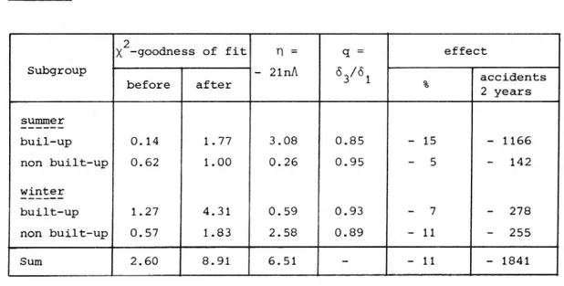
Accidents in dusk or unknown light conditions are included in darkness. Table 10. The L-test and estimated effects.

2 .

x goodness of flt n = q = effect

Subgroup - 21nA <3 /<3 . _t

before after 3 1 % :CClden 5

years EB B BEE buil up 0.14 1.77 3.08 0.85 - 15 - 1166 non built-up 0.62 1.00 0.26 0.95 5 142 BEBEEE built up 1.27 4.31 0.59 0.93 7 - 278 non built up 0.57 1.83 2.58 0.89 - 11 - 255 Sum 2.60 8.91 6.51 - - 11 - 1841

The first two columns in table 10 shows the x for goodness-of fit of the H1 model before and after. Each of them have one degree of freedom (df=1). According to the Xz-criteria, the model is accepted. It should, however, be noted that the agreement is much better for the before-period than for the after-before-period, 'X'isums are 2.60 and 8.91 respectively

(df=4).

The third column shows the values of the test variable q- JMG JLD

where L0 and L1 are the likelihood functions under H0 and H1. If H0 is true, r] has xz-distribution with df=1. None of the r, -values in table 10 is greater than the critical value 3.84 (on 5% level). The sum of the 11-values is smaller than 9.49 which is the critical value for df = 4. Thus the null hypothesis can not be- rejected or, in other words, the estimated

27

effects are not significant. The fourth column shows the quotient

A b A

Q =33/Q- ISW/Sb pnwhich expresses the selective change. Q41 means

The fact that all effects are negative makes the indication stronger that there is an effect. In fact, if H is true, the probability that all effects₀ are negative is only 2-4=0.0625. If the sign of the effect and q-values are assumed to be independent, the probability of the event that all effects

4o 0.20:0.01. This

are negative and the q-sum is greater than 6 is only

2-signs negative and the q-sum greater than a critical value) not was

formulated beforehand.

The expected effects in number of accidents during the after-period (two years) are given in the last column. The greatest contribution comes from

built-up areas, summer. The total estimated effect is a reduction of 920

accidents per year. As before, this effect is not significant. The conclusions of this section are:

0 the estimated selective change is an 11 % decrease of all multiple accidents.

0 the decrease is not statistically significant

0 the estimated change is of expected magnitude insignificancy can be

a consequence of insufficient data.

0 a combined sign- and L-test gives stronger indication that the estima-ted effects are real.

We proceed to see what information a further subdivision will bring.

28

Accident types

In the previous analyses the papulation was divided into disjoint subsets. When we turn to subdivision according to type of multiple accidents, it should be observed that all types are compared to the same set of single accidents. Therefore, the different accident-type estimations are

depen-dent.

Accidents are classifed according to primary conflict. The following types are considered:

0 opposing conflict between motor vehicles from opposing directions. 0 crossing conflict between motor vehicles from crossing directions.

0 coincident conflict between motor vehicles from coincident direc-tions.

0 cycle conflict between motor vehicle and bicycle or moped. o pedestrian - conflict between motor vehicle and bicycle or m0ped. The total sum of estimated effects in this analysis (-13 %) differs from the total sum in the previos subdivision. This is a consequense of the

non-linear model.

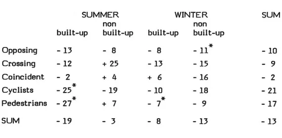
Table 11 Percentual effects by accident type.

SUMMER WINTER SUM non non

built-up built-up built-up built-up

. * Opposmg - 13 - 8 - 8 - 11 - 10 Crossing - 12 + 25 - 13 - 15 - 9 Coincident - 2 + 4 + 6 - 16 - 2

Cyclists

- 25*

- 19

- 1o

- 18

- 21

Pedestrians - 27*

+ 7

- 7*

- 9

- 17

*) Significant on the S % level.

The corresponding effects in absolute figures are given in the next table.

29

Table 12 Estimated absolute effects, number of accidents per two years.

SUMMER WINTER SUM

non non

built-up built-up built up built-up

Opposing - 84 - 66 - 37 - 117 - 304 Crossing - 199 + 90 - 153 - 51 - 313 Coincident - 14 + 30 + 27 - 93 - 50 Cyclists - 864 - 153 - 90 - 32 - 1139* Pedestrians - 363 + 11 - 6 2 - 10 - 424 SUM 1524 - 88 - 315 - 303 -2230

If running lights have any effect,greatest effect is expected for accidents

with opposing directions and smallest (no decrease or increase) for

coincident directions. The effect on accidents with crossing directions can

be expected to be somewhere in between. Accidents with cyclists and

pedestrians can also be expected to decrease with the use of running lights.

The pattern in tables 11 and 12 support this expectation: o Opposing direction accidents show a 10 % decrease.

o Crossing direction accidents decrease 9 % with some variation. 0 Coincident direction accidents decrease 2 %.

o Accidents with mopeds and cycles involved decrease 21 %. This is the greatest reduction and most of it is due to the decrease in built-up areas, summer.

0 Accidents with pedestrians decrease 17 %, also in this case a major

contribution comes from built-up areas in summer (-27 %).

Since the pattern of effects agrees with expectations the results support the hypothesis that the decrease is connected with the increased use of running lights.

30

The strong effect for accidents with unprotected road users (mopeds,

cycles and pedestrians) can be questionned. The fact that accidents with

unprotected road users decrease more than accidents involving two vehicles from opposing directions is fully acceptable on the hypothesis that peripheral vision plays an important role for unprotected road users and that running lights are important for peripheral perception.

However, the use of single car accidents as an induced measure of

exposure can be questionned. The exposure for accidents involving unprotected road users is a function of both vehicle traffic and unprotect-ed road users traffic. Since single accidents for unprotectunprotect-ed road users not are regarded, there is no induced estimate of unprotected road users

traffic.

An alternative method for analysis of accidents with unprotected road users is to make a simple two by two comparison with all accidents that are assumed to be unaffected by running lights, i.e. the sum of all accidents involving unprotected road users in darkness and single vehicle accidents in daylight and darkness.

Table 13. Accidents involving unprotected road users in daylight. Con-trol group is the same type of accidents in darkness plus single vehicle accidents.

ACCIDENTS EFFECT

GROUP c::i::g::s Control X2 accidents,

before after before after % 2 years

CYCLE E93995 built up 2788 2588 1495 1459 1.19 - 5 - 133 non built up 777 649 2991 2768 2.98 - 10 - 70 YEEEEE built-up 915 845 1793 1736 0.66 - 5 41 non built-up 150 146 2771 2578 0.14 + 5 + 6 SUM - 5 238 1 REPEETEIJ QI 539995 built-up 1014 996 1464 1450 0.02 - 1 -non built up 162 157 3012 2776 0.19 + 5 + 8 YEEEEE built-up 878 816 2313 2184 0.08 - 2 - 13 non built-up 108 100 2796 2584 0.00 0 0 SUM - 1 - 13

31

The results from this approach are given in table 13. According to the Xz-values there is no reason to reject the null hypothesis that there is no effect.

It is also possible to compare accidents involving unprotected road users in daylight with the same group in darkness. In this analysis accidents in built-up and non' built-up areas are added.

Table 14. Accidents involving unprotected road users in daylight and darkness.

ACCIDENTS EFFECT

GROUP Daylight Darkness X2

% accidents

before after before after 2 Years

SEE summer 3565 3237 355 391 6.27 - 18* - 690* winter 1065 991 899 803 0.39 + 4 + 40 s61: - 137r - 650* PEDESTRIAN summer 1176 1153 345 390 2.82 - 13 - 176 winter 986 916 1444 1257 1.18 + 7 + 58 SUM 5 - 118

The four groups in table 14 are disjoint so they can be considered as independent. In only one case, accidents involving bicycles and mopeds in summer, the change is statistically significant.

Thus, there are three possible quotients to study in order to estimate the change of accidents involving unprotected road users.

I. the quotient S in the original model (i.e. to compare the daylight to darkness ratio of studied group of accidents with the corresponding

ratio for single vehicle accidents).

11. the ratio of collisions in daylight to the sum of collisions in darkness and single vehicle accidents.

III. the ratio of collisions in daylight to darkness.

32

The estimated effects of the three methods are 1563 accidents per 2 year for the first method, - 211 for the second and 768 for the third

method.

It is satisfactory to observe that the simplest method (nr 3) gives a result

between the results of the two more sofisticated methods.

The estimated effect per year for unprotected road users thus varies between 100 and 800 accidents. Apart from this uncertainty, which is due to different methods, there is the ordinary statistical uncertainty. Only a few of the terms in the sum of accident reductions are statistically significant from zero. It follows that the statistical uncertainty is at least as great as the estimated effects.

To summarize, the estimates for different accident types and, in the case of unprotected road users, for different methods are listed in table 15. Table 15. Effects on accident types, accidents per year and percent.

SUMMER WINTER SUM

Opposing

- 75

- 77

- 152

(- 10 %)

Coinciding

+ 8

- 33

- 25

(- 2%)

Cycles

I

-508

- 61

- 569

(- 21 %)

H

-101

- 18

- 119

(- 5%)

III

-345

+ 20

- 325

(- 13 %)

n

o

- 6

-

6

(- 1 0/6)

HI

- 88

+ 29

- 59

(- 5 06)

SUM

I

-806

-309

-1115

(- 13 0/6)

II

-223

-236

- 459

(- 6 %)

III

-555

-l63

- 718

(- 9%)

Numbers that are significantly different from zero when individually tested are asterisked. It is clear that the total effect is not significantly

different from zero.

33

Weather-light conditions

A subdivision according to the weather gives the following percentual effects

Table 16 Percentual changes by weather

SUMMER WINTER SUM non non

built-up built-up built-up built-up

sunny -24 + 1 - l - 10 -15 normal - 3 - 25- 16 + 3 -ll cloudy - 9 + 25 5 - 14 - 5 Sum - l3 - 7- 8 - 10 10 None of the figures in table 16 are significantly different from zero. The pattern in table 16 is quite random. The sum-column indicates a weaker effect for cloudy days than for sunny and normal days. This is not I surprising if the effect per vehicle is assumed to be weakest for sunny days. Because of this expectation, the use of running lights before the law was highest when the expected effect was highest i.e. on cloudy days. And in the after period, the use was near 100 % in all cases. 50 the increase in use is reciprocal to expected effect per vehicle, and thus it is not possible to say which weather condition should present the greatest reduction. However the tendency in the sum column indicates that the average driver underestimated the effect of running lights in good weather conditions.The fluctuations in table 16 demonstrate the uncer-tainty of the method when the material is small.