Analysis of octamethylcyclotetrasiloxane and decamethylcyclopentasiloxane in wastewater, sludge and river samples by headspace gas chromatography/mass spectrometry

(1)

THESIS

ANALYSIS OF OCTAMETHYLCYCLOTETRASILOXANE AND

DECAMETHYLCYCLOPENTASILOXANE IN WASTEWATER, SLUDGE AND RIVER SAMPLES BY HEADSPACE GAS CHROMATOGRAPHY/MASS SPECTROMETRY

Submitted by Yu Zhang

Department of Civil and Environmental Engineering

In partial fulfillment of the requirements For the Degree of Master of Science

Colorado State University Fort Collins, Colorado

Summer 2014

Master’s Committee:

Advisor: Pinar Ömür-Özbek Kenneth Carlson

(2)

(3)

ii ABSTRACT

ANALYSIS OF OCTAMETHYLCYCLOTETRASILOXANE AND

DECAMETHYLCYCLOPENTASILOXANE IN WASTEWATER, SLUDGE AND RIVER SAMPLES BY HEADSPACE GAS CHROMATOGRAPHY/MASS SPECTROMETRY

Siloxanes are commonly used in cosmetic and personal care products, healthcare products and many industrial applications. Because siloxanes are persistent, they end up in the wastewater and go untreated through the wastewater treatment units, which lead to contamination of the surface waters through effluent discharge. Siloxanes tend to be adsorbed onto or absorbed by the

activated sludge in the wastewater treatment process. In the digesters, the siloxanes volatilize and accumulate in the biogas, which leads to mechanical problems due to scaling. The two most common siloxanes detected in wastewaters and sludge are: octamethylcyclotetrasiloxane (D4) and decamethylcyclopentasiloxane (D5).

For this study, the D4 and D5 in wastewater and sludge samples were monitored using headspace gas chromatography/mass spectrometry. Samples were collected from the City of Loveland Wastewater Treatment Plant (WWTP), Loveland, CO and the Drake Wastewater Reclamation Facilities (WWRF), Fort Collins, CO. The levels of D4 were in the range of 0.7-11.3 ng·mL-1 in wastewater and 0.3-1.8 µg·g-1 dry solid in the sludge from Drake WWRF; 1.0-6.7 ng·mL-1 in wastewater and 0.3-1.7 µg·g-1 dry solid in the sludge from Loveland WWTP. D5 levels were determined in the range of 0.4-10.4 ng·mL-1 in wastewater and 3.2-31.4 µg·g-1 dry solid in the sludge from Drake WWRF; 0.5-14.0 ng·mL-1 in wastewater and 2.5-18.9 µg·g-1 dry solid in the sludge from Loveland WWTP. The concentrations of D4 and D5 were higher in this study compared to other researches in other countries and the concentrations in waste activated sludge

(4)

iii

were in a comparable range. The concentrations of D4 and D5 in the receiving water body near the discharging points were below the limit of detection. The average mass loadings in the influent were 53.1 and 159.9 g·d-1 of D4 and 155.3 and 225.3 g·d-1 of D5 respectively in two plants.

(5)

iv

ACKNOWLEDGEMENT

Thereare many people to thank for helping me during the research work and completion of this thesis. First, I would like to thank my advisor Dr. Pinar Ömür-Özbek for her guidance,

encouragement, support and patience to make this research come true and completed. I would like to thank Dr. Greg Dooley for helping me set up the equipment and teaching the operation system. I am also grateful for Dr. Ken Carlson, who taught me the chemistry in environmental engineering. I also would like to express my thank and gratitude to John McGee from City of Loveland Wastewater Treatment Plant, who taught me the wastewater treatment plant operation, provided the opportunity to work with you and gave big support to this research. I would like thank Brian Cranmer for helping setting up the equipment and explaining the operation of the equipment. I also express my gratitude to my colleague Harshad Vijay Kulkarni, who trained me to use the lab, explained the research process and led my passion towards to this research field. I would like to thank Keerthivasan Venkatapathi, who was also one of my colleagues and shared the same lab with me. I also thank my friends who encourage and support me during studying in the US. I would like to express the most special gratitude to my parents and my family who provide support and encouragement for me to study and work, without which none of this would have been possible.

(6)

v

TABLE OF CONTENTS

ABSTRACT ... ii

ACKNOWLEDGEMENT ... iv

LIST OF TABLES ... vii

LIST OF FIGURES ... xi

Chapter 1. Introduction ... 1

Chapter 2. Literature Review ... 3

2.1 Siloxanes ... 3

2.2 Siloxanes in the Environment ... 8

2.3 Impacts of Siloxanes of Environment ... 10

2.4 Impacts of Siloxanes on Wastewater Treatment Utilities ... 12

2.5 Treatment/Romoval of Siloxanes ... 14

2.6 Detection and Analysis of Siloxanes ... 15

Chapter 3. Problem Statement ... 19

3.1 General Statement ... 19

3.2 Goal of This Study ... 21

Chapter 4. Analysis of Octamethylcyclotetrasiloxane and Decamethylcyclopentasiloxane in Wastewater, Sludge and River Samples by Headspace Gas Chromatography/Mass spectrometry ... 22

4.1 Introduction ... 22

4.2 Materials and Methods ... 23

4.2.1 Chemicals and glassware ... 23

4.2.2 Stock Solutions and Calibrations Curves ... 24

4.2.3 Sample Collection and Preparation ... 25

4.2.4 Method Validation ... 26

4.2.5 HS-GC/MS Analysis ... 27

4.2.6 Total Solids Analysis ... 28

4.3 Results and Discussions ... 28

4.3.1 Method validation ... 28

(7)

vi

4.3.3 Results of Total Solids of Sludge... 38

4.3.4 Results of Drake Wastewater Reclamation Facility, Fort Collins, CO... 40

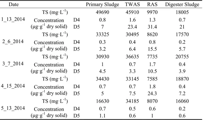
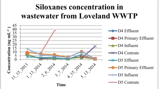
4.3.5 Results of City of Loveland Wastewater Treatment Plant, Loveland, CO ... 42

4.3.6 Concentration Comparison ... 46 4.4 Conclusions ... 48 References ... 49 Appendix ... 55 A. Raw Data – D4 ... 55 B. Raw Data – D5 ... 74 C. Raw Data – M4Q ... 93

D. Total Solids Analysis ... 110

E. Awareness Survey ... 113

(8)

vii

LIST OF TABLES

Table 2-1: Common Uses of Siloxanes and Silicones (Dewil et al., 2006) ... 4

Table 2-2: Physical Properties of Common Siloxanes (Mcbean, 2008) ... 5

Table 2-3: Structures of Siloxanes (Kaj et al, 2004) ... 6

Table 2-4: Water Solubilities of Cyclic Volatile Methylsiloxanes(Varaprath et al., 1996) ... 7

Table 2-5: Concentrations of Silxoanes in Some Species in Norwegian Lakes (Borga et al., 2013) ... 9

Table 2-6: Ion Selected for the Analysis of Siloxanes ... 18

Table 4-1: Retention Times and Ion Ratio ... 28

Table 4-2: Correlation Coefficient of Calibration Curves ... 29

Table 4-3: Average Peak Areas, Standard Deviation of Areas and Coefficients of Variation of M4Q ... 30

Table 4-4: Coefficients of Variation (%) of D4 in Wastewater and Sludge Standard ... 32

Table 4-5: Coefficients of Variation (%) of D5 in Wastewater and Sludge Standard ... 32

Table 4-6: Recovery of D4 and D5 in Wastewater and Sludge Samples (Mean ± Standard Deviation) ... 34

Table 4-7: Slopes of Linear Regression Equations between Concentrations and Peak Areas ... 35

Table 4-8: Peak Areas of Different Acetone Volume Added ... 35

Table 4-9: Mean Mass Rate of D4 and D5 in Drake WWRF ... 40

Table 4-10: Concentrations of Siloxanes in Sludge Samples in Drake WWRF ... 42

Table 4-11: Mean Mass Rate of D4 and D5 in Loveland WWTP ... 43

Table 4-12: Concentrations of Siloxanes in Sludge Samples in Loveland WWTP ... 45

Table 4-13: Concentrations in Wastewater Comparison with Other Studies ... 47

Table 4-14: Concentration in Sludge Comparision with Other Studies ... 47

Table A-1: Data of D4 during feasibility test on 4/4/13 ...……….………55

Table A-2: Data of D4 analysis on 5/7/13……….………55

Table A-3: Data of D4 analysis on 7/12/13………...………55

Table A-4: Data of D4 analysis for Fort Collins and Loveland on 7/18/13………..……56

Table A-5: Data of D4 analysis on 9/4/13……….………56

Table A-6: Data of D4 analysis on 9/10/13………...………56

Table A-7: Data of D4 during blank test on 9/11/13……….………57

Table A-8: Data of D4 analysis repeated on 9/11/13……….…………57

Table A-9: Data of D4 analysis on 9/12/13……….………..………57

Table A-10: Data of D4 in water analysis on 9/30/13………..…….………57

Table A-11: Data of D4 in sludge analysis on 9/30/13……….…….…58

Table A-12: Data of D4 analysis on 10/1/13……….……58

Table A-13: Data of D4 analysis with initial temperature of 60 on 10/4/13……….……58

Table A-14: Data of D4 analysis with initial temperature of 70 on 10/4/13……….……58

(9)

viii

Table A-16: Data of D4 analysis with initial temperature of 75 on 10/7/13………….………58

Table A-17: Data of D4 QAQC analysis with split ratio of 1: 20 on 10/8/13…………...………59

Table A-18: Data of D4 QAQC analysis with split ratio of 1: 20 on 10/9/13…………...………59

Table A-19: Data of D4 QAQC analysis with split ratio of 1: 20 on 10/10/13……….…………60

Table A-20: Data of D4 during feasible test of split ratio on 11/1/13……….……..…61

Table A-21: Data of D4 QAQC analysis with split ratio 1:10 on 11/2/13....………...….………61

Table A-22: Data of D4 QAQC analysis with split ratio 1:10 on 11/3/13………...…….………62

Table A-23: Data of D4 QAQC analysis with split ratio 1:10 on 11/4/13…………....…………63

Table A-24: Data of D4 Fort Collins and Loveland analysis with split ratio 1:10 on 11/16/13…65 Table A-25: Data of D4 Boulder analysis with split ratio 1:10 on 11/22/13……….………66

Table A-26: Data of D4 Fort Collins and Loveland analysis with split ratio 1:10 on 1/10/2014 ………...67

Table A-27: Data of D4 Fort Collins and Loveland analysis with split ratio 1:10 on 2/5/2014 ………68

Table A-31: Data of D4 Volume of Acetone Impact on 5/20/2014..………….…...…………73

Table B-1: Data of D5 during feasibility test on 4/4/13………74

Table B-2: Data of D5 analysis on 5/7/13……….………74

Table B-3: Data of D5 analysis on 7/12/13………...………74

Table B-4: Data of D5 analysis for Fort Collins and Loveland on 7/18/13………...………75

Table B-5: Data of D5 analysis on 9/4/13……….………75

Table B-7: Data of D5 during blank test on 9/11/13……….…………76

Table B-8: Data of D5 analysis repeated on 9/11/13……….………76

Table B-10: Data of D5 in water analysis on 9/30/13………...…………76

Table B-11: Data of D5 in sludge analysis on 9/30/13……….….………76

Table B-12: Data of D5 analysis on 10/1/13……….…………77

Table B-13: Data of D5 analysis with initial temperature of 60 on 10/4/13……….……77

Table B-16: Data of D5 analysis with initial temperature of 75 on 10/7/13………….………77

Table B-17: Data of D5 QAQC analysis with split ratio of 1: 20 on 10/8/13…………..….……77

Table B-18: Data of D5 QAQC analysis with split ratio of 1: 20 on 10/9/13…………..….……78

(10)

ix

Table B-20: Data of D5 during feasible test of split ratio on 11/1/13……….…….….…80

Table B-21: Data of D5 QAQC analysis with split ratio 1:10 on 11/2/13 ..………..……80

Table B-22: Data of D5 QAQC analysis with split ratio 1:10 on 11/3/13 .……….………..……81

Table B-23: Data of D5 QAQC analysis with split ratio 1:10 on 11/4/13…….……..……..……82

Table B-24: Data of D5 Fort Collins and Loveland analysis with split ratio 1:10 on 11/16/2013 ………..………..……83

Table B-25: Data of D5 Boulder analysis with split ratio 1:10 on 11/22/2013 …...……….……85

Table B-31: Data of D5 Volume of Acetone Impact on 5/20/2014 ……… ….……91

Table C-1: Data of M4Q analysis on 9/4/13………..……93

Table C-2: Data of M4Q analysis on 9/10/13………..…..……93

Table C-3: Data of M4Q during blank test on 9/11/13……….…….………93

Table C-4: Data of M4Q analysis repeated on 9/11/13………...….….……93

Table C-5: Data of M4Q analysis on 9/12/13………94

Table C-6: Data of M4Q in water analysis on 9/30/13………...………...……94

Table C-7: Data of M4Q in sludge analysis on 9/30/13………..……..……94

Table C-8: Data of M4Q analysis on 10/1/13………94

Table C-9: Data of M4Q analysis with initial temperature of 60 on 10/4/13...………..……94

Table C-10: Data of M4Q analysis with initial temperature of 70 on 10/4/13……….…94

Table C-11: Data of M4Q analysis with initial temperature of 80 on 10/7/13.………95

Table C-12: Data of M4Q analysis with initial temperature of 75 on 10/7/13….………95

Table C-13: Data of M4Q QAQC analysis with split ratio of 1: 20 on 10/8/13………95

Table C-14: Data of M4Q QAQC analysis with split ratio of 1: 20 on 10/9/13………96

Table C-15: Data of M4Q QAQC analysis with split ratio of 1: 20 on 10/10/13…..………96

Table C-16: Data of M4Q during feasible test of split ratio on 11/1/13………97

Table C-17: Data of M4Q QAQC analysis with split ratio 1:10 on 11/2/13……….………97

Table C-18: Data of M4Q QAQC analysis with split ratio 1:10 on 11/3/13…….………99

Table C-19: Data of M4Q QAQC analysis with split ratio 1:10 on 11/4/13……...………100

Table C-20: Data of M4Q Fort Collins and Loveland analysis with split ratio 1:10 on 11/16/13 ………..101

(11)

x

Table C-22: Data of M4Q Fort Collins and Loveland analysis with split ratio 1:10 on 1/10/14 ………..………105 Table C-23: Data of M4Q Fort Collins and Loveland analysis with split ratio 1:10 on 2/5/14 ………..………104 Table C-24: Data of M4Q Fort Collins and Loveland analysis with split ratio 1:10 on 3/5/14 ………..………106 Table C-25: Data of M4Q Fort Collins and Loveland analysis with split ratio 1:10 on 4/16/14 ………..………107 Table C-26: Data of M4Q Fort Collins and Loveland analysis with split ratio 1:10 on 5/20/14 ………..………108 Table C-27: Data of M4Q Volume of Acetone Impact on 5/20/2014………….………109 Table D-1: Data of TS for Fort Collins and Loveland analysis on 1/16/2014….………110 Table D-2: Data of TS for Fort Collins and Loveland analysis on 2/5/2014………...…………110 Table D-3: Data of TS for Fort Collins and Loveland analysis on 3/6/2014……...………111 Table D-4: Data of TS for Fort Collins and Loveland analysis on 4/16/2014……….…………111 Table D-5: Data of TS for Fort Collins and Loveland analysis on 5/20/2014……….…………111 Table E-1: Awareness Survey Results……….……114

(12)

xi

LIST OF FIGURES

Figure 2-1: Boiler Clogging by Silica Scaling (Dewil et al., 2006) ... 13

Figure 3-1: Effect of Silica Scaling on Fire Tube (Kulkarni, H. V., 2012) ... 20

Figure 3-2: Effect of Silica Scaling on Fire Tube in Drake WWRF (Photograph by Link Mueller) ... 21

Figure 4-1: Peaks and Retention Time... 29

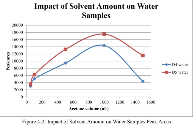
Figure 4-2: Impact of Solvent Amount on Water Samples Peak Areas………36

Figure 4-3: Impact of Solvent Amount on Sludge Samples Peak Areas………...36

Figure 4-4: Impact of Solvent Amount on M4Q Peak Areas………37

Figure 4-5: Average TS of Sludge in Loveland WWTP………39

Figure 4-6: Average TS of Sludge in Drake WWRF……….39

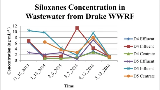
Figure 4-7: Concentrations of D4 and D5 in Wastewater samples in Drake WWRF…………...41

Figure 4-8: Concentrations of D4 and D5 in Sludge samples in Drake WWRF………...41

Figure 4-9: Concentrations of D4 and D5 in Wastewater Samples in Loveland WWTP………..44

Figure 4-10: Concentrations of D4 and D5 in Sludge Samples in Loveland WWTP………...…44

Figure E-1: Awareness Survey Questionnaire and Logics………..……113

Figure E-2: Results of Generating Biogas. ……….………115

Figure F-1: Headspace Vials with Samples (Left 2: Sludge, Right 4: Wastewater).…...………116

Figure F-2: Sludge Samples for TS Analysis (From Left to Right: RAS, Digester Sludge, TWAS, Primary Sludge) ………..……117

Figure F-3: RDT Sludge from City of Loveland……….…………118

Figure F-4: Discharge Point of Drake WWRF………119

(13)

1

Chapter 1. Introduction

The siloxanes are widely used in the daily life. They are frequently added to consumer products like cosmetics, personal care products and healthcare products. They are also present in

industrial applications (Dewil et al., 2006). Siloxanes in such products end up in the wastewater flowing into wastewater treatment plants (WWTPs). They have high volatility and low water solubility so they tend to accumulate in activated sludge. With temperature increase during anaerobic digestion, they volatilize and accrue in the biogas (Appels et al., 2008). They affect the performance of mechanical units by silica scaling, which will further increase the cost of biogas and energy generation.

With the increasing populations and the high demand for energy, the utilization of biogas is becoming one of the alternatives to the conventional fossil fuels. As a renewable energy, biogas can be beneficially used for the generation of electricity and heat. Biogas is formed by the anaerobic digestion of activated sludge in WWTPs and landfills. The anaerobic digestion also reduces the volume of activated sludge. The use of biogas for onsite generation of electricity can meet the WWTP’s own demand, which significantly reduces the cost of operation. Besides, the use of biogas also decreases the potential of the global warming by preventing emission of biogas to atmosphere (Mcbean, 2008a). In the US, there were 1351 WWTPs which have flow rates lager than 1 MGD operating anaerobic digestion in 2011. However, only 8% of these plants generate biogas for beneficial use (US EPA, 2011). The presence of impurities in biogas reduces energy generation efficiency and causes some maintenance issues. One of the impurities are siloxanes, which represent a group of silicon containing organic compounds. During combustion of biogas, siloxanes convert to silica scaling and accumulate on the inner surfaces of equipment,

(14)

2

which leads to combustion engine abrasion and damage and service interruptions. The presence of siloxanes increases the cost of operation and maintenance during the generation of energy by biogas.

Due to the occurrence of siloxanes in biogas, several removal methods have been developed, like adsorption and absorption (Schweighkofler et al, 2001). van Egmond et al. (2013) measured siloxanes in wastewater and sludge samples in a WWTP in UK. 11 WWTPs in Canada also reported the occurrence of siloxanes in influent, effluent and sludge samples (Wang et al., 2013). Removing siloxanes in the sludge and before they enter into the gaseous phase has not been fully studied. For the purpose of better evaluating the removal procedure, the analysis method of siloxanes in wastewater and sludge samples is being improved. A method for measuring siloxanes in surface water, wastewater and sludge samples was adopted and modified in this study. The concentrations of siloxanes from two utilities in Northern Colorado were also determined.

(15)

3

Chapter 2. Literature Review

2.1 Siloxanes

The name of siloxane comes from the nomenclature: Sil(icon) + ox(ygen) + (meth)ane (Dewil et al., 2006). Siloxanes represent a large group of silicones containing Si-O bonds with organic radicals bound to Si and including methyl, ethyl and other functional organic groups (UK Environment Agency, 2012). The structure of a siloxane can be linear and cyclic.

Today, siloxanes are widely used in various industrial processes, intermediate compounds for the production of other chemicals (silicone polymers), personal care products like fragrances,

lotions, shampoos, deodorants, antiperspirants, skin cleansers, nail polishes, and consumer products such as detergents, paper coatings, and textiles (Wang et al, 2012; Dewil et al, 2006). . The annual worldwide production of siloxanes is estimated at over one million tons (Hagmann et al., 1999).About 54 tons of D4 and 1670 tons of D5 are discharged to wastewater, annually in Europe (Brooke et al., 2009). Table 2-1 indicates different uses of siloxanes (Dewil et al., 2006). Siloxanes are commonly used because they are highly compressible, low flammable, have low surface tension, water repellent, high thermal stability. High temperature has limited effect on theirproperties. They have low toxicity and are not allergenic, which make them a favorable additive to the personal care products. Moreover, they are compliant with volatile organic compounds (VOC) restrictions. They are not environmentally persistent because they can be degraded in the atmosphere. They react with OH. radicals most dominantly and NO3 (nitrate ion)

radicals and ozone (Wang et al., 2012). The calculated atmospheric half-lives of D4 and D5 were reported as ~10 d and ~20 d respectively, with the assumption that fist-order kinetics was

(16)

4

over 24 h period (Atkinson, 1991). Table 2-2 illustrates the physical properties of the common siloxanes (Mcbean, 2008). The properties of methane are used as a comparison.

Hexamethylcyclotrisiloxane (D3), Octamethylcyclotetrasiloxane (D4),

Decamethylcyclopentasiloxane (D5) and Dodecamethylcyclohexasiloxane (D6) are cyclic

volatile methylsiloxanes (cVMS), while Hexamethyldisiloxane (L2), Octamethyltrisiloxane (L3), Decamethyltetrasiloxane (L4) and Dodecamethylpentasiloxane (L5) are common linear

siloxanes. cVMS have high vapor pressures, low water solubilities and high Henry’s Law constants. Due to these properties, D4 is used as an off-site intermediate for the production of silicone polymers, at the same time D5 and D6 are mainly added to personal care products. Table 2-3 shows the structures of siloxanes (Kaj et al., 2004).

Table 2-1: Common Uses of Siloxanes and Silicones (Dewil et al., 2006)

Usage Example

Medical usage

Implants in cosmetic surgery, tracheostomy tubes Coating hypodermic needles and bottle stops Coating pacemakers

Elastomer usage Silicone components and tubing Gels Barrier creams

Nappies

Adhesives

Fire retardants

Extensive usage as carrier oils Waterproofing agents Fabric softeners Paints Penetrating oils Paper products Anti-foams Personal toiletries

(17)

5

Table 2-2: Physical Properties of Common Siloxanes (Mcbean, 2008) Compound Abbreviatio_n Molecular Weight (g∙mol-1₎ Boiling Point ( ) Melting Point ( ) Vapor Pressure (kPa @25 ) Hexamethylcyclotrisiloxane D3 224.46 134 65 1.14 C12H18O3Si3 Octamethylcyclotetrasiloxane D4 296.61 175 17.4 0.13 C8H24O4Si4 Decamethylcyclopentasiloxan e D5 370.77 210 -44 0.05 C10H3O5Si5 Dodecamethylcyclohexasilox ane D6 445 245 -3 0.003 C10H36O6Si6 Hexamethyldisiloxane L2 162.4 100 -67 4.12 C6H18Si2O Octamethyltrisiloxane L3 236.5 153 -82 0.52 C8H24Si3O2 Decamethyltetrasiloxane L4 310.7 194 -68 0.073 C10H30Si4O3 Dodecamethylpentasiloxane L5 384.8 230 -81 0.009 C12H36Si5O4 Methane CH4 - 16.04 -162 -182 -

(18)

6

Table 2-3: Structures of Siloxanes (Kaj et al, 2004)

Abbreviation CAS # Structure

D3 541-05-9 D4 556-67-2 D5 541-02-6 D6 540-97-6 L2 107-46-0 L3 107-51-7 L4 141-64-8 L5 141-63-9

Table 2-4 shows the water solubilities of cyclic volatile methylsiloxanes in distilled water (Varaprath et al., 1996).

(19)

7

Table 2-4: Water Solubilities of Cyclic Volatile Methylsiloxanes(Varaprath et al., 1996) Compound Solubility _(μg∙L-1₎

D4 56

D5 17

D6 5

The organic carbon partitioning coefficient (KOC) is a physical parameter for describing transfer

of chemicals between the water and sediment or water and soil exchange. KOC is the ratio

between the mass of a chemical which is adsorbed in the soil or sediment per unit mass of organic carbon in the soil and the chemical concentration in solution at equilibrium. Miller, (2007) reported that the value of logKOC of D4 in soil was 4.22. The values of logKOC of D5 was

indicated by van Egmond and Sanders (2010) to be 5.6-5.7 for the natural soil, 5.2-5.4 for the natural sediment and 5.4-5.5 for the artificial sediment.

The octanol/water partition coefficient (KOW) is defined as the ratio between the concentration of

chemical in a unit volume of n-octanol (a non-polar solvent) and the concentration in a unit volume of water ( a polar solvent) after the octanol and water have reached equilibrium (Smith et al., 1988). The values of logKow of D4 and D5 were measured by Bruggeman et al. (1984) as

4.45 and 5.20, respectively, by a high performance liquid chromatography retention time method. Using a slow-stirring method for multi-phase quilibrium in a closed system, the values of logKow of D4 and D5 were determined as 6.49 and 8.03 by Kozerski) (2007) and7.0 and 8.07

for D4 and D5, respectively by a dual-syringe system method for multi-phase equilibrium in a closed system by Kozerski and Shawl (2007). Because both logKOC and logKOW forD4 and D5

are greater than 4, they have a strong tendency to bind to soil and sediment with high organic matter.

(20)

8 2.2 Siloxanes in the Environment

Siloxanes mostly volatilize into the atmosphere from personal care product and health care products, where they are decomposed into silanols and various carbonyl compounds (Muller et al., 1995). Some of them end up in the wastewater and hence at the wastewater treatment plants (WWTPs), where they cannot be degraded by the activated sludge treatment employed by the WWTPs. Siloxanes are not very soluble in water but they tend to adsorb onto organics. After the activated sludge process, siloxanes stay in the wasted sludge that may be sent to sludge digesters for biogas production or further treatment of the sludge before disposal (Hayes et al., 2003). Due to higher temperatures in the anaerobic sludge digester, most of siloxanes volatilize and end up in the biogas (Mcbean, 2008b).

Siloxanes are hard to remove from wastewater completely, so they could be discharged into the surface water bodies. It was reported by Mueller et al. (1995) that 0.06-0.41 µg·L-1 of D4 was detected in effluent of WWTPs in US. About <0.06-3.7 µg·L-1 of D4 and <0.04-3.8 µg·L-1 of D5 in wastewater were determined in Nordic environment (Kaj et al., 2005b). <0.01-0.029 µg·L-1 of D5 were detected in two rivers in Eastern England (Sparham et al., 2008). <0.009-0.023 µg·L-1 of D4 and <0.027-1.48 µg·L-1 of D5 in a river in Canada (Wang et al., 2012). In the aquatic environment, siloxanes tend to be degraded very slowly and bioaccumulate in fish (Brooke et al., 2009). D5 was detected in fish in several surface waters which receive effluents from WWTPs in Nordic countries, such as the Oslo Fjord (Kaj et al, 2005a), the Rhine River (Brooke et al., 2009), and the Svalbard (Warner et al, 2010). Traveling with the surface waters, siloxanes were found in the flesh of the fish in other water bodies far from the effluent discharge points. For example, D4, D5 and D6 at 10, 200 and 40 ng∙g-1 lipid weight concentration, respectively, were determined in herring in many locations in the Baltic Sea which didn’t receive any effluent from

(21)

9

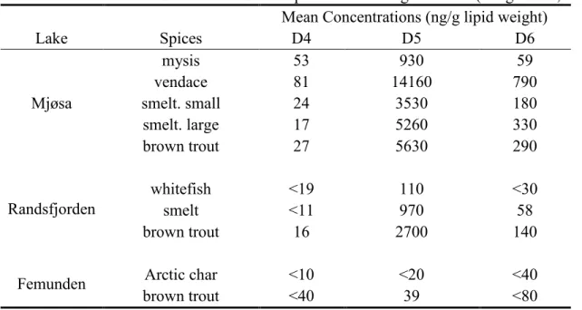
WWTP directly (Kierkegaard et al, 2012). As shown in Table 2-5, siloxanes were found in different species from lakes in Norway (Borga et al., 2013). D5 dominated the major

contaminant among siloxanes in these species due to the large usage of D5. It was also reported that 0.8-14.4 ng∙g-1 wet weight of D5 was present in perch from six Swedish lakes that received WWTP effluent (Kierkegaard et al., 2013). Bioaccumulation of siloxanes could occur to human by consumption of fish contaminated by siloxanes.

Table 2-5: Concentrations of Silxoanes in Some Species in Norwegian Lakes (Borga et al., 2013) Mean Concentrations (ng/g lipid weight)

Lake Spices D4 D5 D6 Mjøsa mysis 53 930 59 vendace 81 14160 790 smelt. small 24 3530 180 smelt. large 17 5260 330 brown trout 27 5630 290 Randsfjorden whitefish <19 110 <30 smelt <11 970 58 brown trout 16 2700 140

Femunden Arctic char <10 <20 <40

brown trout <40 39 <80

Siloxanes are also present in atmosphere due to the usage and emission of biogas. In a study of biogas, 4800-5100 μg ∙m-3 of D4 and 600-650 μg ∙m-3 of D5 were determined in landfill gas, and 6300-8200 μg ∙m-3 of D4 and 9400-15000 μg ∙m-3 of D5 were reported in wastewater gas

(Schweighkofler et al, 2001). D6 was reported with a concentration of 210 μg ∙m-3 in the landfill gas in Canada (McBean, 2008b). Rasi et al., (2010) demonstrated that the amount of cyclic siloxanes in different places varied greatly because of the different raw waste and wastewater, different treatment processes together with the different biogas generation processes. Compared with biogas, the concentrations of siloxanes in indoor and outdoor air were much lesser. The

(22)

10

common usage of cosmetic and personal care products dominated the typical source of siloxanes in indoor air (Gouin et al, 2013, Montemayor et al., 2013). Mean concentrations of D5 of 39.6 μg ∙m -3 , 26.1 μg ∙m -3 and 7.0 μg ∙m -3 were detected in indoor air from administrative offices, data centers and telecommunication offices in US (Shields et al., 1996). D4, D5 and D6 were

identified in 73, 250 and 142 out of 400 studied Swedish homes with mean concentrations of 9.0, 9.7 and 7.9 μg ∙m -3(Kaj et al, 2005b). Another study conducted by Steer et al. (2008) in Canada reported that 0.1-0.2 μg ∙m -3 D4 were determined in non-lab and analytical lab air and about 0.03 μg ∙m -3 in clean labs. D5 concentrations were determined at 14 μg ∙m -3 in analytical laboratory and 9 μg ∙m -3 in non-lab locations. It was concluded that higher siloxanes concentrations were present in the locations close to WWTP and in enclosed buildings (Steer et al, 2008). Because of the diffusion, the concentrations of siloxanes in outdoor air are lower than that in indoor air. It was reported that D4 was determined at trace amounts in the US atmosphere in the mid-1970s (Pellizzari et al, 1976). D5 was detected in trace concentration in the air samples from China. D3 and D4 were measured with highest concentrations in an industrial area compared to the air samples from urban, industrial, landfill, WWTP, suburban and a forest park. All of these areas except the forest park were detected the occurrence of siloxanes (Wang et al, 2001). Yucuis et al. (2013) measured the outdoor air concentrations of siloxanes in areas in Chicago, US. It was reported that 54, 17 and 9.7 ng∙m -3 of D4 and 210, 52, 18 ng∙m -3 of D5 were detected in urban, suburban and rural area respectively.

2.3 Impacts of Siloxanes of Environment

The remaining siloxanes in the wastewater effluents may be discharged to surface waters. In water bodies, siloxanes exhibit little toxicity to the organisms because of their low water solubilities (Wang et al., 2013). The large molecular size of siloxanes reduces uptake by

(23)

11

organism, but over time they will bioaccumulate. The equilibrium partitioning between the environment and organisms can be represented directly by the bioconcentration factor (BCF). The BCFs of 1090, 1010 and 1200 L∙kg -1 for D4, D5 and D6 respectively were determined for a goldfish exposure (Opperhuizen et al., 1987). Then the BCFs of 1875-10000 L∙kg -1(Annelin and Frye, 1989) and 12400 L∙kg -1 (Fackleret al., 1995) for D4, 4450 L∙kg -1 (Parrott et al., 2013) and 13300 L∙kg -1 (Drottar, 2005a) for D5 were detected in fathead minnows studies. Drottar, 2005b reported that the BCF of 1660 L∙kg -1 for D6 was estimated using fathead minnow. These researches reported BCF values for D4 and D5 were larger than 2000, which indicated D4 and D5 were bioaccumulative (BCF >2000)(European Commission, 2010).

As a result of siloxanes’ bioaccumulative property, they present toxicity to aquatic animals. Wang et al. (2012) studied the toxicity of D4 and demonstrated that D4 can be toxic to some aquatic creatures at very low concentrations (15 µg·L-1) while other organisms were not affected. Sousa et A-(1995) showed that rainbow trout was the most sensitive species to D4 at10 µg·L-1. Giesy et al. (2011) reported that D5 was not toxic to fish and water flea exposed at concentration up to its water solubility limit (17 μg∙L-1). Drottar et al. (2005) reported that D6 exhibited no biological adverse effects on fathead minnow under 49-day flow-through test conditions. The concentration of D6 analyzed was up to 4.6 μg∙L-1, which was close to its water solubility limit (5 μg∙L-1).

In sediments and soil, siloxanes present toxicity to organisms. A study of prolonged sediment toxicity on midges reported that the detected no-observed-effect-concentration (NOEC) for both percent survival and emergence were 44 μg∙g-1(Krueger et al, 2008a). . Sediments were spiked with D4 at concentrations from 6.5 to 355 μg∙g-1, and the midges exposed to the maximum concentration presented a statistically significant reduction in development. Another study about

(24)

12

exposing midges to 160 μg∙g-1 indicated that D5 presented a statistically significant reduction in development. The NOEC of D5 for midge development was 70 μg∙g-1(Krueger et al, 2008b). Because siloxanes are detected at considerable levels in water, they are under consideration by UK Environment Agency and Canadian Environmental Assessment Agency for drinking water regulations and defined harmful to the environment by Environment Canada and Health Canada. The European Commission classified D4 as Category 3 for reproductive toxicity. It was

determined by Dow Corning Corporation that D5 showed a potential carcinogenic effect in a 2-year chronic toxicity and carcinogenicity study (US EPA, 2009). In this 2-2-year research, 344 rats of 60 male and 60 female were exposed to vapor concentrations up to 450 mg·g-3 of D5 for 6 h per day, 5 d per week. The female rats exposed to 450 mg·g-3 of D5 presented a statistically significant increase of uterine tumors after 2-year exposure (US EPA, 2009).

There were not effects on human health by D4 in low concentrations reported. Looney et al, (1998) found there were no immunological effects on human volunteers by D4. In this study, 12 normal volunteers (8 males and 4 females) were exposed to 122 μg∙L-1 D4 for 1 h and their blood samples were obtained for before, immediately after, and 1, 6, 24 h postexposure. This study concluded that immunotoxic or inflammatory effects of respiratory exposure to D4 were not found (Looney et al., 1998).

2.4 Impacts of Siloxanes on Wastewater Treatment Utilities

At the wastewater treatment utilities siloxanes affect the performance of various mechanical units due to scaling. During the combustion of the biogas, in the boilers, the siloxanes are converted into abrasive microcrystalline silica, which has chemical and physical properties similar to those of glass. This material deposits and accumulates on the surface of the mechanical

(25)

13

units and becomes thicker. First, the hardness of this residue leads to the abrasion of gas motor surfaces. Then since siloxanes are thermal and electrical insulators, they decrease the heat

transferring efficiency of boilers and fire tubes. Due to this layer, the demand of biogas increases to meet the same energy generation. Accumulation leads to the overheating of sensitive motor parts and depresses the function of spark plugs. It leads to serious motor damage and shortening of operation time (Appels et al., 2008). . Finally, frequent-monitoring, cleaning and repair of engines is required to prevent damages to valves, pistons rings, liners, cylinder head, spark plugs and turbocharges. Many wastewater treatment plants which utilize the biogas for energy

production face these problems. In Trecatti (UK), a major engine failure was caused by the presence of less than 400 mg/m3 of volatile siloxanes during 200 hours of operation(Griffin, 2004). Figure 2-1 illustrates the deposition of silica scaling in a boiler (Dewil et al., 2006).

Figure 2-1: Boiler Clogging by Silica Scaling (Dewil et al., 2006)

In US, 43% of wastewater treatment plants greater than 1 MGD (million gallons per day) apply anaerobic digestion but only 8% of them use biogas to generate electrical or thermal energy

(26)

14

(Water Environment Research Fundation, 2012). Increasing the efficiency together with the potential to generate renewable energy from wastewater is considerably significant. As a result, siloxanes are becoming more of a concern. The removal of siloxanes in the biogas and the activated sludge is needed.

2.5 Treatment/Romoval of Siloxanes

In US, 43% of wastewater treatment plants with greater than 1 MGD (million gallons per day) capacity apply anaerobic digestion but only 8% of them use biogas to generate electrical or thermal energy (WERF, 2012). Increasing the efficiency together with the potential to generate renewable energy from wastewater is considerably significant. As a result, siloxanes are

becoming more of a concern. The removal of siloxanes in the biogas and the activated sludge is needed.

D4 and D5 occupy the major portion of the siloxanes in the biogas produced during anaerobic digestion of the sludge. L2 and L3 are not likely in the biogas because they are much easier to dissolve in the water compared to D4 and D5 (Zhang et al., 2007). There are several methods to remove siloxanes from the biogas including physical, chemical and biological methods.

Adsorption using activated carbon is able to reduce the siloxanes to reach the concentration of total silicone less than 0.1 mg∙m-3 (Rossol et al., 2003). Other absorbents like alumina and silicone are also effective in removing siloxanes. Alumina has the adsorption capacity of 1.3 wt% to D4 (Lee et al., 2001).

SelexolTM (Poly(ethylene glycol) dimethyl ether) is a potential solvent, which can remove 99% of siloxanes in biogas (Wheless and Pierce, 2004). It is reported that sulfuric acid (concentration

(27)

15

≥ 48%) and nitric acid (concentration ≥65%) have removal efficiency of more than 95% for D5 (Schweighkofler et al, 2001).

Cryocondensation uses very low temperature to condense volatile siloxanes in the biogas. From the melting point shown in Table 2, it is easy to understand that with low enough temperature, most siloxanes transform to solid phase while the methane is still in gas phase. It was reported that under -70 , the removal efficiency could reach 99.3% (Hagmann et al, 2001). However, to decrease the temperature needs a lot of energy, so it is feasible only for the biogas with a high concentration of siloxanes (Xu et al, 2012).

Biological degradation is also feasible for the removal siloxanes. But the degradation process takes months to reach low removal efficiency (Xu et al., 2012, Popat et al., 2008, Accettola et al., 2008) .

Peroxidation is a useful method for the removal of siloxanes from waste activated sludge (Appels et al., 2008). Three oxidants were analyzed and compared: hydrogen peroxide (H2O2), POMS

(H2SO5) and dimethyldioxiranes (DMDO). All of methodologies showed an approximately 50%

removal efficiency of D4 and D5, except for the DMDO peroxidation of D4, which can remove up to 85%.

2.6 Detection and Analysis of Siloxanes

Siloxanes have been measured in many matrices, like sludge, water and soil. Dewil et al. (2007) quantified D4 and D5 in sludge samples from the secondary clarifier. The siloxanes in the sludge were extracted with n-hexane. Then the siloxanes were analyzed by a Varian 3400 gas

chromatograph coupled with a FID detector. A Varian Factor Four VF-1MS capillary column was used for the separation. The injector port temperature was set at 125 . The initial oven

(28)

16

temperature was 60 which was held for 4 min. After that the temperature was linearly increased to 250 at a rate of 8 ∙min-1_{. This temperature was kept for another 15 min. The} detector temperature was set at 250 . The detected concentrations of D4 and D5 were 0.9 mg·g-1 dry solid and 0.58 mg·g-1 dry solid respectively (Dewil et al., 2007).

The GC/MS analysis was performed for the analysis of cyclic and linear siloxanes in soil by Sanchez-Brunete et al., (2010). In this study, siloxanes were extracted with n-hexane and quantified with a GC/MS equipped with a fused silica capillary column ZB-5MS. The injector port temperature was at 200 . Helium gas is the carrier gas which has a flow rate of 1.0

mL∙min-1_{. The initial oven temperature was 40 for 2 min. Then the temperature was increased} to 220 . The mass spectrometric detector was used in electron impact ionization mode with an ion source temperature of 300 and a quadrupole temperature of 150 . The

tetrakis(trimethylsilyloxy)silane (M4Q) was used as the internal standard. This study concluded that 9.2-56.9 ng·g-1 of D5 and 5.8-27.1 ng·g-1 of D6 were detected in agricultural soils and 22-184 ng·g-1 of D5 and 28-483 ng·g-1 of D6 in industrial soils. D4 were found in only one of those industrial soil sample with a concentration of 58.6 ng·g-1, but not in any of the agricultural ones (Sanchez-Brunete et al., 2010).

Another analysis method was applied to determine the concentrations in soil and sludge samples which was concurrent solvent recondensation – large volume injection – GC/MS (CSR-LVI-GC/MS) done by Companioni-Damas et al. (2012). The extraction procedure was applied as following: First, 0.5 g sample equilibration stayed at 4 overnight. Second, it was mixed with 2 g of anhydrous sodium sulphate for 3 hours. Third, it was shook for 10 min with 3 mL n-hexane containing 0.2 g of activated Cu. Finally, it was centrifuged at 3500 rpm for 10 min. J&W DB-5MS capillary column (60m×0.25 mm, 0.25 um film thickness) was used for GC analysis. The

(29)

17

GC injector was set on splitless mode and operated at 60 initial temperature holding for 5 min, then heated up to 285 at 10 /min holding for 15 min. This analysis method achieved good linearity (R>0.9993) and recoveries ranging from 80% to 100%. This study obtained 2528-15,070 ng·g-1 dw of D4, 2106-82,112 ng·g-1 dw of D5 and 1840-11,935 ng·g-1 dw of D6 in sludge samples. The concentrations of D5 and D6 in urban soil samples ranged from 11-30 ng·g

-1_{dw and 7.2-47 ng·g}-1_{dw, respectively. Concentrations of D4 in urban soil samples were under}

limit of detection (Companioni-Damas et al., 2012).

The analysis of siloxanes in water has been performed by Headspace-GC/MS method by Sparham et al., (2008). For this method, extraction was not necessary because siloxanes volatilize into the headspace and were pressurized through the inlet onto the GC coupled with MS. Ultrapure water and 20 mL headspace glass vials were used. First the sample was heated at 80 for 10 min for equilibrium. Then 3 mL of the headspace was injected via the GC injector which has a temperature at 250 . After keeping the initial temperature at 40 for 4 min, the oven was heated to 200 at 8 ∙min-1_{and held for 5 min, before heating to 250 at 20 ∙min} -1_{. Finally the MS detector was operated using single ion monitoring. The internal standard was} [13C5]decamethylcyclopentasiloxane (13C5–D5). In this study, a non-siloxane-based column was

used which is a polyethylene glycol- based stationary phase DB-Wax column, that gives a more accurate result. The detected concentration of D5 was <10-30.6 ng·L-1 in the river samples and 31-400 ng·L-1 in the treated wastewater samples (Sparham et al., 2008).

Companioni-Damas et al. (2011) conducted the analysis method to measure the concentrations of siloxanes also in water using headspace-solid phase microextraction (HS-SPME) and GC/MS. 20 mL water sample was spiked into a 40mL screw cap glass vial which was fitted with black Viton septa. The septa contained a stainless steel rod10 mm×5mm PTEF-coated stir bar. After 3 min

(30)

18

vortex mixing and 10 min 25 water bath, the samples were extracted with a 65

µm-PDMS/DVB fiber at 25 for 40min using a constant magnetic agitation rate of 750 rpm. Then the fibers were exposed in the GC injector port at 240 for 5 min in order to reach thermal desorption. DB-5 MS fused silica capillary column (60 m ×0.25 mm I.D., 0.25 µm film

thickness) was applied on GC. GC oven was held at 40 ◦C for 2 min before being heated to 250 ◦C at 10 ∙min-1_{and held for 5 min. Helium gas flow-rate was 1mL∙min}-1_{. M4Q was the internal}

standard while the acetone was solvent used for the stock solution. This method obtained good linearity (R>0.999) and low limits of quantification ranging from 0.01 to 0.74 ng·L−1 for linear siloxanes and 18-34 ng·L−1 for cyclic siloxanes. This study reported 22.9 ng·L−1 and 58.5 ng·L−1 of D5 in two testing rivers and 21.2 ng·L−1 of D6 in one of them (Companioni-Damas et al., 2011).

The mass spectrometry is the most commonly used method for detecting siloxanes because it is used to characterize, identify and quantify compounds and it provides accurate results. The mass-to-charge ratios (m/z) of D4 and D5 are shown in following Table 2-6.

Table 2-6: Ion Selected for the Analysis of Siloxanes Compound Ions Selected

(m/z) D4 133, 281 D5 267, 355 M4Q 281, 369

(31)

19

Chapter 3. Problem Statement

3.1 General Statement

Due to the high energy requirements, an increasing number of wastewater treatment plants use the biogas to generate electricity and heat. The biogas is produced by the anaerobic digestion of the waste activated sludge. The anaerobic digestion not only solves the problem of reducing the volume of waste activated sludge, but also produces biogas for beneficial usage. The

composition of biogas includes mainly methane (CH4), carbon dioxide (CO2), carbon monoxide

(CO), hydrogen sulphide (H2S), water and other impurities such as siloxanes. The occurrence of

siloxanes, which are from the cosmetics and personal care products, will convert to silica scaling (abrasive microcrystalline silica) during the combustion of biogas. The silica scaling, which has very similar chemical and physical properties as glass, tends to attach to and accumulate on the inner surface of the boilers. This material leads to attrition of the gas engine surfaces and overheating of sensitive motor parts, which may cause serious major engine failure.

The scaling process reduces the efficiency of the energy generation. Also maintenance becomes an issue because it is expensive and time consuming to clean the engine and pipeline or to replace failed equipment. The available techniques to remove siloxane in the biogas are relatively expensive, resulting the higher cost of biogas. Efficient and accurate methods to measure the amount of siloxanes in wastewater and sludge have to be developed and validated in order to achieve better evaluation of the occurrence of siloxanes and removal procedures.

City of Loveland Wastewater Treatment Plant is one of the WWTPs that has been experiencing scaling issues due to occurrence of siloxanes in biogas. The plant has 29 square miles of service area with a peak wet hourly flow rate of 11.6 MGD. The average flow rate from April to

(32)

20

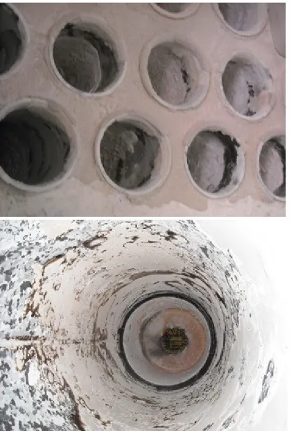
September is 6.2 MGD and during the rest of the year is 5.7 MGD. This plant operates anaerobic digestion to produce biogas for in-house heating. It was observed that the inner surfaces of the fire tubes were coated by the silica scaling after a few months. Figure 3-1 illustrates the accumulation of silica scaling on the fire tubes. The picture on left was captured in June 2010 while the right one was took in March 2011 (Kulkarni, H. V., 2012). As seen in Figure 3-2 same problem is observed by the Drake Wastewater Reclamation Facilities. These pictures were taken in 2009 during a cleaning event.

(33)

21

Figure 3-2: Effect of Silica Scaling on Fire Tube in Drake WWRF (Photograph by Link Mueller)

3.2 Goal of This Study

The goal of this study was to optimize an analysis method and to determine the occurrence of siloxanes (D4 and D5) in wastewater and sludge samples from the City of Loveland WWTP and Drake WWRF, and river samples samples over time. The adopted and modified detection method was Headspace-Gas Chromatography/Mass spectrometry (HS-GC/MS) which is one of the most commonly used methods.

(34)

22

Chapter 4. Analysis of Octamethylcyclotetrasiloxane and

Decamethylcyclopentasiloxane in Wastewater, Sludge and River Samples by

Headspace Gas Chromatography/Mass spectrometry

4.1 Introduction

Siloxanes are widely used in various industrial processes and consumer products, such as detergents, shampoos, cosmetics, paper coatings and textiles (Dewil et al., 2006). They have been produced commercially since 1940s (Hunter et al., 1946). Two most commonly used cyclic siloxanes are Octamethylcyclotetrasiloxane (D4) and Decamethylcyclopentasiloxane (D5). The annual worldwide production of siloxanes is estimated at over one million tons (Hagmann et al., 1999). They have a low toxicity to humans, which makes them a common additive to the

personal care products. After washing and showering, siloxanes from the personal care products are flushed into sewer pipelines and end up at the wastewater treatment plants (WWTPs). They are biodegradable in the atmosphere, but they are not degraded by the wastewater treatment processes. Because of their low water solubility, siloxanes accumulate in the waste activated sludge of the WWTPs and end up in the biogas if it is generated by anaerobic sludge digestion. During the combustion of the biogas, siloxanes are converted into abrasive microcrystalline silica, which has chemical and physical properties similar to those of glass, and form scales on the equipment. This residue leads to the abrasion of gas motor surfaces, overheating of sensitive motor parts and depresses the function of spark plugs leading to serious motor damage and shortening operation time (Appels et al., 2008).

Siloxanes were recognized as an issue in 1990s (Wang et al., 2013) and started to be measured in environmental samples, especially in wastewater and sludge. The average concentrations in

(35)

23

Swedish WWTPs’ sludge samples were 0.4 μg∙g-1 dry solid of D4 and 9.5 μg∙g-1 dry solid of D5 (Kaj et al., 2005). Zhang et al. (2010) reported mean D4 and D5 concentrations at 0.1 μg∙g-1 dry solid and 0.3 μg∙g-1 dry solid respectively in sludge samples from a WWTP in northeastern China. 0.1 μg∙g-1 dry solid of D4 and 15.1 μg∙g-1 dry solid of D5 were detected in the sludge in WWTP in Greece (Bletsou et al., 2013). The occurrence of siloxanes in surface waters was also reported as they are discharged with the effluents from WWTP into the receiving water bodies. In two UK rivers D5 was detected at <0.01-0.03 ug∙L-1 (Sparham et al., 2008). A study reported <0.01-0.02 ug∙L-1 of D4, <0.03-1.48 ug∙L-1 of D5 in rivers studied in Canada (Wang et al., 2012). D4 is very toxic to some aquatic organisms such as midge, daphnids and rainbow trout at very low concentrations of 6.3 ug∙L-1 (European Commission, 2010, Kent et al., 1994, Sousa et al., 1995). D4 and D5 were not a serious concern for human health but they were defined harmful to the environment due to their potential to cause ecological harm (Environment Canada and Health Canada, 2008). They are also under consideration by UK Environment Agency and Canadian Environmental Assessment Agency for drinking water regulations. D4 was classified as Category 3 for reproductive toxicity by the European Commission.

This study focused on determination of D4 and D5 in wastewater and sludge samples from two local WWTP, and river samples by Headspace-Gas Chromatography/Mass spectrometry (HS-GC/MS) analysis.

4.2 Materials and Methods

4.2.1 Chemicals and glassware

The standard solutions of Octamethylcyclotetrasiloxane (D4) and Decamethylcyclopentasiloxane (D5) were purchased from TCI-America (Portland, OR) at 98.0 % and 97.0 % purity,

(36)

24

respectively. Tetrakis(trimethylsiloxy)siloxane (M4Q) at 98% purity was purchased from Alfa Aesar (Ward Hill, MA). Acetone (99.7%) was purchased from Fisher Scientific (Pittsburgh, PA). They were all stored at room temperature in the dark except M4Q which was stored at 4 in dark.

The glass syringes at 50 μL, 250 μL, 1 mL and 10 mL were purchased from Fisher Scientific (Pittsburgh, PA). 20 mL headspace vials with flat bottoms and butyl/PTFE aluminum crimp caps (20 mm) were purchased from Agilent (Santa Clara, CA). The vials were used without any pretreatment. 1 L beakers, 500 mL flasks and 40 mL amber glass vials with screw caps were also purchased from Fisher Scientific (Pittsburgh, PA). The cap-fitted septa with diameter of 22 mm were purchased from Thomas Scientific (Rockwood, TN). Pierce hand crimper (Rockford, IL) was used to cap the Headspace vials. An Analog Vortex Mixer (No. 02215365) from Fisher Scientific (Pittsburgh, PA) was used to homogenize the samples. The disposable aluminum dishes were obtained from Fisher Scientific (Pittsburgh, PA) for the total solids determination.

4.2.2 Stock Solutions and Calibrations Curves

D4 and D5 stock solutions were prepared fresh daily in acetone for the calibration curve samples at 2 concentrations of 10 mg∙mL-1 and 42.5 μg∙mL-1. The secondary stock solutions were

prepared by successive dilution of the original stock solutions with acetone at 6 concentrations of 17 μg∙mL-1, 3.4 μg∙mL-1, 1.7 μg∙mL-1, 340 ng·mL-1, 170 ng·mL-1 and 34 ng·mL-1. M4Q stock solution was prepared in acetone at 2 μg/mL to be used as the internal standard. It was diluted to 136 ng·mL-1 to get the secondary stock solution. Then 0.5 mL of the secondary stock solution was spiked in 19.5 mL of water to achieve the final concentration of 3.4 ng·mL-1 in the final stock solution. All of these solutions were prepared in amber glass vials with Teflon line caps.

(37)

25

The calibration curve samples were prepared in sludge and distilled water samples at 0.5 ng·mL

-1_{, 1 ng·mL}-1_{, 5 ng·mL}-1_{and 15 ng·mL}-1_{of D4, 0.5 ng·mL}-1_{, 5 ng·mL}-1_{, 50 ng·mL}-1_{and 150}

ng·mL-1 of D5, 0.25 ng·mL-1 of M4Q.

4.2.3 Sample Collection and Preparation

The wastewater and activated sludge samples were collected from City of Loveland Wastewater Treatment Plant (WWTP), Loveland and Drake Wastewater Reclamation Facility (WWRF), Fort Collins CO, from November 2013 to May 2014. Loveland WWTP has an average flow rate of 6.2 MGD during April to September and 5.7 MGD during the rest of the year (City of Loveland, 2013), while the Drake WWRF has an average flow rate of 11.2 MGD during April to September and 10.2 MGD during the rest of the year. Both of the plants use activated sludge process to treat wastewater. The samples obtained were: influent, primary sludge, primary effluent, return

activated sludge, centrate, digester sludge and effluent. The water samples of Big Thompson River and Fossil Creek Ditch were collected at 1m, 10 m and 50 m from the discharging points in April, 2014. All of the samples were collected in amber glass bottles without headspace and chilled during transportation, and stored in the dark at 4 until sample preparation and analysis.

The sludge and wastewater samples were brought to room temperature for one hour. The sludge calibration curve standards were prepared as follows: 1.5 mL of waste activated sludge was placed in the headspace vial and received 1 mL of reverse osmosis (RO) water and 0.5 mL of internal standard water solution (1.5 ng·mL-1). The sludge calibration curve standards were prepared the same way, with an addition of 25 μL of corresponding D4, D5 stock to the

headspace vial to achieve concentrations of 0.5 ng·mL-1, 1 ng·mL-1, 5 ng·mL-1, 15 ng·mL-1 of D4 and 0.5 ng·mL-1, 5 ng·mL-1, 50 ng·mL-1, 150 ng·mL-1 of D5. Finally, the vials were sealed with a crimped septa cap. The sludge samples were prepared as the same manner as the sludge

(38)

26

calibration curve standards except by adding 50 μL of pure acetone instead. The wastewater calibration curve standards were prepared as follows: the headspace vials received 2.5 mL of RO water, 0.5 mL of internal standard water solution (1.5 ng·mL-1), 25 μL each of corresponding D4, D5 stock solutions with the needle just under the liquid surface to make the same headspace concentrations as the sludge standards. The wastewater samples were prepared the same way as the wastewater calibration curve standards except by adding 50 μL of pure acetone instead. Both the sludge and water blanks were also prepared in the same manner as the corresponding sludge calibration curve standards and wastewater calibration curve standards with added 50 μL of pure acetone instead to even out the volume. The concentration of M4Q in all the samples was 0.25 ng·mL-1. All the samples were tightly capped by a crimper. Then all the samples were well homogenized by the Vortex Mixer for 3 min each. Each sample was prepared in duplicates.

4.2.4 Method Validation

The following parameters, included specificity, selectivity, intermediate precision, matrix effects, linearity, limit of detection (LOD), and recovery were determined to validate this analysis

method (Huber, 2010). This procedure was performed by spiking known concentrations of D4 and D5 to blank samples (RO water and sludge), with the exception of the linearity. Triplicated samples with the same concentration was analyzed and compared to each other while the analysis was repeated for three days (Nov 2, Nov 3 and Nov 4, 2013). The concentrations series were prepared at 0, 0.1, 0.5, 1, 5, 10, 50 ng•mL-1 of both D4 and D5.Then every sample received 0.1 ng•mL-1 of M4Q. For wastewater samples, 2.5 mL of RO water and 0.5 mL of M4Q water solution were added into headspace vial. For sludge samples, 1.5 mL of waste activated sludge from Lovelan WWTP, 1.0 mL of RO water and 0.5 mL of M4Q water solution were spiked into the vial. Every sample were added 50 µL of the corresponding D4 and D5 mixture stock solution

(39)

27

except the blanks received 50 µL of pure acetone. The recovery was determined by calculating the ratio between the samples spiked known concentrations and the calculated concentration from the calibration curve equation. The spiked concentrations were 0.25, 2.5, 7.5 ng•mL-1 in both wastewater and sludge samples. Tiplicates were prepared. The HS-GC/MS analysis was conducted as the same procedure as the samples testing and described in the following section.

4.2.5 HS-GC/MS Analysis

The Gas Chromatography and Mass spectrometry analysis was performed by a Waters Quattro Micro GC/MS system. This analysis was adopted and modified from a study done by Sparham et al., (2008).The carrier gas was ultra-high purity helium at a head column pressure of 79 kPa and flow rate at 1 mL∙min-1. The GC column, J&B DB-WAX (30 m ×0.25 mm, 0.5 μm film

thickness) was purchased from Agilent. The Headspace sampler is Hewlett-Packard (HP) 7694. The headspace vials were placed in the headspace oven to heat and equilibrate for 20 min at 85 . (Other parameters: transfer line 95 , loop 105 injection time 1 min, loop equilibration time 0.01 min, loop fill 0.2 min, pressurization time 0.15 min). 2 mL of headspace was injected into the GC column with a split ratio of 1:10. The oven of GC (Agilent 6890) was held at an initial temperature of 75 , then to 100 at 5 /min, and finally to 200 at 120 /min. The MS source temperature and GC interface temperature were 220 and 280 , respectively. The mass spectrometer (Waters Quattro MicroTipleQuad) was operated in positive electron

ionization mode with selective ion monitoring for each analyte and internal standard with a dwell time of 0.1s. The electron energy and electron energy were 70 eV and 200 μA, respectively. The ions monitored were 193 and 281 m/z for D4, 267 and 355 m/z for D5 and 281 and 369 m/z for M4Q. MassLynx v. 4.1 software was used for data acquiring, integrating and processing.

(40)

28

4.2.6 Total Solids Analysis

Total solids analysis was performed for the sludge samples to report the D4 and D5 per mass of dry solids. The sludge samples (primary sludge, RAS, TWAS and digester sludge) were vortex mixed and 10 mL of each sludge sample was pipetted into a disposable aluminum dish and were dried at 105 for 24 h. Then the samples were cooled to room temperature in a desiccator, and the samples were weighed. The total solids concentration was determined by the ratio between the dried mass and the wet volume.

4.3 Results and Discussions

4.3.1 Method validation

4.3.1.1 Specificity

The sludge samples spiked with D4 and D5 were used to determine the specificity and

selectivity. To identify each siloxane analyzed, a certain retention time was observed within 1s ( 0.5-0.7%). This tolerance is smaller than that in the study done by Sanchis et al. (2013) which had a retention time tolerance of 2.5%. The ion ratios of 2 selected ions for each siloxane were checked and confirmed to stay in the same range. (D4: 281, 133 m/z; D5: 355, 267 m/z; M4Q: 281, 369 m/z). Table 4-1 shows the retention times and ion ratios for siloxanes analyzed. In the complicated sludge matrix, this method was able to identify and analyze characteristic siloxane ions selected qualitatively. Figure 4-1 shows the isolated sharp peaks and retention times for siloxanes analyzed in the sludge matrix.

Table 4-1: Retention Times and Ion Ratio Compound Retention Time (min) Ion Ratio

D4 2.38 5.00 0.42

D5 3.24 0.876 0.024

(41)

29

Figure 4-1: Peaks and Retention Time

4.3.1.2 Linearity

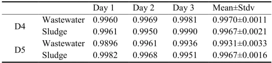
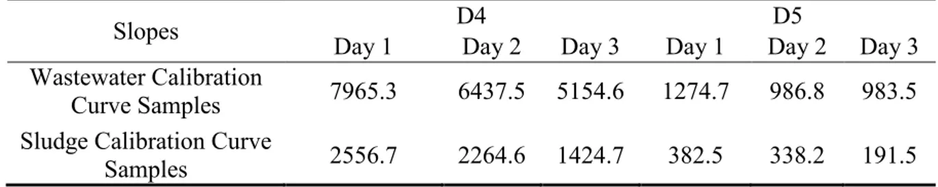
The linearity was determined by performing a 6-points calibration curve for D4 and D5 in wastewater and sludge standard samples. Calibration curve standard samples were prepared by spiking known concentrations in the wastewater and sludge samples. All the peak areas of wastewater samples were corrected by subtracting the peak areas of the blank wastewater samples while the ones of sludge samples were correceted by deleting the ones of the blank sludge samples. Then these samples were analyzed. It was observed that good linearity was showed by least squared regression (r2>0.9896). Table 4-2 shows the summary of the correlation coefficient (r2). In comparison, r2 =0.9896 of calibration curve for D5 in wastewater tested on Day 1 was slightly lower than other r2 (r2> 0.990).

Table 4-2: Correlation Coefficient of Calibration Curves Day 1 Day 2 Day 3 Mean±Stdv D4 Wastewater 0.9960 _Sludge _0.9961 0.9969 _0.9950 0.9981 _0.9990 0.9970±0.0011 _{0.9967±0.0021} D5 Wastewater 0.9896 _Sludge _0.9982 0.9961 _0.9968 0.9936 _0.9951 0.9931±0.0033 _{0.9967±0.0016} N2Acquisition Time 0.50 1.00 1.50 2.00 2.50 3.00 3.50 4.00 4.50 5.00 5.50 % -0 100

11_4_2013 siloxanes sludge 50 ngmL 2 SIR of 5 Channels EI+

TIC 2.01e6

3.38

2.38

(42)

30 4.3.1.3 Repeatability

The repeatability of this method was determined by running triplicates of water and wastewater samples spiked with M4Q at 0.1 ng·mL-1 and following the same procedure for three

consequtive days based on the guidelines of United Nations Office on Drugs and Crime, (2009) Table 4-3 shows the average peak areas and standard deviation of areas and the coefficients of variation of the internal standard. The average coefficients of variation for each day are as follows: 6.07% for Day 1, 7.85% for Day 2 and 8.43% for Day 3, which were under the requirement of validation of analytical methodology by United Nations Office on Drugs and Crime (below 20%) (United Nations Office on Drugs and Crime, 2009).

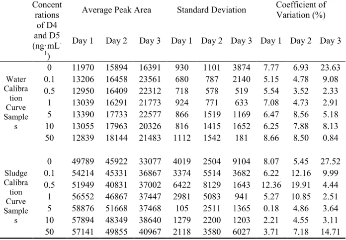
Table 4-3: Average Peak Areas, Standard Deviation of Areas and Coefficients of Variation of M4Q Concent rations of D4 and D5 (ng·mL -1₎

Average Peak Area Standard Deviation Coefficient of Variation (%) Day 1 Day 2 Day 3 Day 1 Day 2 Day 3 Day 1 Day 2 Day 3

Water Calibra tion Curve Sample s 0 11970 15894 16391 930 1101 3874 7.77 6.93 23.63 0.1 13206 16458 23561 680 787 2140 5.15 4.78 9.08 0.5 12950 16409 22312 718 578 519 5.54 3.52 2.33 1 13039 16291 21773 924 771 633 7.08 4.73 2.91 5 13390 17733 22577 866 1519 1169 6.47 8.56 5.18 10 13055 17963 20326 816 1415 1652 6.25 7.88 8.13 50 12839 18144 21483 1112 1542 181 8.66 8.50 0.84 Sludge Calibra tion Curve Sample s 0 49789 45922 33077 4019 2504 9104 8.07 5.45 27.52 0.1 54214 45331 36867 3374 5514 3682 6.22 12.16 9.99 0.5 51949 40831 37002 6422 8129 1643 12.36 19.91 4.44 1 56552 46867 37447 2981 5083 941 5.27 10.85 2.51 5 58876 51668 37468 105 2511 1365 0.18 4.86 3.64 10 57894 48349 38640 1279 2200 1203 2.21 4.55 3.11 50 57141 49855 40967 2118 3580 6027 3.71 7.18 14.71

(43)

31

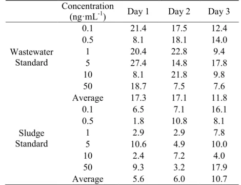
Tables 4-4 and 4-5 illustrate the coefficients of variation (CV) of target siloxanes in wastewater and sludge standard samples on three consequtive days. The CV of sludge standards was smaller than that of wastewater standards in general. The CV of sludge standards ranged from 1.1% to 17.9% while that of wastewater standards were in the range of 1.6%-37.2%. The largest CV values were observed as 27.2% of CV of D4 and 37.2 % of CV of D5 both in wastewater standard samples on Day 1. The average CV of 3-days were 15.4% for D4 in wastewater, 7.4% for D4 in sludge, 14.5% for D5 in wastewater and 9.2% for D5 in sludge. It was reported by Wang et al, (2013) that the mean CV in the analysis were 21% for D4 and D5 in wastewater samples while 8% for D4 and 6% for D5 in biosolid samples. In the study done by Bletsou et al, (2013), the CV was reported as 29% for D4 and <17% for D5 in water samples and <12% for both siloxanes in sludge samples. In this study, the mean CV in wastewater samples was much smaller and the one in sludge samples was similar compared to the discussed researches. This study exhibits good reliability for analysis. Based on these findings it was concluded that this method is repeatable, which will ensure the quality of the analysis.

(44)

32

Table 4-4: Coefficients of Variation (%) of D4 in Wastewater and Sludge Standard Concentration

(ng·mL-1) Day 1 Day 2 Day 3

Wastewater Standard 0.1 21.4 17.5 12.4 0.5 8.1 18.1 14.0 1 20.4 22.8 9.4 5 27.4 14.8 17.8 10 8.1 21.8 9.8 50 18.7 7.5 7.6 Average 17.3 17.1 11.8 Sludge Standard 0.1 6.5 7.1 16.1 0.5 1.8 10.8 8.1 1 2.9 2.9 7.8 5 10.6 4.9 10.0 10 2.4 7.2 4.0 50 9.3 3.2 17.9 Average 5.6 6.0 10.7

Table 4-5: Coefficients of Variation (%) of D5 in Wastewater and Sludge Standard Concentration (ng·mL-1) 11/2/2013 11/3/2013 11/4/2013 Wastewater Standard 0.1 20.1 3.2 13.6 0.5 1.6 9.4 11.0 1 9.7 15.2 3.3 5 37.2 13.8 15.6 10 16.1 27.2 7.7 50 33.2 16.7 5.6 Average 19.7 14.3 9.5 Sludge Standard 0.1 15.2 12.5 12.4 0.5 7.1 7.3 13.9 1 9.4 6.9 5.3 5 12.3 3.8 12.4 10 10.9 6.7 9.0 50 11.3 8.7 1.1 Average 11.0 7.7 9.0

(45)

33 4.3.1.4 Intermediate Precision

The intermediate precision represents the variations on different days (Huber, 2010). As shown in Table 4-3, it was observed that the average areas of internal standard (M4Q) in the water standards increased over the 3 testing days. There was an average of 31% rise from Day 1 to Day 2 and an average of 25% from Day 2 to Day 3 among the water calibration curve samples.

However, the M4Q areas were decreased over the 3 days in the sludge calibration curve samples: an average of 15% from Day 1 to Day 2, an average of 20% from Day 2 to Day 3. This was due to the complicated composition of sludge matrix that lowered the MS sensitivity, and that impacted the next analysis. The measurement was conducted in the same day ensuring the accurateness of the analysis.

4.3.1.5 Limit of Detection

The limit of detection (LOD) is “the lowest amount of analyte in a sample which can be detected but not necessarily quantitated as an exact value” (Huber, 2010). It is usually defined as the concentrations of analyte occupy a peak area as three times higher as that of blank noise level (Sanchis et al., 2013, Companioni-Damas et al., 2012, United Nations Office on Drugs and Crime, 2009). The wastewater blanks with pure acetone were prepared the same as the other blanks. After GC/MS analysis, the average peak areas of D4 and D5 in the blanks were selected as the noise level for LOD detection. This GC/MS analysis has LODs as follows: 0.22 ng/mL of D4 and 0.31 ng/mL of D5.

4.3.1.6 Recovery

Sludge and wastewater samples, which were from the same origin were used for the calibration curve standards, were prepared for the recovery test. Reported in Table 4-6, the recoveries of 94±4% and 98±6% were achieved for D4 and D5 in wastewater samples respectively, while