Household car ownership in urban and rural areas in
Sweden 1999
–2008
Roger Pyddoke and Christopher Creutzer – VTI CTS Working Paper 2014:21
Abstract
This paper studies household car ownership in urban and rural areas in Sweden using register data for all adult Swedes from 1999 to 2008. Data for individuals are linked to members of the same household, allowing us to estimate models of households. Multinomial ordered probit models for households’ private car ownership in Sweden are estimated and used to compare urban and rural households with respect to sensitivity of car ownership. The central result from comparing urban and rural households is that rural households are less likely to exit from car ownership and more likely to increase car ownership than
comparable urban households. This supports the notion that rural households are more dependent on their cars than urban households. Rural car ownership is also more sensitive to fuel price changes and the number of adults in the household. Compared with other countries, our results indicate that Swedish households’ car ownership is very resistant to change. The status of the previous year’s car ownership as well as car ownership status in 1999 is
dominant factors for household car ownership in 2008. Households with young adults are more likely to cease their car ownership and households with senior members are only slightly more likely to cease car ownership than middle-aged households. Households with higher income are less likely to cease car
ownership then lower income households and more likely to increase their car ownership. Permanent income, defined as the average income over the period, has a larger positive impact on car ownership than current income.
Keywords: Car ownership, household, income, fuel price, urban, rural, gender JEL Codes: D12, D31, R41
Centre for Transport Studies SE-100 44 Stockholm
Sweden
1 2014-10-14
Household car ownership in urban and rural areas in Sweden
1999
–2008
Roger Pyddoke and Christopher Creutzer
Swedish National Road and Transport Research Institute
Abstract
This paper studies household car ownership in urban and rural areas in Sweden using register data for all adult Swedes from 1999 to 2008. Data for individuals are linked to members of the same household, allowing us to estimate models of households. Multinomial ordered probit models for households’ private car ownership in Sweden are estimated and used to compare urban and rural households with respect to sensitivity of car ownership. The central result from comparing urban and rural households is that rural households are less likely to exit from car ownership and more likely to increase car ownership than comparable urban households. This supports the notion that rural households are more dependent on their cars than urban households. Rural car ownership is also more sensitive to fuel price changes and the number of adults in the household. Compared with other countries, our results indicate that Swedish households’ car ownership is very resistant to change. The status of the previous year’s car ownership as well as car ownership status in 1999 is dominant factors for
household car ownership in 2008. Households with young adults are more likely to cease their car ownership and households with senior members are only slightly more likely to cease car ownership than middle-aged households. Households with higher income are less likely to cease car ownership then lower income households and more likely to increase their car ownership. Permanent income, defined as the average income over the period, has a larger positive impact on car ownership than current income.
2
1 Introduction
In countries like Sweden where a relatively large part of the population inhabit sparsely populated areas, the car is almost indispensable for social and cultural life. This is indicated by the fact that people in these areas to a larger extent own cars than people in urban areas. The objective of this paper is to analyze determinants of household car ownership in urban and rural areas in Sweden. The emphasis is on the car as a means of transportation and not as durable goods that ultimately needs replacing. In particular, we want to know the significance of income and motoring costs for household car ownership. Yet we also examine the impact of employment-provided cars and the age of household members. Finally, determinants of car ownership in Sweden are compared with the corresponding determinants from similar studies in the UK and Ireland.
The register data we use provide us with links between married adults, adult children living with a parent and common-law spouses with common children. We cannot however identify common-law spouses without children. Furthermore we have chosen not to analyze single parent families. With this partial set of links, we are able to connect most individuals who are members of a household1. The fact that most previous literature is based on survey data, which does not cover as many individuals as register data, and that register data is becoming more available makes modeling with register data an attractive alternative.
Based on both travel survey studies and an earlier Swedish individual car ownership model (Matstoms 2002), the following facts about car ownership in Sweden are taken to be well known. Inhabitants in urban areas own cars to a lesser degree than rural counterparts
(Matstoms 2002 pp. 80-87). High-income earners are more likely to be car owners than low-income earners (Vagland and Pyddoke 2006 p. 25). Men own cars to a larger extent than women (Matstoms 2002 p. 50), but this difference has been decreasing. Today, young people in Sweden acquire cars and elderly Swedes cease car ownership to a lower extent than they did in the period 1980–1995 (Jonsson and Freijinger 2012).
Swedish car ownership and car acquisition has been thoroughly modeled by Matstoms (2002). The study used a dataset of all adult Swedes from 1980 to 1995, and the purpose was
primarily to create a robust forecasting model for probabilities of entry into and exit from car ownership from one year to another. These probabilities were modeled for a large number of subgroups of the population, for instance according to gender, municipality, and age.
Although the purpose of Matstoms’ study was not primarily to analyze determinants of changes in car ownership, a selective analysis was nevertheless presented.
Matstoms argues that age and income are decisive factors behind both entry to and exit from car ownership in this period, and that it is harder to model entry than exit. He also argues that exit seems to be a more inert process driven primarily by age and the type of area where the individual lives. Entry declines with age. In the 1980s, entry peaked in the 20-24 age bracket. Above this age, entry declined with age. The young were shown to be most likely to acquire a car, but many individuals in this age also ceased to own cars. In sparsely populated areas, this acquisition likelihood was found to be larger. Matstoms, however, found that entry declined in the youngest group during the 1990s for both men and women.
1
The links only allow us to form households when the couple is married or when common-law spouses have children together. We can also just link children above 18 years to the households.
3
Higher gasoline prices were shown to have a negative effect on entry to car ownership for several groups. The price variable was, however, eliminated when found not to be significant for many groups in a first round of analysis. Gasoline prices appear to have a stronger effect on entry in large urban areas than in rural areas. The income elasticity of entry was largest in the youngest group. For the older groups, the correlation between income and entry was significantly lower. Women’s entry was more income elastic than men’s. Matstoms also looked at geographical differences but found no distinct variables for explaining these. In contrast to the entry function, the exit function is u-shaped with respect to age. The exit propensities are largest for the youngest and oldest individuals. For the ages in between, the variation is significantly smaller. This is the same for both men and women. The form of the exit function does not change much over the 1980–1995 period.
In the international literature on the determinants of car ownership, most studies have used household expenditure data and panel data modeling to explore the determinants of car ownership. In the present study, the desire to explore rural car ownership precluded using Swedish household expenditure data as these datasets are thin in rural areas. Instead the availability of register data in Sweden was seen as a possibility. We also wanted to explore the expanded possibilities provided by panel data methods. Furthermore, a recently developed geographical criterion allowed us to use a sharper distinction between rural and urban
households than earlier studies.
Some previous studies on car ownership have adapted panel data methods. They have all emphasized the importance of past car ownership for predicting current car ownership. It has also been stressed that if state dependence (previous car ownership) is included in a model, there is a risk that unobserved heterogeneity among households may cause a bias in the estimate of state dependence. This risk is elaborated in Kitamura and Bunch (1990). The present study makes use of a modeling approach developed by Dargay and Hanly in a series of papers. They have worked with household data from the British Household Panel Survey. Dargay and Hanly (2000b) tried a new modeling approach utilizing an ordered-probit specification using 1993–1996 data to examine the issue of state dependence versus
unobserved heterogeneity. Dargay and Hanly (2000b) incorporated dependence on past experience by including lagged car ownership, whereas unobserved heterogeneity was specified as a random effects model with two alternative formulations. The results supported the importance of state dependence. In the two tested specifications of models taking account of state dependence, heterogeneity was not found to be significant.
Two different specifications of state dependence were estimated by Dargay and Hanly
(2000b): the number of cars owned in the previous year was used in the first and dummies for a lagged car ownership in the second. Including state dependence improved the fit of the model considerably, but the particular specification made less of a difference. The car dummy specification indicated some saturation – the more cars a household owns, the less likely it is to acquire additional cars.
The most important results in Dargay and Hanly (2000b) concern the influence of the following factors for households’ car ownership:
4
previous car ownership (state dependence) has a strong positive effect the number of adults in the household who are employed has a large effect whether or not the household head is a senior (over age 65) has an effect the type of area where the individual lives also has an effect
income has a large effect
Dargay and Hanly (2007) develop the analysis further and study two questions. The first is to what extent household car ownership and the individuals’ commuting behavior vary over time. To this end, they analyze changes in household structure, whether the household moved, employment status of its members, and changes of employer. The second is to what extent various factors influence the car ownership at household level.
The first question is addressed with a set of tables describing how household car ownership is adapted to changes in employment, housing, number of household members and form of commuting. The second question is answered by estimating a dynamic ordered probit model using data from 1991 to 2001.
Dargay and Hanly (2007) find that the strongest factor leading to a reduction of car ownership is that an adult member leaves the household. They also find that, on average, the number of households that increase their car ownership is larger than the number of households that reduce it. About 25 percent of the households either change employment or move. Both unemployment and retirement lead to reductions in car ownership, unemployment the most. The modeling analysis demonstrated a significant inertia of the current level of car ownership. The heterogeneity was also found to be significant, meaning that car ownership is influenced by unobserved differences between households. Furthermore, household car ownership increases with income and the number of adults, employed, and children in the household, respectively, while it decreases with purchase costs and population density and is lower for senior households and women. The number of full-time working adults has a stronger effect than the number of part-time workers, which in turn has a stronger effect than number of children.
Dargay and Hanly (2007) also find that car prices have a strong negative impact on car ownership. None of the other cost measures were found to have significant effects. In the 2007 model, the specification implies that the impact of the state variable is the same for all ownership levels, meaning that the inertia factor is the same irrespective of the previous year’s ownership level.
It is also well known that the proportion of car owners (households) who cease their
ownership each year is small (Matstoms 2002 and Dargay and Hanly 2007 p. 938). As the car is so important for mobility, rising costs of car ownership and car use as well as loss of job opportunities or income pose significant threats to household mobility. This study examines indications if this is more so for households in rural regions. In the present study, we therefore look at the impact of changes in gasoline and car purchase cost and disposable income on car ownership in Swedish data.
Nolan (2010) studies car ownership in Ireland 1995–2001, a period with high economic and social change. Her method is similar to the one used by Dargay and Hanly (2007) with data
5
from household surveys, yet she also controls for the initial condition problem. The most important factor for car ownership is found to be income and previous car ownership. Nolan analyzes two aspects of income, i.e., current and permanent income, where permanent income is the mean income in the period of the panel of each household. Permanent income is found to be more important than current income. Other determinants of car ownership are found to be age, children, education, and marital status.
In the present study, we have tried to apply as much as possible from the model of Dargay and Hanly (2007) and Nolan (2010) on a set of Swedish data. The most important difference between the models of Dargay and Hanly (2007) and Nolan (2010) and our model and data is that we construct households from register data on individuals. We therefore have much more data, as we have register data for nearly the whole adult Swedish population. We also have a new geographical criterion, enabling us to distinguish between households living in urban, rural, and sparsely populated areas. We can therefore look more closely at differences in car ownership depending on socioeconomic status and area of residence. Consequently, we can model rural car ownership. Also, compared with Matstoms, we have data for nine later years. These years cover a period with large increases in real disposable income and gasoline prices. However, without household expenditures, we have less resolution on the expenditures of the households. Finally, we add a correction for the initial value condition using Wooldridge’s (2005) method.
2 Data
The data used in this paper are selected to closely resemble the data used in Dargay and Hanly (2007) and originate from Swedish official records kept by the Swedish Tax Authorities and provided by Statistics Sweden. Thus, we have yearly observations for all individuals in Sweden over 18 years old and their children in the period 1999–2008. The data set includes – for example – information on the individuals’ age, gender, disposable income, children over and under 18 living with the individual, location of workplace, location of home and number of privately owned and employer supplied cars at the turn of the year. We also have a variable describing the individual’s employment status. However, this variable is not used since many unemployment spells are short. As mentioned above the tax records also only supply us with some of the links between individuals that are needed to identify all households.
The area of residence is classified into three types according to a criterion developed by the now terminated Glesbygdsverket (the National Rural Development Agency): individuals or households in (1) urban areas with more than 3,000 inhabitants, (2) rural areas close to an urban area with a 5–45 minute driving distance from the nearest urban area and (3) sparsely populated areas with a driving time from the nearest urban area of more than 45 minutes. The sparsely populated areas are found almost exclusively in the northern parts of Sweden.
In 2008, there were 7.354 million individuals in the dataset. Of these, 5.7 million lived in urban areas, 1.53 million in rural areas close to an urban area, and 0.11 million in sparsely populated areas. Moreover, there were 3 million car owners: 2.2 million in urban areas, 0.75 million in rural areas close to an urban area, and 0.05 million in sparsely populated areas. From these individuals, we have successfully linked together and formed 1.8 million households: 1.35 million urban households, 0.44 million rural households close to an urban area, and 0.03 million households in sparsely populated areas.
6
The links between individuals allow us to identify married couples, individuals in cohabiting couples with common children and finally parents and living with adult children. We use data only for couples who were couples for the entire period. We have therefore defined
households as consisting of a couple that is either married, or unmarried but cohabiting and having common children, and possibly adult children living with the couple. By counting all adult individuals, we may control for individuals in the household who theoretically can use a car. Among all adults, we can only distinguish those who have the above links. Therefore, our households are only a subset of all households, albeit a large subset. Our households comprise more than 6 million individuals and hence two-thirds of the population. Although we know how many minors (below 18 years of age) are associated with an adult, we cannot know whether the children stay with that parent all the time. The reason is that child custody is often shared by parents who have split up. We have therefore not used the number of minor
children in our estimates. The large set of register data allows us to merge our observations into panel data and thereby control for unobservable heterogeneity using a random effects model.
There are several potential benefits of using household data rather than individual data. Individuals are part of households and if more than one member in a household can use a car, the likelihood of that household owning one or more cars increases. We are also likely to use an irrelevant measure of income since if the members of a household may share income and durables like cars, the household income should be a more correct measure than the
individuals’ income. If households then register their cars on a single individual, it will bias the estimates of individual ownership.
Since a previous study (Matstoms, 2002) has examined the time period 1980–1995, we will in this paper study the period 1999–2008. We use a geographic characterization of areas that make it feasible to distinguish between urban, rural, and sparsely populated areas. This allows us to study the influence of population density on car ownership.
Real gasoline prices are collected from the Swedish Petroleum & Biofuel Institute and the car purchasing index price is provided by Statistics Sweden. The disposable income of an
individual is defined by Statistics Sweden and is calculated using a wide range of incomes and transfers net of tax payments.
Ideally we would also like to associate car ownership with access to public transport. There are however no such data readily available.
Diagram 1 presents income distributions for individuals above 18 years of age with a positive income, by area types and nationally. The density beyond the double median income is represented by one mass point. The most distinctive difference between the area types is that in sparsely populated areas, there are more inhabitants with lower than median disposable incomes than in the other area types. This may partly be explained by the fact that there are more elderly inhabitants in sparsely populated areas. Note the median income for individuals of 179,883 SEK.
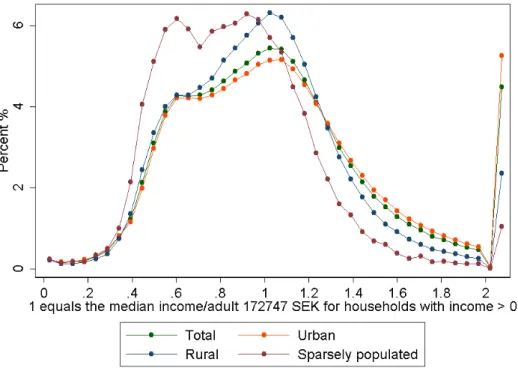
Diagram 2 also presents income distributions, but now for households. Note that the median income per adult for households is a bit lower: 172,747 SEK. Just as individuals, households in sparsely populated areas have a significantly lower income than the other two areas, with households in urban areas earning the most. The same explanation as in the individual case
7
should be applicable on our created households, with young households moving to more populated areas and less populated areas having a larger share of older people.
Diagram 1 Individual disposable income distribution in different area types
Diagram 2 The distribution of households’ disposable income per adult in different area types
Car ownership
In the total adult population, 41 percent owned cars in 2008. A strong gender pattern can be noted, with 53 percent of men and 30 percent of women owning a car. 81.1 percent of the created households own at least one car. This can be compared with the share of households that say they have access to at least one car, which was 85 percent in the travel survey data from 2012 (Trafa/RVU).
8
Car ownership is strongly correlated with disposable income and gender, as shown in Tables 1 and 2. “Total” indicates the total individual car ownership.
Table 1 Private car ownership in Sweden 2008 for disposable income quartiles, percent Total Men Women Households
Quartile 1 15.4 20.3 12.0 71.3 Quartile 2 36.5 365 1,4 50.5 26.8 84.3 Quartile 3 51.8 63.3 41.4 86.7 Quartile 4 59.7 66.1 46.7 81.9
Table 2 Private car ownership in Sweden 2008 in the three studied area types, percent Total Men Women Households
Urban Area 38.5 50.8 29.3 80.1
Rural Area 49.3 58.6 39.7 83.9
Sparsely populated area 46.4 55 37.3 79.7
Table 3 The share of private car owners in 2008 and private car owners in 2007 who ceased to own a car in 2008
Share of car owners/households
per disposable income quartile Share of car owners/households that ceased to own a car
Area 1 2 3 4 1 2 3 4 National 15.4 36.5 51.8 59.9 10.3 7.1 5.3 4.7 Urban 12.7 32.6 49.0 58.8 12.1 7.8 5.5 4.9 Rural 24.0 50 60.6 63.8 7.3 5.3 4.4 4.2 Sparse 27.6 51.8 58.2 56.3 6 5 4.3 4.3 Urban Men 17.1 47.0 62.0 66.1 12.4 6.5 4.5 4.4 Rural Men 30.9 61.3 67.7 66.3 6.9 4.1 3.7 4 Sparse Men 37.1 61.9 62.8 57.5 5.3 4.2 4 4 Urban Female 9.5 22.8 37.9 44.7 11.8 9.5 7 6.2 Rural Female 19.5 41.2 53.5 57.0 7.7 6.7 5.2 4.9 Sparse Female 20.1 42.0 52.8 52.8 6.8 6.1 4.8 5.3 Urban Households 67.5 84.1 87.1 82.0 4.4 2.0 1.9 2.9 Rural Households 81.6 85.0 86.1 82.4 2.3 1.9 1.8 2.6 Sparse Households 80.7 80.6 79.7 73.4 2.5 2.4 2.3 3.7 Car ownership shares are calculated using our data and created households.
In Table 3, we tabulate car ownership by gender, household, area type, and income quartile and add the proportion that cease their car ownership. In some groups, a significant number of individuals ceased to own a car. Women are generally more likely to cease car ownership than
9
men. However, this does not necessarily mean that the individual ceases to have access to a car. Rather, the individual may be part of a household where another individual owns a car, or may receive access to a car owned by his own firm or by his employer. Looking at household car ownership, we see a much higher share that own at least one car but smaller differences between low-income and high-income households than among individuals. Households also seem to cease car ownership to a lesser degree than individuals.
We also note that a significant number of cars are either owned by proprietary firms2 associated with an individual or provided by an individual´s employer. This is depicted in Tables 4 and 5. Proprietary and benefit cars are more common among high-income
individuals and households and in sparsely populated areas. There is also a clear difference between men and women.
Table 4 Non-private car ownership in Sweden in 2008 for disposable income quartiles, percent
Total Men Women Households
Quartile 1 3.1 5.1 1.7 10.4 Quartile 2 3.7 365 1,4 6.1 2.0 15.9 Quartile 3 6.0 9.2 2.2 19.2 Quartile 4 19.2 23.6 10.0 36.3
Table 5 Non-private car access in Sweden in 2008 in the three studied area types, percent Total Men Women Households
Urban Area 6.7 10.6 2.9 18
Rural Area 12.5 18.9 5.7 27.4
Sparsely populated area 14.0 21.1 6.6 31.1
3 The model
Since we want to explore the choice of level of car ownership in Sweden by using a dynamic approach, we specify a dynamic random effects multinomial ordered probit model. The dynamic random effects model allows us to control for unobservable heterogeneity that would otherwise bias our estimates. Our model is based on the approach developed by Wooldridge (2005) and is specified as
(1) 𝑦𝑖,𝑡∗ = 𝛾𝑧
𝑖,𝑡+ 𝜌𝑦𝑖,𝑡−1+ 𝑐𝑖+ 𝜀𝑖
2 We are grateful to Emma Freijinger for bringing to our attention that the data we previously used to estimate a
car ownership model in Pyddoke (2009), and which we believed included only privately owned cars, also included cars owned by proprietary firms.
10
where 𝑖 indicates a household in time period 𝑡, 𝑧𝑖,𝑡 is a vector of independent variables, 𝑦𝑖,𝑡−1 the lagged dependent variable, 𝑐𝑖 the unobservable household random effect distributed independently of (𝑧𝑖, 𝑦𝑖) as 𝑁(0, 𝜎𝑢2), and 𝜀
𝑖 the error term distributed as 𝑁(0,1). The lagged dependent variable is the dynamic element in the model.
The observed value of 𝑦𝑖,𝑡 is determined by whether 𝑦𝑖,𝑡∗ falls in respect to a set of cut points, 𝜇1 < 𝜇2 < 𝜇3. We observe the number of cars owned by the household in the following way:
(2) 𝑦 = 0 𝑖𝑓 𝑦∗ ≤ 𝜇 1 𝑦 = 1 𝑖𝑓 𝜇1< 𝑦∗ ≤ 𝜇2 𝑦 = 2 𝑖𝑓 𝜇2 < 𝑦∗ ≤ 𝜇 3 𝑦 = 3 𝑜𝑟 𝑚𝑜𝑟𝑒 𝑖𝑓 𝜇3 < 𝑦∗.
The likelihoods of the different outcomes are then calculated according to these simplified equations: (3) 𝑃(𝑦𝑖,𝑡 = 0|𝑦𝑖,𝑡−1, … , 𝑦𝑖,0, 𝑧𝑖,𝑡, 𝑐𝑖) = Φ(𝜇1− 𝛾𝑧𝑖,𝑡− 𝜌𝑦𝑖,𝑡− 𝑐𝑖) 𝑃(𝑦𝑖,𝑡 = 1|𝑦𝑖,𝑡−1, … , 𝑦𝑖,0, 𝑧𝑖,𝑡, 𝑐𝑖) = Φ(𝜇2− 𝛾𝑧𝑖,𝑡− 𝜌𝑦𝑖,𝑡− 𝑐𝑖) − Φ(𝜇1− 𝛾𝑧𝑖,𝑡− 𝜌𝑦𝑖,𝑡− 𝑐𝑖) 𝑃(𝑦𝑖,𝑡 = 2|𝑦𝑖,𝑡−1, … , 𝑦𝑖,0, 𝑧𝑖,𝑡, 𝑐𝑖) = Φ(𝜇3− 𝛾𝑧𝑖,𝑡− 𝜌𝑦𝑖,𝑡− 𝑐𝑖) − Φ(𝜇2− 𝛾𝑧𝑖,𝑡 − 𝜌𝑦𝑖,𝑡− 𝑐𝑖) 𝑃(𝑦𝑖,𝑡 = 3 𝑜𝑟 𝑚𝑜𝑟𝑒|𝑦𝑖,𝑡−1, … , 𝑦𝑖,0, 𝑧𝑖,𝑡, 𝑐𝑖) = 1 − Φ(𝜇3− 𝛾𝑧𝑖,𝑡− 𝜌𝑦𝑖,𝑡 − 𝑐𝑖)
where Φ is the cumulative distribution function of the normal distribution. However, the random effects model we have specified depends on two important assumptions. The first is that the unobserved effects, 𝑐𝑖, cannot be correlated with the observed independent variables; if they are correlated, the estimates become inconsistent. The unobservable random effects are for example ability and attitudes to the environment. These unobservable random effects are likely to be correlated to our independent variables, consequently violating the assumption. Second, the first period has to be the true starting point and observations have to be serially independent over time, otherwise the initial condition problem arises. Since we know that the initial period is not the true starting point and our observations are not independent over time, this assumptions is also violated.
Since these assumptions are violated, we have to correct for them. Wooldridge (2005) suggests that the household effects are parameterized as follows:3
(4) 𝑐𝑖 = 𝛼0+ 𝛼1𝑦𝑖,0+ 𝛼2𝑧̅𝑖+ 𝛼𝑖
where 𝑦𝑖,0 is the initial value of the dependent variable and 𝑧̅𝑖 the mean of the household’s time-varying independent variables. Applying this to our model allows us to control for
3 Another means to correct for the initial value conduction is the Heckman’s reduced-form approximation.
Heckman’s method is superior in short panels but for panels spanning more than 8 time periods, the Wooldridge method performs on par with Heckman’s method (Akay, 2009). The Wooldridge method is easier to implement and requires less computation.
11
unobservable heterogeneity such as abilities, genetics, and preferences that would otherwise bias the estimated effects of our independent variables. I also allows us to control for the violated assumptions. The mean of the independent variables can be interpreted as the permanent effect or long-run effect, and the effect of the yearly observations of variables as the current or short-run effect on car ownership.
We start by using the following characteristics for the individual: age, gender, number of adult children living at home, disposable income, coordinates of residence, area type of residence, distance to workplace, number of cars owned by the individual and number of business and benefit cars the individual has at disposal. There are some distinct differences between business car and a benefit car. A business car is here defined as a car owned by the individual’s own business that can be used for private purposes. A benefit car is a car that an employer leases for an employee and for which the employer can receive a tax reduction. From these variables, we create the corresponding variables for the household. The number of adults in the household, dummies for gender, young adults (age 18-24) and seniors (age above 65), two income concepts, i.e., current disposable income per adult (calculated as the sum of all individual household members’ disposable incomes) and permanent income (calculated as the average household income over the studied period), average distance to work of adult household members, area type of residence, number of cars privately owned by household members and number of business and benefit cars. Finally, we use gasoline price and a car purchase cost index.
There are several potential sources of bias when using household data that may impact our estimation of the car ownership model. By adding the dynamic element in the form of a dummy variable indicating car ownership in the past year, we also include a risk of bias if the lagged car ownership variable is correlated with the error term.4 The fact that gasoline price and car purchasing index only have 10 observations might create biased estimated variance for the estimated coefficients.5 This will lead to an underestimated variance, which might make the estimates for gasoline price and car purchasing index not significant. Ideally, we wanted to present robust standard errors for the model, but we were not able to find software that could calculate robust standard errors for a random effects ordered probit model. The standard errors presented below are therefore not robust and could be smaller than the corrected standard errors.
4 Results of estimations and calculations for households
The method used to estimate the random effects ordered probit model is the user-written reoprob procedure in Stata. We have estimated the model using two samples, urban and rural household. This is done to better capture the geographic differences in car ownership in Sweden. Since the random effects ordered probit model is computer intense and since getting the maximum likelihood to converge for large samples is complicated, we settle on using 90 percent of the urban and 100 percent of the rural households, thereby using approximately
4 By using an instrument variable for the lagged car ownership variable, this concern can be controlled for. 5 Donald and Lang (2007) suggest different methods to correct for such bias, but these are not implemented in
12
800,000 households per year in urban areas and about 300,000 in rural areas. All households and individuals are observed over the entire time span from 1999 to 2008.
Since there is no unique effect of the independent variables on the different probabilities of owning 0, 1, 2, or 3+ cars, we will follow the method suggested by Wooldridge (2006). The suggestion is to study the changes in probabilities when alternating values of the independent variables for a “typical” or a base urban household in the data. We will study changes in central independent variables for base urban and rural households to compare the probabilities of the four different outcomes of car ownership. The base household will be defined as a household with a median disposable income of 173,000 SEK per capita, no children, 30 km to work per capita and owned one car in the previous period. The initial car ownership in the first period (1999) is set to one as well. The car purchasing index and gasoline price will be set to 2008 levels – 250 and 13 SEK, respectively. The base households mean values over the past nine years are set to 173,000 SEK in disposable income and 30 km to the workplace per capita.
The estimated coefficients in the model have no direct interpretation other than an effect on 𝑦∗ and that they cannot be compared directly with other models. The effect of the
coefficients on 𝑦∗ shifts the distribution left or right depending on the sign of the coefficients. The distribution shifts then reflect the probabilities of the different outcomes of car ownership for a specific base household. The signs of the coefficients between the models, however, can be compared, where a negative sign will decrease and a positive sign increase the probability of car ownership. The characteristics variables can be interpreted as the current period effects and the within-household mean variables, i.e. the mean value over the whole period of the panel for the household, can be interpreted as the long-run or permanent effect of the
variables. For example, the permanent income of a household is the mean of the household’s incomes over the panel period.
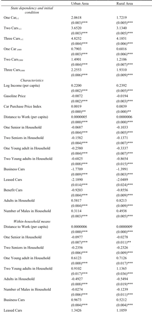
In Table 6 we present our two estimated models, for urban and rural households. One
unexpected estimate is that the car purchase price index is positive and significantly different from zero in both models, which may indicate that this index is a poor representation of car capital costs.
Both the current and permanent disposable income affects car ownership positively. The size of the permanent income effect is larger than the current income effect. The larger effect of the permanent income is also found by Nolan (2010). The long-run effects for a household with at least one young adult (below 25 years of age) or senior household (at least one adult above 66 years) are interesting since they show the dynamics of ageing. Going from a middle-aged to a senior household does not affect car ownership that much compared with the long-run effect of being a senior household. The opposite is found for households with at least one young adult, as the effect is negative in the short run but then becomes positive as they age. The effect of distance to work is significant but very small. The effect of access to a
non-private car has a negative short-run effect but over time the negative effect reduces in size.
In the next section, we will start our analysis of the models using Wooldridge’s (2006) method.
13
Table 6 Regression results for the random effects ordered probit models for urban and rural households
Urban Area Rural Area
State dependency and initial
condition One Cart-1 2.0618 1.7219 (0.003)*** (0.005)*** Two Cars t-1 3.6520 3.1340 (0.003)*** (0.005)*** Three Cars t-1 4.8252 4.1851 (0.004)*** (0.006)*** One Car 1999 0.7903 0.6016 (0.003)*** (0.006)*** Two Cars1999 1.4901 1.2106 (0.004)*** (0.007)*** Three Cars1999 2.2553 1.9310 (0.006)*** (0.009)*** Characteristics
Log Income (per capita) 0.2200 0.2392 (0.002)*** (0.005)*** Gasoline Price -0.0072 -0.0194 (0.002)*** (0.003)*** Car Purchase Price Index 0.0019 0.0039 (0.000)** (0.000)** Distance to Work (per capita) 0.0000005 0.0000006 (0.000)*** (0.000)*** One Senior in Household -0.0687 -0.1033 (0.004)*** (0.005)*** Two Seniors in Household -0.1582 -0.1371 (0.004)*** (0.007)*** One Young adult in Household -0.2580 -0.3337 (0.004)*** (0.007)*** Two Young adults in Household -0.6825 -0.8654 (0.008)*** (0.015)*** Business Cars -1.7709 -1.3991 (0.009)*** (0.003)*** Leased Cars -2.1890 -2.0489 (0.014)*** (0.024)*** Benefit Cars -0.9203 -0.8556 (0.004)*** (0.009)*** Adults in Household 0.5817 0.8213 (0.004)*** (0.009)*** Number of Males in Household 0.3114 0.4938 (0.003)*** (0.005)***
Within-household means
Distance to Work (per capita) 0.0000006 0.0000009 (0.000)*** (0.000)*** One Senior in Household -0.0977 -0.0278 (0.007)*** (0.011)** Two Seniors in Household -0.2356 -0.2326 (0.006)*** (0.009)*** One Young adult in Household 0.6123 0.7126 (0.008)*** (0.017)*** Two Young adults in Household 0.9102 1.1365 (0.017)*** (0.036)*** Adults in Household -0.4927 -0.5494 (0.008)*** (0.019)*** Number of Males in Household -0.0274 -0.1239 (0.006)*** (0.011)*** Business Cars 0.9673 0.5212 (0.004)*** (0.004)*** Leased Cars 1.3426 1.1059
14
(0.029)*** (0.064)*** Benefit Cars 0.2040 0.0380 (0.006)*** (0.013)** Log Income (per capita) 0.1590 0.0265 (0.004)*** (0.007)*** Cut points Cut point1 5.9743 4.8205 (0.051)*** (0.095)*** Cut point2 9.7396 8.2382 (0.051)*** (0.096)*** Cut point3 12.1614 10.6016 (0.051)*** (0.096)*** Rho 0.3397 0.3969 (0.000)*** (0.001)***
Time Dummies Yes Yes
Observations 7441410 2814823 Log-Likelihood -3658020.7 -1620080.3 Standard errors presented in parentheses. Significance level presented as: *** significant at 1 % level, ** significant at 5 % level, * significant at 10 % level.
4.1 Urban Households
The probabilities for the four levels of car ownership are represented in the table below as P(0), P(1), P(2), and P(3). We will start the analysis by looking at the base urban household’s transition probabilities of car ownership and then compare them at another level of the disposable income.
Permanent Income
Area Income P(0) P(1) P(2) P(3)
Urban 173,000 173,000 0.010 0.916 0.074 >0.000
The base household seems to be very state dependent with a 91.6 percent probability of continuing to own one car. The household has a 7.4 percent probability to increase car ownership by one more car and a 1.0 percent to cease car ownership.
When varying the urban household yearly income to the upper lower quintile, 126,000 and to the lower upper quintile, 219,000, we see that the state dependence is stable around 91 percent. The low-income households have a 1.4 percentage units larger probability to cease car ownership and a 5.9 percentage units lower likelihood to buy one more car than the base household. The high-income household has the expected reaction, the probability to cease car ownership is 0.8 percent and the likelihood to buy one more car is 8.7 percent. This is an indication that there is a positive income effect on car ownership. A positive income effect is also found by Nolan (2010) and Dargay and Hanly (2007), although their results are not directly comparable to ours. A 90,000 SEK increase in income per capita yields roughly 2 percentage units higher probability of increasing car ownership from one to two cars. From this income analysis, we can see that households are strongly state dependent and that income levels have considerable effects on the probability of changing the level of car ownership. We will now study how urban households differ based on previous car ownership by comparing the base household with households owning no car the previous period and by
15
comparing households owning cars neither in the previous year nor in 1999 with households not owning a car in the previous year but owning a car in 1999.
Area Cars t-1 Cars 1999 P(0) P(1) P(2) P(3) Urban 0 0 0.703 0.297 >0.000 >0.000
Area Cars t-1 Cars 1999 P(0) P(1) P(2) P(3) Urban 0 1 0.399 0.601 >0.000 >0.000
Comparing the probabilities above with the probabilities for the base household, we see that the state dependence is not as high as it is for ownership when not owning a car in the previous period. The state of owning one car in 1999 seems to play a large role for car ownership in the future. The difference in likelihood of owning one car is considerable, with the probability of acquiring one car being 30 percent for households with no previous car ownership and 60 percent for households that owned a car in 1999. The large effect of being a car owner in 1999 suggests that the household’s preferences may be formed by car ownership. Another important aspect is how the ages of household members affect car ownership. We will therefore examine differences in car ownership for households with young, middle-aged and senior members.
Area Young Senior P(0) P(1) P(2) P(3) Urban 0 1 0.0122 0.923 0.065 >0.000
Area Young Senior P(0) P(1) P(2) P(3)
Urban 0 2 0.0154 0.93 0.054 >0.000
Area Young Senior P(0) P(1) P(2) P(3) Urban 1 0 0.0197 0.936 0.044 >0.000
Area Young Senior P(0) P(1) P(2) P(3)
Urban 2 0 0.059 0.932 0.017 >0.000
Our results indicate that if at least one of two adults in a base urban household is younger than 25 or older than 66 years, it will impact car ownership negatively, increasing the likelihood of the household ceasing car ownership and decreasing the probability of increasing car
ownership. Interestingly, households with senior members do not differ that much from the households with middle-aged members, indicating that they do not exit car ownership a lot more than the base household. The opposite is true for households with two individuals below age 25, which have a larger likelihood of ceasing car ownership and a substantially lower likelihood of increasing car ownership compared with middle-aged households. Our model also reveals that the probability of ceasing car ownership is lower for young adults and higher for seniors over time when looking at the estimated within-household means.
The reaction to changes in gasoline prices are also an important variable for policy makers. It is therefore important to know how it affects a households’ car ownership. It should be noted, however, that our model cannot say whether the driving pattern changes in households but only how car ownership changes.
16
Area Income Gasoline Price P(0) P(1) P(2) P(3) Urban 173,000 13 0.010 0.916 0.074 >0.000
Area Income Gasoline Price P(0) P(1) P(2) P(3) Urban 173,000 16 0.011 0.918 0.071 >0.000
Our model indicates only very small changes in transition probabilities when increasing the gasoline price by around 25 percent for urban households.
A further factor influencing households’ private car ownership is how access to business and benefit cars impacts car ownership. We will compare households with just one private car with households with one private car and one business car and with households with one private and one benefit car, respectively.
Area Income Cars P(0) P(1) P(2) P(3)
Urban 173,000 1 Priv 0.010 0.916 0.074 >0.000
Area Income Cars P(0) P(1) P(2) P(3)
Urban 173,000 1 Priv + 1 Pro 0.068 0.921 0.012 >0.000
Area Income Cars P(0) P(1) P(2) P(3)
Urban 173,000 1 Priv + 1 Ben 0.054 0.93 0.015 >0.000
In households with both a private and a business car, the likelihood of ceasing car ownership is higher and the likelihood of increasing car ownership is lower. Compared with just owning a private car, there is a 4–5 percentage unit higher likelihood of ceasing car ownership and a roughly 6 percentage unit lower probability of increasing car ownership.
Until now we have analyzed households composed of two adults, but our data allows us to analyze households that also include children above 18 years of age. We do not analyze the effect of children below age 18 as we cannot know if they live with one or both parents. We do however look at both the impact of the number of adult individuals in the household as well as the differences between female and male adult children.
Area Males Females P(0) P(1) P(2) P(3)
Urban 1 1 0.010 0.916 0.074 >0.000
Area Males Females P(0) P(1) P(2) P(3)
Urban 2 1 0.004 0.859 0.137 >0.000
Area Males Females P(0) P(1) P(2) P(3)
Urban 1 2 0.008 0.905 0.087 >0.000
Our model shows that there is a difference between households with three adults and households with two. The gender of the adult child is also important. Having a female adult child will only give a slightly lower likelihood of ceasing and a slightly likelihood higher of increasing car ownership compared with the base urban household. A male adult child, on the
17
other hand, has a stronger effect on the likelihood of car ownership, i.e., a 5 percentage unit higher likelihood of owning an additional car than a female adult child.
Our model of “type” households seems to give reasonable explanations to what happens to urban households’ car ownership when altering some key variables. The results indicate a positive income elasticity, large state dependency, some habit effect, an age effect, low gasoline price sensitivity, and an effect of different household compositions. The next step of our analysis is to compare our urban household models with their rural counterparts.
4.2 Rural Households
In this section, we study the changes in transition probabilities in the same way as for urban households using the rural household model’s estimates, and compare the households to look for differences in car ownership transition probabilities between the area types.
Permanent Income
Area Income P(0) P(1) P(2) P(3)
Rural 173,000 173,000 0.0082 0.837 0.154 >0.000
Rural base households have almost twice the likelihood of buying an additional car compared with urban households (15.4 percent vs. 7.4 percent). The probability of ceasing car
ownership is 0.8 percent compared with 1 percent for the base urban household.
The income analysis for urban households revealed a positive income effect on car ownership. We find a similar positive income effect for rural households. Low-income households have a 1 percentage unit higher likelihood of ceasing car ownership and a 13.5 percentage unit lower likelihood of increasing car ownership. The high-income households have a 0.7 percentage units lower likelihood of ceasing car ownership and a 16.9 percentage units higher likelihood of increasing car ownership. The conclusion for the urban households was that income levels have considerable effects on the probability of changing the level of car ownership. A similar conclusion can be made for the rural households, where they have a considerably higher probability of increasing car ownership.
The rural household model exhibits different effects from not having owned a car in the previous year and from not having owned a car for in the initial period long time.
Area Cars t-1 Cars 1999 P(0) P(1) P(2) P(3) Rural 0 0 0.468 0.530 >0.000 >0.000
Area Cars t-1 Cars 1999 P(0) P(1) P(2) P(3)
Rural 0 1 0.249 0.748 0.003 >0.000
The analysis of previous car ownership using the rural household model indicates less state dependence when not owning a car. The model also indicates that rural households are more likely to increase car ownership than urban households. Similar to the urban results, car ownership in 1999 has a strong influence.
18
Area Young Senior P(0) P(1) P(2) P(3) Rural 0 1 0.0108 0.858 0.131 >0.000
Area Young Senior P(0) P(1) P(2) P(3) Rural 0 2 0.0118 0.864 0.124 >0.000
Area Young Senior P(0) P(1) P(2) P(3) Rural 1 0 0.0194 0.892 0.088 >0.000
Area Young Senior P(0) P(1) P(2) P(3)
Rural 2 0 0.0625 0.908 0.03 >0.000
Rural households with one or two seniors have results similar to households with middle-aged members, with just a bit higher likelihood of ceasing car ownership and a bit lower
probability of increasing car ownership. Unlike seniors, households with young adults are less likely to increase and more likely to decrease car ownership compared with middle-aged households. This is the same pattern as in the urban household’s model. Also similar to the urban household results, the within-household calculations indicate that when young
households grow older the likelihood of decreasing car ownership is lower and the probability of increasing car ownership is higher compared to when they are younger. The seniors see the opposite development when growing older.
We turn now to the effects of higher gasoline prices. The urban household model revealed low gasoline price fuel sensitivity.
Area Income Gasoline Price P(0) P(1) P(2) P(3) Rural 173,000 13 0.008 0.837 0.154 >0.000
Area Income Gasoline Price P(0) P(1) P(2) P(3) Rural 173,000 16 0.01 0.849 0.141 >0.000
Comparing the gasoline price sensitivity of car ownership between rural households and urban households, it turns out that the rural households are a bit more sensitive to gasoline price changes. The likelihood of ceasing car ownership is almost the same, whereas the likelihood of increasing car ownership to two cars is 1.3 percentage units lower, which is an 8 percentage units reduction compared to the 4 percentage units reduction for the urban base household.
In the urban model, we found a strong effect of access to non-private cars on private car ownership.
Area Income Cars P(0) P(1) P(2) P(3)
Rural 173,000 1 Priv 0.008 0.837 0.154 >0,000
Area Income Cars P(0) P(1) P(2) P(3)
Rural 173,000 1 Priv + 1 Pro 0.064 0.907 0.029 >0,000
Area Income Cars P(0) P(1) P(2) P(3)
Rural 173,000 1 Priv + 1 Ben 0.057 0.910 0.033 >0,000
In rural households, access to non-private cars implies a substantially higher likelihood (5–6 percentage units) of ceasing car ownership and a substantially lower likelihood (12–13
19
percentage units) of increasing car ownership. The stronger access form, business car, has a stronger effect than the weaker access form, benefit car.
The last aspect we will analyze is how household composition affects car ownership. Again we do not use information about children below the age of 18. The urban household model indicated that a household consisting of two adults and one male adult child implies a
substantially higher probability of increasing car ownership compared with households with a female adult child. This is true also in rural households even if the difference is smaller.
Area Males Females P(0) P(1) P(2) P(3)
Rural 1 1 0.082 0.837 0.154 >0.000
Area Males Females P(0) P(1) P(2) P(3)
Rural 2 1 0.001 0.646 0.350 0.003
Area Males Females P(0) P(1) P(2) P(3)
Rural 1 2 0.004 0.768 0.227 >0.000
Presence of male children raises the probability of increasing car ownership by almost 20 percentage units; the corresponding figure for female children is just 7 percentage units. Comparing households composed of two and three members yields a larger difference in the rural model than in the urban one.
Our rural household model gives plausible effects on our key variables and is similar in effects to our urban household model. We see a positive income elasticity, large state dependency, habit effects, an age effect, higher gasoline price sensitivity, and a larger effect of different household compositions. The most outstanding differences between our two models are that the rural households are more sensitive to gasoline price increases and increases in the number of adult members, and that they show an overall larger probability of increasing car ownership.
4 Conclusions
This paper can be viewed as a first step to study the effects of socioeconomic and
geographical differences on household car ownership in Sweden. Our uniquely rich dataset opens up for detailed analysis of variations in car ownership between different social groups and geographic areas.
Some of the findings in the present paper covering the period 1999–2008 are parallel to the results from an earlier Swedish car ownership model (Matstoms 2002) for the period 1980– 1995, but some results also go beyond the previous study. The principal extensions compared with earlier modeling of car ownership in Sweden are the recognition of households from register data, the use of a more resolved area coding and the modeling of the number of cars. The household recognition allows for a closer comparison with earlier car ownership studies based on household data. The area coding allows us to distinguish differences in determinants of car ownership in urban and rural areas.
We find that rural households with one car are more likely to increase car ownership and less likely to cease car ownership than their urban counterparts. Rural households without a car are
20
more likely to acquire a car and less likely to continue not owning a car than are urban households.
Like earlier studies, we also find that car ownership is very persistent. The results suggest that the state dependence (in the form of lagged car ownership) has a dominant effect on current car ownership. Even the state of owning one car in 1999 has a strong influence on current car ownership. The persistence effect accounts for more than roughly 60 percent of the
probability that a household continues to own a car. For an urban household with median disposable income per capita and no previous car ownership, the predicted likelihood of continued non-ownership is more than 70 percent; for rural households the number is closer to 50 percent. If on the other hand the urban household does own a car, the likelihood of
continued ownership is over 91 percent; for rural households it is 83 percent. This finding is parallel to the findings from the earlier studies. The present study indicates that the urban households have higher state dependence than rural households, whereas rural households have a higher likelihood of increasing car ownership.
The results on exit from and entry to car ownership are also parallel to the results for
individuals. In a companion paper on individual car ownership (Pyddoke and Creutzer 2013), we show that individual men are less likely than women to cease car ownership and more likely to acquire a car if they do not have one. Men are also more likely to increase car ownership than women.
For young men (18-24), Matstoms (2002) finds that they had the largest propensity to acquire a car if they did not have one. This propensity dropped, however, during the 1990s, and in the present study we find a lower propensity to acquire a car for households with at least one young adult than among middle-aged households. The propensities to cease car ownership for households with at least one senior are much lower than for household containing younger adults.
Disposable income per capita is estimated to have a significant positive effect on car ownership for all households. The within-household disposable income per capita or the permanent income has a larger impact than the current disposable income. This is consistent with the positive income effect that Nolan (2010) finds for Ireland and Dargay and Hanly (2007) find for the UK.
In our household models, we get the expected negative relationship between gasoline prices and car ownership. This relationship is the opposite of that in our models of individuals. The effect of a gasoline price increase is not very strong for urban households. Rural household car ownership is more affected by changes in gasoline prices. Note that in this paper, we only analyze car ownership and cannot say anything about car usage.
Our results indicate that the number of children over age 18 has a considerable effect on car ownership. The gender of the child(ren) over 18 also proved to be important, where a male child has a stronger positive effect on car ownership than a female child.
The model used expands the detail with which we can describe the sensitivity of household and individual car ownership to changes in costs and disposable income, as well as its
dependence on gender and type of residence area. The model could be applied to various parts of the population or geographic regions that may be in need of further analysis.
21
Finally, a deeper, more thorough analysis of households that cease car ownership could possibly shed more light on further causes of termination of car ownership, like moving, job loss, and loss of disposable income.
Acknowledgements
We are grateful to Sherzod Yarmukhamedov for several valuable suggestions and to the participants at a seminar at VTI on September 6, 2013. We also wish to thank Urban
Björketun, who did most of the work on collecting and correcting the data and who did all the estimations for the previous paper (Pyddoke 2009). We also want to thank Emma Robert Freijinger for bringing to our attention that cars owned by proprietary firms were included in the data that was supposed to contain only privately owned cars.
References
Akay, A., 2009. The Wooldridge Method for the Initial Values Problem Is Simple: What About Performance?, IZA Discussion Papers 3943.
Dargay, J., Hanly, M., 2000a. Car ownership in Great Britain: a panel data analysis, Transportation Research Record, 1718, Activity Pattern Analysis and Exploration, Travel Behavior Analysis and Modeling, 83-9.
Dargay, J., Hanly, M., 2000b. Car ownership in Great Britain: a panel data analysis, European Transport Conference, September 2000, Cambridge, TSU Ref 2000/17.
Dargay, J., Hanly, M., 2007. Volatility of car ownership, commuting mode and time in the UK, Transportation Research A, 41, 934-948.
Dargay, J., Vythoulkas, P., 1999. Estimation of dynamic car ownership model: a pseudo-panel approach. Journal of Transport Economics and Policy 33 (3), 283–302.
de Jong, G.C., Fox, J., Daly, A., Pieters, M., Smit, R., 2004. Comparison of car ownership models. Transport Reviews 24 (4), 379–408.
Jonsson L. and Freijinger E., 2012, Validation of the Swedish national car ownership model, (in Swedish), report to the Swedish Transport Administration.
Kitamura, R., Bunch, D.S., 1990. Heterogeneity and state dependence in household car ownership: a panel analysis using ordered response probit models with error components. In: Koshi, M. (Ed.), Transportation and Traffic Theory. Elsevier Science Publishing Co.,
Amsterdam.
Matstoms, P., 2002. Modeller och prognoser för arealt bilinnehav i Sverige. VTI rapport 476. Nolan, A., 2010. A dynamic analysis of household car ownership. Transportation Research Part A: Policy and Practice 44 (6), 446–455.
Pyddoke, R., 2009, Empirical analysis of car ownership and car use in Sweden, VTI rapport 653.
22
Pyddoke and Creutzer, 2013, Individual car ownership in urban and rural areas in Sweden 1999-2008, working paper.
Vagland, Å. and Pyddoke, R., 2006, How households adapt to changed costs for car ownership and car use, (in Swedish), VTI rapport 545.
Wooldridge, J., 2005. Simple solutions to the initial conditions problem in dynamic, nonlinear panel data models with unobserved heterogeneity. Journal of Applied Econometrics 20 (1), 39–54.
Wooldridge, J., 2006. Introductory Econometrics – A modern approach, Thomson-South Western.
23
Variable list:
Individual: Age, Gender, Children, Disposable income of individual, Place of residence, Area type of residence, Distance to workplace, Number of cars owned by individual, Number of employer supplied cars: business and benefit.
Household: Number of adults, Age, Gender, Disposable income of adult members of household, Disposable income per adult household member (average per adult), Average permanent disposable income of household.