The Impact of Inflation on Capital Rotation in Inflationary Inflection Points : An Investigation on How Inflation Affects Capital Rotation Between Major Market Sectors as Economies Shift from Disinflation to Reflation

(1)

The Impact of Inflation on Capital Rotation in

Inflationary Inflection Points

An Investigation on How Inflation Affects Capital Rotation Between

Major Market Sectors as Economies Shift from Disinflation to Reflation

(2)

Bachelor Thesis in Economics

Title: Impact of Inflation on Capital Rotation in Inflationary Inflection Points. Authors: Lukas Berzups & Philip Hansson

Tutor: Rafael B. De Rezende Date: May 2021

Key terms: Inflation, Inflation Cycles, Reflation, Rising Inflation, Decreasing Inflation, Disinflation,

Capital Rotation, Capital Cycles, Inflection points, Interest Rates

Abstract

There has been a multi-decade disinflationary period that, with the conjunction of recent pandemic-related events, led to extremes in various economic metrics: record lowest interest rates and inflation, increasingly loose monetary and fiscal policies leading to severe debt levels and money supply - all resulting in a multi-front pressure on inflation to start increasing, and after 30 years, for economic environments to reach an inflection point from disinflation to reflation. How would various market sectors perform if suddenly inflation starts to surge? Previous research of similar events, such as in the 1970s, as well as theory, points towards certain market sectors and asset classes, such as commodities, to outperform their peers. Research on this topic is fairly scarce, thus, to better prepare for such an inflationary event and gain insight on which market sectors are best to invest in or avoid, this paper conducts an investigation to explore that scenario. By looking at 11 major market sectors over 10 countries' historic inflationary points that shifted from disinflation to reflation, analysis determined that, while certain sectors are indeed more sensitive to changes in inflation than others, many more are sensitive to changes in interest rates that normally accompany inflation. Sectors such as Energy, Consumer Discretionary and Financials would perform well during this period, while sectors such as Information Technology would historically underperform. Contrary to the theory, not enough relation was discovered by the analysis towards the commodity sector as a whole to overperform, however, that does not mean that none exist. Further research is still required on this topic to increase knowledge and awareness so that the negative impact of inflationary events like the ones of the 1930s and 1970s can be avoided and even taken advantage of.

(3)

1. Introduction

Inflation is a subject that is rarely fully understood or prepared for. While small amounts can help benefit and stimulate economic expansion, once it is let loose and the control is lost, it can destroy countries and societies. Big fluctuations can bring incredible rewards to the prepared, while severely punishing the ones who are not. At the core, low or high, inflation is the decay of money, and it benefits the ones with high debts and punishes the ones with high savings. It rewards the indebted speculator, the greedy company with leveraged balance sheets, and the fiscally irresponsible governments, all at the expense of the conservative saver or ordinary person. High inflation is a very severe risk event, during which there is much stress on the companies and individuals. In the last 1970s inflation crisis that hit the developed world, unemployment rates skyrocketed, stock markets lost about half their value in a short time frame and interest rates rose to over 20%. Countries that experience high inflation become politically and socially destabilized, granting an opportunity for political extremists to gain popularity caused by anger and suffering of the general public. As history suggests, a lot of the worst historic events followed periods of high inflation.

Many countries have focused on using loose monetary policies that aim to lower the inflationary pressure in order to meet targets and control big debt levels. The FED in the US has long tried to battle the pressures of inflation - rising inflation used to be a worry up until 2008, when the US instead of focusing on preventing a recession(Amadeo, 2021), pumped several trillion dollars in an effort to keep banks solvent. This led to worries that the economy would see inflationary pressures arise, but the US has, up until recently, managed to hold its official target of 2% yearly inflation. As of now, the US and other countries have been forced to provide extensive stimulus packages once again to mitigate the impact of Covid-19 on the population, however these attempts of preventing recession led to even greater inflationary pressures, and just like dropping Mentos into a Coke bottle, there is a limit until when it will burst with compounded force.

Inflationary effects could be impacting the world as we move forward. Due to the Covid-19 pandemic, economies and businesses started suffering and drastic measures have been taken in order to prevent a recession. In 2020, the US injected 9 trillion dollars into the market, 22 % of that was printed, increasing the total money supply (Cage, 2021). However, due to these measures, major economies avoided crashing further down and recovered quickly in March 2020. These pumps have led to a devaluation of the USD, nevertheless, with little impact seen on the economy.

As a result of the 1.9 Trillion Dollar stimulus package and economies opening up as the Covid-19 vaccines get distributed, economists have started raising their inflation expectations as seen through a survey done by the wall street journal - a 2.48% increase in inflation in December compared to the prior year (Kate Davidson, 2021). Many other economists such as Andrew Hunter have said in the previous year that higher inflation rates should be expected to start picking up in 2021 since the demand for goods and services will start rising once Covid-19 eases up and the supply will be limited (Cox, 2021). Big banks, such as Morgan Stanley, predict higher estimates of growth than the FED, stating that a big factor is the return of inflation(Golubova, 2021). Monetary policy will respond to the rise in inflation by raising real interest rates, which will cause an increase in the marginal cost of business. This in turn will add to high inflationary pressures on business profits and further disincentivize investments due to the multi-front pressure of high inflation and interest rates on businesses (Parmenov & Moullé-Berteaux, 2020).

According to the theory of Inflation Cycles, the current economic environment points towards a transition between Phase 1 - “Pre-Inflationary Period” and Phase 2 - “Inflation Shock/Surge”: High fiscal deficits with loose monetary policies, sharply rising equity markets, artificially low-interest rates, and vast amounts of credit available at those low-interest rates. This stage comes in the form of an inflationary shock, catching many people off guard. It predicts that the rising inflation will cause interest rates to increase rapidly, causing a fall in equity markets, liquidity to be channeled into real assets such as commodities, and economies to fall into a recession (H. Hammes, 2016).

(5)

Debt Cycle and Capital Cycle theories further reinforce the upcoming path described by the Inflation Cycle theory. Ray Dalio (2017) argues that a low-interest rate environment causes increased spending and therefore more revenue to spend for businesses and income to consumers. Increased spending results in a higher demand for goods and services inevitably leads to an increase in inflation until there is a higher response in the interest rates. This increased capital flow originated from low-interest rates, according to Edward Chancellor (2015), will lead to lower returns on newly invested capital. Once the returns drop to a certain point, capital will flee the sectors until it becomes sufficiently attractive again, just like it happened in the 2000 Tech bubble and 2008 mortgage crisis.

This study analyzed 11 major market sectors performances in over 10 countries. By analyzing how market sectors perform in relation to inflation and interest rates, the results confirmed the close relationship between interest rates and inflation, however, it showed that, at a reflationary period, most market sectors are more affected by the change in interest rates than fluctuations in inflation. Not all terms of interest rates were affecting market sectors equally, some sectors seemed to be more sensitive to change in the short-term rates, while others more towards long-term rates. Contrary to the theory, the majority of the commodity-based sector's performance could not be explained by inflation or interest rates in this study. Based on the gathered data, there were several sectors that showed great sensitivity to inflation or interest rates. Those sectors were Financials, Information Technology, Consumer Discretionary, Telecommunications, Utilities and Energy.

There were several prior studies and publications related to this topic. The most comparable one was done by Schroders Asset Management Company (2014): It analyzed the performance of the Energy and Materials sectors during the 1970s inflationary period, revealing high overperformance of the commodity sectors. Research on volatility caused by macroeconomic factors such as inflation was done by Geske and Roll (1983) and Soenen and Hennigar (1988), but the results were inconclusive on the connection between inflation and market performance, as both positive and negative connections were found. Another study in search of a good hedge against inflation was done by Bethlehem (1972), where a selection of industrial-related equities in South Africa proved to be a good approach. Not all research points toward the same direction as Bakshi and Chen (1996), which showcased a negative correlation between inflation and stock prices, though.

How and if capital rotates between different sectors as we move from one inflationary environment to another, seems to be an under-researched topic with no clear consensus and analysis on all the sectors. Seeing as we are now in a historically low and decreasing inflationary environment that can pivot at any point, the importance of understanding its future effects and being prepared for them has never been more relevant in this century. Capital rotation1_{analysis can be used as a strategy to find out what} the best performing sectors are and discover insights towards the implications it has on different businesses alongside inflation.

Unlike other research that primarily look at how inflation affects economies as a whole, this study aims to find out how major market sectors are affected when an economy goes from a disinflationary2 environment into a reflationary3_{environment. It will observe and reference back to theory any capital} movement between these environments while looking at potential causes for these movements to occur. The paper will try to add insight and provide a discussion by analyzing what has happened with the capital in economies during similar historic inflection4_{points. Exploring if capital movement} between major market sectors is caused by inflation, what the underlying trends are and what the theoretical reasons could be that is causing these trends to occur. Results might aid an entity or

(6)

2. The Inflationary Tide

2.1 The Great Inflation of the 1970s

From the mid-1940s the United States was in a disinflationary trend and experienced very

low-interest rates and inflation until between the mid-1950s to mid-1960s. This low inflation period was fueled by loose monetary policies and growing budget deficits supported by political leaders. All that resulted in what is now referred to as the 1970s Great Inflation, during which ever-rising inflation in the form of three waves hit the unprepared economy. This phenomenon lasted a decade.

Graph 1: US National Debt Compared to GDP & Fed Fund Rate 1947-1980 adapted from https://www.thebalance.com/national-debt-by-year-compared-to-gdp-and-major-events-3306287 (Appendix Graph A1)

Looking at the historic Buffet Indicator (Graph 2), which is market value to GDP ratio, market participants enjoyed extreme returns through the disinflationary period until the end of the 1960s when the markets reached extreme overvaluations with close to two standard deviations from the historic trend.

(7)

These valuations were not sustainable and once inflation and interest rates started to rise and the economy shifted from disinflationary to a reflationary environment, the market value dropped by almost 50% over a 20 month period, unemployment reached double digits and the increasingly harder access to capital caused many businesses to fail.

Schroders Asset Management Company (2014) in one of their yearly “Investment Perspective” publications called “What are the inflation beating asset classes?” did deep research into the performance of various sectors across the 1970s. They discovered that while inflation brought negative equity returns for the S&P Index as a whole, material-related equities remained mostly constant and energy equities thrived throughout the whole cycle.

Graph 3: Energy equities data from the Federal Reserve Bank of St Louis

Similar results of commodity-related sectors having strong outperformance during the decade can be seen in a showcased study by Longview Economics (2021). In the analysis, even commodities with a reduced energy rating, outclassed the rest of the market sectors throughout the 1970s (Graph 4).

(8)

This is further confirmed with an analysis made by the BofA Global Research (2021) on 10 years annualized returns of commodities, showcasing the overperformance throughout the 1970s (Graph 5).

Graph 5: Commodities rolling return from BofA Global Equity Strategy, Global Financial Data, Bloomberg

At the end of that decade, depending on the positioning and preparedness of the investor, he could have reaped fruits of generational wealth or accumulated immense loss requiring several decades to recoup.

(9)

2.2 Is the stage set?

The United States economy has been in a decreasing inflation environment ever since the 1970s, which has been the most prolonged disinflation period in modern history, lasting for over 30 years. Now the period is being stretched by loosening monetary policies, substantial budget deficits, and historically low interest rates (Graph 6).

Graph 6: US National Debt Compared to GDP & Fed Fund Rate 1950-2020 adapted from

https://www.thebalance.com/national-debt-by-year-compared-to-gdp-and-major-events-3306287(Appendix Graph A2)

For the past decade inflation and interest rates barely went above 2.5%, while to sustain such low rates, the budget deficit and money supply have skyrocketed (Graph 6).

Only in 2020 total money supply M1 (cash and checking deposits) increased by over 60% of the total existing money supply (Graph 7).

(10)

High central bank liquidity and decreasing interest rates created the perfect environment for the growth stocks to thrive as visualised in the study done by BofA Global Investment Strategy (2021) (Graph 8).

Graph 8: Central Bank Liquidity and Market Capitalization from BofA Global Investment Strategy, Bloomberg

The current economic environment has discouraged savings, encouraged consumer spending, and incentivized large funds to take on more risk to meet harder to reach return targets. Easily accessible money has, in turn, caused higher demand for certain goods, raising their prices. A change in the current low rate bond market norm could lead to an increase in the cost of capital and make it more expensive for businesses to grow or even maintain the current market capitalization. The increased cost of operation could eventually reflect into the final cost of consumer goods, bringing further pressure towards inflation.

In many ways, the economy is now resembling how it was back in the 1960s, and even the commodity sector has historically underperformed compared to other sectors, just like before the Great Inflation Graph 4 and 5) afterwards resulting in a commodity supercycle. Does that mean that the stage is getting set for an encore with inflation leading the way? With extremes across various metrics and a multi-front pressure on inflation, it may be beneficial to be aware of the risks and be prepared for a potential disinflationary inflection point towards a sustained reflationary period, just how it was observed in the 1930s and 1970s. As Mark Twain said, history does not repeat itself, but often rhymes - there may be differences in how things unfold, but in the end, it can lead to a similar result. Thus while it would be very hard or nearly impossible to forecast when and if inflation might increase, it could be very beneficial in preparation for such an event to analyse how different sectors perform during such inflection periods, how capital might be rotating between those sectors and which ones would be best to be positioned in.

(11)

3. Theoretical Framework

3.1 Inflation Cycles

In his recent release of “Return of High Inflation”, Wolfgang argues that excessive accumulation of debt and the monetary strategies that have been put in place to accommodate the economy over the last three decades will be the main drivers for a return of high inflation.

(H. Hammes, 2016) segregates the sources of inflationary pressures into two categories -demand-driven inflation and loss of faith-driven inflation. The -demand-driven inflation is caused by increasing demand for goods due to the Industrial revolution in emerging markets, world economic growth, or population-rich emerging markets becoming global consumers. Loss of faith-driven inflation is driven by market participants losing faith in paper money, high fiscal deficits, and government debts with loose expansionary monetary policies. He further breaks down the loss of faith-driven inflation into three steps. The first step being prolonged fiscal deficits, high government debt, and expansionary monetary policy. In the second step companies and individuals have significant cash and there are high liquidity volumes. Which finally results in loss of faith in paper money, bubbles in equity and bonds bursts, flight into (real) assets, and “stable” currencies.

Wolfgang (2016) introduces the 5 phases of the inflationary cycle and identifies these as the most critical to be the initial transition between low to high inflation as high inflation dramatically changes the rules for the economy, finance, and business management.

Phase 1 is described as a pre-inflationary phase of economic strength and prosperity. An example period between 1970 and 1972 is discussed, where the U.S. stock market reached new highs and the economy grew strong during the beginning of the new inflationary cycle with a euphoric mood spreading among companies and investors. All with little realization that unsustainable fiscal, monetary, or economic policies are the leading causes for temporary economic and financial prosperity (H. Hammes, 2016).

The inflation shock (Phase 2) problem unfolds abruptly and fast. Accelerating inflation rates catch the majority of people unprepared. During this phase, business and economic conditions change dramatically: banks tighten credit policies for everyone, interest rates increase rapidly, and the economy is likely to suffer a recession (H. Hammes, 2016).

Eventually, in Phase 3, inflation starts to level off, creating an opening for companies to prepare for the final phase of disinflation, where economic conditions will be changing dramatically, requiring

(12)

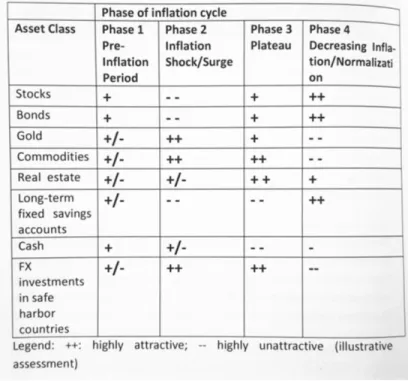
(H. Hammes, 2016)summarizes the characteristics of each Phase in the below table:

Table 1: Phases of the Inflationary Cycle from “Return of High Inflation” Wolfgang (2016)

Lastly, Wolfgang (2016) provides an analysis of various asset classes' historical performance during various phases of inflation. Where he summarizes that stocks and bonds mostly perform exceptionally during a decreasing inflation environment, where businesses benefit from low-interest rates. Gold, commodities, and Real Estate should benefit mostly during the surge and stabilization phases of inflation, providing a safe harbor from inflation. Long-term fixed saving accounts should benefit only in a disinflation environment, where high-interest rates are locked in before the rates start to drop.

(13)

3.2 Debt Cycles

Ray Dalio (2017) and one of the most successful hedge funds of all times, Bridgewater, have published “How the Economic Machine Works'', where they have showcased the Debt Cycle model that follows a logical progression of economic sequences created by the structure of the monetary system. In the model, they describe the effects of interest rates and their impact on the fluctuating demand for credit, which can push both short-term business cycles lasting less than 10 years or cause long-term secular cycles lasting multiple decades.

The process can be summarized in 6 steps:

1. Decreasing interest rates by central banks resulting in a lesser cost of money and lending rates 2. Borrowing becomes cheaper, enticing consumers and business to spend and borrow more (an

increase of demand)

3. Existing debt becomes cheaper to service, resulting in consumers and business with more income to spend (an increase of demand)

4. The discount rate that financial assets and businesses get valued at decreases, causing an increase of the present value of assets, causing a shift into riskier assets (an increase of demand)

5. As one person’s spending is another’s income, an effect of increasing wealth and improving credit profiles is created, allowing consumers/business to borrow and spend more, which causes a virtuous demand cycle.

6. The process would go until rising demand reaches the limits of productive capacity of an economy. When that happens demand-pull inflation begins to accelerate as there is more demand than what suppliers can handle. Once that happens, central banks are forced to raise interest rates, causing the feedback loop to shift into reverse, until the interest rates are decreased again and the cycle starts again (Dalio,2017).

A short-term debt cycle repeats over time; with every repeat, interest rates have to reach new lows due to increasing debt and associated cost of serving it in private and public sectors, data visualisation in Graph A3 within the Appendix. Examples of this can be seen in 1999 and 2000 where the Fed raised interest rates in the US until demand and asset prices started to fall and the economy went into recession after which to counteract, the Fed was forced to lower from almost 7% to 1%. The cycle repeated between 2004 and 2007, where the interest rates were raised to over 5%, until 2008 where the Fed had to combat the recession and lower the interest rates to 0.14%, dropping to a new secular low (Dalio, 2017).

When the rates cannot be lowered anymore (when they reach zero or negative), a pivot in the

long-term debt cycle occurs. This happens because debt levels cannot go to infinity and interest rates

cannot be lowered further to keep everything going. Zero bound is reached and there is no amount of credit easing that can induce people to borrow and spend more as the accumulated debt becomes too high and servicing costs too large. These pivot points usually happen once every generation, around every 25-50 years, and take decades to unfold. In 1920 interest rates were at 5% and decreased to less than 3%, during which the debt to GDP went from 150% to 260%. To service the increasingly high debt, interest rates had to reach new lows of 2% and kept low until the debt was reduced to less than 150% in 1950. Thereafter trending higher for the next 40 years, peaking in 1981 at over 15%, trending down ever since with Debt to GDP increasing to over 380% (Dalio, 2017). Long- Term debt cycle illustrated in Graph A4 within the Appendix.

(14)

3.3 Capital Cycles

The Debt Cycle model looks at the economy from a demand perspective, however, this can be done from the supply side. The debt cycles’ effects on the supply side are described by Edward Chancellor’s “Capital Cycle” approach, in his book “Capital Returns”.

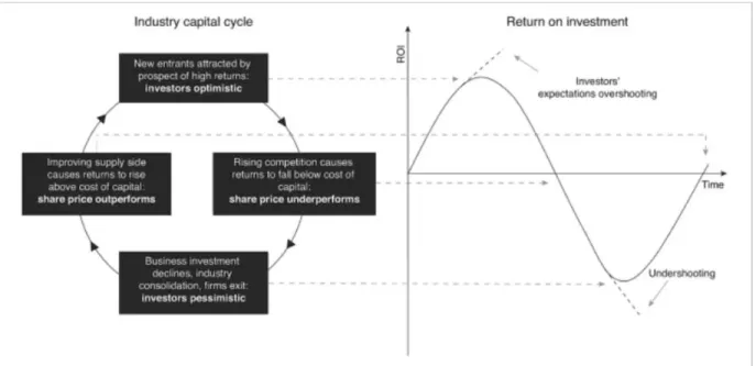
Chancellor (2015) argues that capital is drawn towards businesses having higher returns and flees when the returns fall below the cost of capital. When the capital flows in, new investments, higher competition, and higher capacity emerge. An increase in capacity will lead to lower returns on the capital being invested. Once the returns drop below the cost of capital, capital will flee causing capacity to decrease, this will continue until profitability is back. The cycle can be seen in the illustration below (pp,4-13).

Figure 2: Industry capital cycle and Investment Returns from “Capital Returns” Chancellor (2015)

One example is in the 1990s during the tech bubble when there was a telecommunications bubble. As blind capital was flowing into the tech sector, telecom companies started to increase and double their fiber cable infrastructure every three months, which in fact was double the growth rate of their traffic. The excessive supply caused the telecom industry to severely crash in 2001, after which investment left the sector, which caused it to slowly outperform in the following years due to demand catching up, yet the infrastructure supply was limited (Chancellor, 2015).

Similar scenario happened with real estate during the housing bubble, during which the home prices to income reached extreme levels. Rising real estate prices resulted in overinvestment and excess supply of capital, until the cost of capital was too high for the returns, causing the capital to flee (Chancellor, 2015).

The Debt Cycle model and Capital Cycle model are different sides of the same coin. Both Chancellor (2015) and Dalio (2016) agree through the models that the longer interest rates remain suppressed the more investors will tend to seek out riskier investments. The Debt cycle allows seeing how the cycle starts and how decreasing interest rates kicks off capital’s search for investment, which leads to higher capacity, causing lower returns. Once the pivot point is reached at the end of the business cycle, increasing interest rates lowers the demand and raises the cost of capital, while according to capital theory, future returns decline due to overcapacity. As demand decreases and supply increases, an extreme positive sentiment leads the cost of capital much more than the actual return of capital. right until no more debt can be taken and the start of a new secular trend (Chancellor, 2015).

(15)

3.4 Inflationary Pressures Due to Demographic Reversal

Goodhart & Pradhan (2020) argue in their book “The Great Demographic Reversal” that currently the ongoing disinflationary spiral and expectations for low inflation are not sustainable and a shift towards high inflation will happen in the foreseeable future. They do so by looking at major trends that are reshaping global society and economy, deriving 3 reasons for inflation to increase.

1) World's population is aging due to the declining global birth rates and increasing age at which people get married and have children. This increases the expenditures towards dependents, such as health and elderly care. Simultaneously the dependency ratio will weaken as the number of dependents will be increasing much more than the production population. This will stimulate consumption and decrease production as dependents will be consuming without producing. Aging population trends have been already visible in the US and Europe, however, it starts to appear in China as well, magnified by their previous decade-long 1 child policies.

2) Due to the decreasing dependency ratio, the amount of productive labor will be decreasing, causing limited supply of labor and an increase in its bargaining power in relation to capital. This will lead to inflationary pressures on wages to increase.

3) Decrease in savings and increase in spending due to elderly using their pensions and savings towards consumption with minimal income. Consumption for public expenditures such as care-related costs will be driven up (Goodhart & Pradhan, 2020).

(16)

4. Methodology

To analyze the impact inflationary environments have had on the different major economic sectors a regression is conducted. This will be done on three major economies' entire historical data, to determine if we can see a long-term connection between inflation and sector performance. This is done to see the sensitivity of stock returns towards inflation. Secondly, regression will be conducted on several combined periods based on inflection points, taking samples of the entire population data to determine if the independent variables have any effect during these time periods in general throughout markets. This is done on data sets where the economy which is in a period of disinflation changes into a period of reflation. Since the study consists of several different types of data that can be addressed in several different ways, the paper will analyze and interpret each regression results separately.

4.1 Dependent Variables

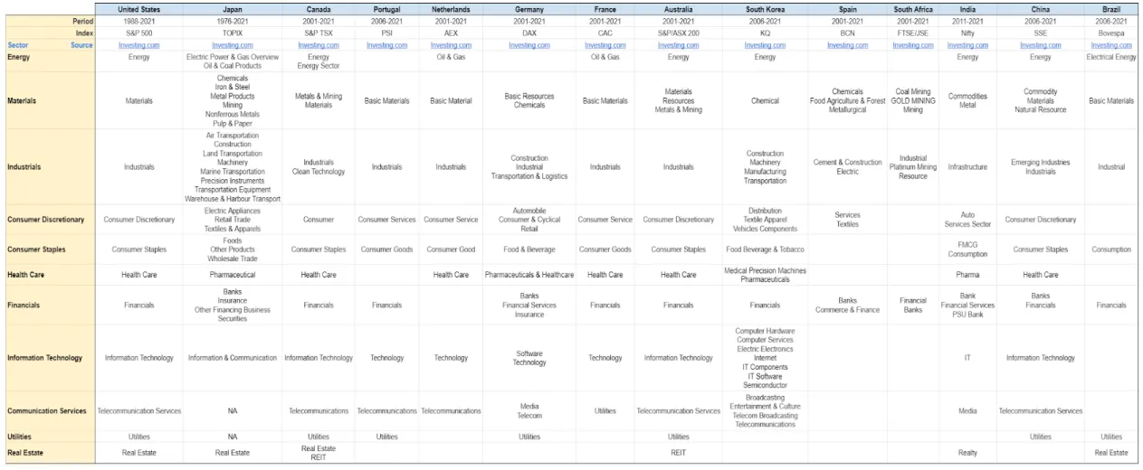
Since the study intends to see if inflation has an impact on capital rotation, it uses market sector performance where various country indices on a yearly basis will be used. The data is gathered from various sources and some indices may have data dating further back than others. A summary of the data used and sources can be found in the table A17 within the appendix.

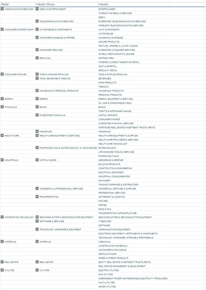
Some countries do not have the standard market sector indices and instead, performance is tracked at an industry or industry group level. In those cases, the indices will be manually categorized into sectors based on the official Global Industry Classification Standard (GICS®) and analyzed in aggregate. In some cases, some countries' full 11 sectors can not be mapped out, in which case a sector with no data for that country would not be included in the aggregate. The details of categorization can be found in the Appendix.

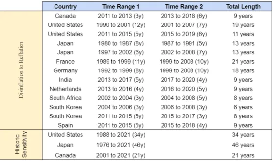
To test historic sensitivity of sectors to inflation, a full range of available data will be taken for countries chosen with the most data. However, when testing the sensitivity of market sectors at the shifting points of disinflationary to reflationary or reflationary to disinflationary, time ranges will be manually selected with a criteria of at least 3 years in both of the directions of the inflection point of continuously increasing or decreasing inflation.

(17)

To be able to compare the performance of different market sectors from various countries, a percentage performance will be used instead of an absolute amount, making the coefficients of the independent variables comparable. The Year on Year variance was calculated by taking the absolute value from the current year - the absolute value from the previous year divided by the absolute value of the previous year. The formula used can be seen below.

ΔRETURN

= (

VALUE_t

-

VALUE_{t - 1}

) /

VALUE_{t - 1}

4.2 Independent Variables

The study has chosen to limit control variables to inflation and interest rates as those were the foundational pillars applying to all economies described in the theory. As there could be multitude of factors, which could be sector or country specific, narrowing down on specific variables is done to prevent fishing for significance.

4.2.1 Inflation

Within the study, the interest rate used is the historical inflation rate based upon the Consumer Price Index (CPI). The constraint of using CPI to measure inflation relative to market performance is that CPI is a responsive measure and may take some time to reflect the real-world inflation, to which there would have already been an impact on the economy. Due to that, the model introduces a forwarded inflation to take into account that businesses act before the inflation rate changes, thus the sector’s performance might have already taken the coming inflation into account. This is assumed within the thesis to be similar to expectations. The future inflation rate is the inflation rate of the time period minus one (i.e. 2011 inflation would be paired with 2010 data). The data is gathered on a monthly and yearly basis, however, yearly data will be used unless otherwise specified. The two variables will be denoted as Inflation and Inflation+1 for future inflation. Details of inflation data can be seen within table A18 in the Appendix.

4.2.2 Interest Rate

Interest rates are in accordance with data provided under the theoretical framework, that pointed towards an impact on certain sector’s performance due to affecting cost and access of capital, as well as debt refinancing. Theory also proved them to be closely linked to inflation as, when inflation increases, interest rates need to increase as well to offer a positive inflation-adjusted return. Including interest rates in the model might give additional pointers on how capital might rotate between sectors. Interest rate data will be based on 2, 10, and 30-year bond yield rates to represent short-term, medium-term and long-term rates. This is done because interest rates throughout various time spans have different volatility, which according to theory may lead some sectors to be more sensitive to a shift of a specific time frame than others. Full details of interest rates can be seen in table A19 within the Appendix.

(18)

4.3 Determination of Inflationary Environment

Disinflation refers to the fact that the economy is in an environment where the pace of inflation is decreasing, meaning that there are lower inflation rates year after year. When the pace starts to increase again, the economy enters a reflationary environment with the inflation pace increasing year after year. Between these two environments is the point of change - the inflection point. These periods are not limited by time and so they can vary in length. For example, in the graph below the US and Japan’s inflation rate is depicted over time, during the period of 2009 we have an inflection point, which in prior to this we had a disinflationary environment and afterwards a reflationary environment. When choosing the inflection points a criteria of at least 3 years in either direction was deemed required, both to have a large enough sample due to yearly data points and to fit within the short-term debt cycles described by Ray Dalio. The process of choosing is visualised in Graph A7 in the Appendix.

4.4 Econometric Model

The time series analysis covers two different types of data, defined within the thesis as “sets”. The first set will be tested using Model 1 to test entire countries’ historic sector sensitivity to inflation in order to determine if there is a long-term effect on changes within sector’s performances on a yearly basis. Model 2 will be used on the second data set, when an economy moves from a disinflation to reflation. Model 2 data set will be split into two parts - sets 2 and 3. The details of the time frames and how they were picked and defined is found under the methodology section. Also since there are different types of interest and inflation, model 2 is a hybrid version in which we primarily use the inflation rate and 10-year interest, but also the future inflation and the three different types of interest rates. This is done since inflation could be seen as sticky and decisions might have already been done based on the future years inflation rates. Also, the reason for the testing being done separately is to avoid multicollinearity within the model, which would provide us with erroneous results.

The goal of the study is to measure if any signs of capital rotation caused by inflation can be seen in historical data or at handpicked inflection points. A significant independent variable would be a sign that during these periods there would be a significant relation between the dependent and independent variables. This theory proposes that inflation and interest rates affect capital rotation.

Model 1

Δ

DEP

_{t, c, s}

= A +

β

₁

π

_{t, c}

+

є

_{t, c, s}

Model 2

Δ

DEP

_{t, s, e}

= A +

β

₁

π

_{t, e}

+

β

₂

R

_{t, e, i}

+

є

_{t, s, e} Where:

Δ = Year on Year Change in the variable DEP = Yearly returns for the sector analyzed

A = Intercept of the equation

= Coefficients of the independent variables

β

= Yearly inflation rate

Π

R = Yearly interest rate = Error term of the model

𝜖

s = Market sector c = Country t = Time period

e = Inflationary environment (Disinflationary, Reflationary) i = Interest rate term (2/10/30 Year)

(19)

4.5 Plan of Analysis

In order to investigate whether or not the inflection points have an impact on the chosen market indices, the analysis will be done on each of the sets after which the results will be compared to the existing theoretical evidence and checked for any existing relations. The following strategy is used:

1) The first part consisted of selecting the inflection points of interest, the points selected can be seen in the table under the methodology section.

2) In the second part of the analysis the data is tested for a unit root, this is done by running an ADF test created by Dickey and Fuller to avoid a spurious regression.

3) In the third part of the analysis, descriptive statistics and a correlation analysis are run which is used to further give an in-depth view of how inflation generally affects each of the sectors and to determine any underlying potential relations, this is done on set one only.

4) In the fourth part, a linear regression model using OLS is used to test the relations between the variables.

5) Lastly, in the fifth part of our analysis, the regression is checked through the Breusch Godfrey serial correlation LM test and Breusch Pagan Godfrey heteroskedasticity test. The data is also tested for multicollinearity using VIF. The data is already corrected within the regression results.

When looking at multicollinearity variance inflation factor is used where the values are interpreted as >10 having severe multicollinearity Gujarati (1988). This is done only on the multivariable models since multicollinearity implies a relation between the independent variables. Also, researchers have mixed opinions on the maximum values of VIF allowed, (Hair et al., 1995) Hair has in the past stated the max value to be 10 whilst Ringle (Ringle et al., 2015) has stated that VIF of 5 is the maximum allowed value, however both state that it is dependent on the type of research, but a lower VIF value is to be considered as better.

(20)

5. Empirical Model and Results

5.1 United States, Japan and Canada Historic Sensitivity to Inflation Analysis

5.1.1 Overview

Analysis under this section is done to determine the overall historic significance of inflation towards various sectors. The data used is sector performance to date for 3 specific individual countries with the most history of financial data and accurate sector grouping. This analysis is not meant to be done for all countries, but to establish a general sense of underlying historic sector trends to inflation.

5.1.2 Data tests

Data and regression results have gone through several checks in order to ensure that the analysis has a solid foundation.

Before running the data, an Augmented Dickey-Fuller Testing (ADF) test is applied in order to determine if the data is stationary or not to avoid a spurious regression. Due to the purpose of this regression the test has first been conducted at level, followed by a random walk and random walk with a drift. ADF test revealed unit root under Japan's inflation data and Canada's Consumer Staples sector, which got corrected by taking the first difference.

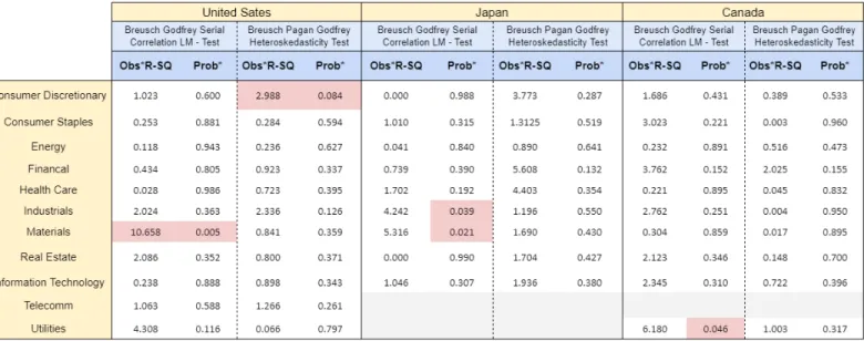
The data was then tested for serial autocorrelation using the Breusch Godfrey LM-Test. Results showed that Materials and Utilities in the United States suffered from serial correlation. To remedy it, Newey-West standard errors were implemented.

Finally, a check for heteroskedasticity was done using the Breusch Pagan Godfrey Test. Few sectors suffered from heteroskedasticity - Consumer Discretionary and Materials in the United States, Industrials and Materials in Japan, Utilities in Canada. To correct the data Huber-White standard errors were implemented.

All the regression results are showing already corrected output. The details for the tests as well as full descriptive statistics summarizing the data can be found in the appendix.

5.1.3 Regression Results

Looking at the regression results, Japan's sectors did not provide any significant results at any level. The p-values for inflation were high and R-squared were very small, implying that the model explained very little of the changes in the dependent variable. Thus it cannot be said that yearly inflation has an impact on any of the sector’s yearly change in performance at any statistically significant levels.

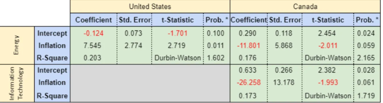
For Canada, the regression revealed that the sectors Consumer Discretionary and Information Technology, showed a significant relation between the independent variable inflation and the dependent variable yearly change in sector performance, P-values being 0.0587 & 0.0609 with coefficients -11.801 & -26.528, Thus indicating that an increase in inflation showed signs of a decrease in the sector’s yearly performance. R-Squares were around 0.17 implying that inflation explained roughly 17 % of the changes in the dependent variable.

In the United States, there was only one sector that showcased a significant relation between the independent variable inflation and the dependent variable yearly change in sector performance. That sector being energy With a p-value of 0.011 and a coefficient of 7.545, therefore indicating that inflation has a positive impact on the energy sector. R-square was relatively high at 0.203, implying that inflation explained roughly 20 % of the changes in the dependent variable.

(21)

Table 4: Significant Regression Results US,JPN, and CDN ( Historical Data) Full details of regression can be found in table A6 in the appendix.

5.1.4 Inflation Correlation to sectors and interest rates

To get more information on the possible effect of inflation, a correlation check was done to determine the relation between each of the sector’s yearly performance and inflation.

As the below table shows, for the United States, all types of interest rates were positively correlated with the inflation rate, and all statistically significant. As for the sectors, only Energy, Materials, and Information Technology were significant at a 10% level and indicated a positive correlation, which means increases in inflation would cause those sectors to benefit.

For Japan, only the 10-year bond rates were significant, showing a negative correlation in regard to inflation. No other sectors tested showed a significant correlation coefficient.

For Canada, only the 10 and 30-year bond rates showed a significant correlation with inflation, having negative correlations for both, which indicates an inverse relation. No other sectors were statistically significant in regards to correlation with inflation at any levels.

Table 5: Significant Correlation Relationships US, JPN and Canada (Historical) Full details of correlation analysis can be found in table A4 in the appendix.

(22)

5.2 Inflationary Inflection Point Impact on Market Sector Performance

5.2.1 Overview

The following analysis is performed to determine inflation and interest rate significance on market sectors during a pre-reflationary phase (disinflationary environment) followed by a reflationary phase. Sector yearly performances during such economic shifts were measured based on specific time periods taken from 10 different countries and combined into one data set for testing.

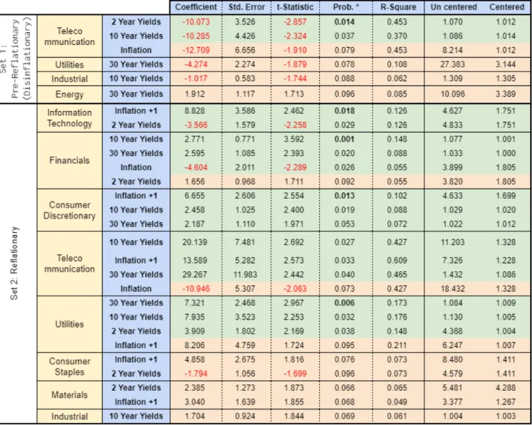
The model used 2, 10 & 30 -year interest rates and unadjusted CPI data to measure inflation. To supplement the analysis and see if there is a relation to expected inflation or inflation that comes before the increase could be reflected in the CPI data, regressions were also run with inflation applied from future period (inflation +1). Only results with a 10 % significance level or lower were summarized below, where the light orange color indicates results fitting in a 10 % significance level and the light green color indicates fitting to a 5%. Full regression tables and results are available in the appendix. For summarized results of regression outputs significance levels, see table A15

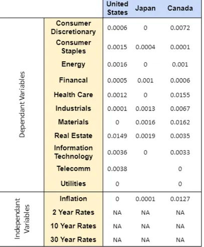
5.2.2 Data tests

The time-series data was tested for a unit root using nothing, random walk, and random walk with a drift. When correcting the data for a unit root, the first difference was taken, using any significance above 0.05 as an indicator for the data having a unit root. This was done in order to prevent running a spurious regression and getting misrepresentative p-values of the coefficients. First difference was taken for Telecommunications, 2 year and 10 year interest rates under time range set 1, while for time range set 2 it was done for Telecommunications, 10 year and 30 year interest rates.

Each regression was tested for serial correlation and heteroskedasticity using a Breusch Godfrey LM test and a Breusch Pagan Godfrey heteroskedasticity test. In some cases, the regressions had to be corrected by implementing either Hac Newey West standard errors to adjust for the serial correlation or Huber White standard errors to adjust for the heteroskedasticity issues. The corrected output is already shown within the results and the test summary can be seen in the Appendix’s Table A14. Since the independent variables might be correlated, the regression was also tested independently for multicollinearity using VIF. Most independent variables indicated no signs of multicollinearity, being within a range of 1 to 3 for the VIFs uncentered and centered tests. There were a few sectors such as the Telecommunications that had relatively consistent high VIF uncentered scores as well as some regressions that used future inflation had scores between 4-9. In most cases, such as the Telecommunication sector, multicollinearity issues can be caused by relatively low amounts of observations. However, Hair (Hair et al., 1995) states that the max acceptable VIF is 10, which depends a lot on the research topic, hence concluding that there were no significant issues with multicollinearity in the regression results.

(23)

5.2.3 Regression Results

In time range 1, when the economy is in a disinflationary period right before a reflationary pivot, analysis shows that most of the sectors did not have a statistical relation with inflation or interest rates. The only market sector that had significant results was the telecommunications sector with a strong significance, particularly with the 2 and 10-year interest rates, With a p-value of 0.014 & 0.037 for the interest rates, and a negative coefficient of around -10 for both. Indicating that, during the times prior to a reflationary period, these sectors benefited from the dropping inflation rates. Also, R-square was very high for both being 0.453 & 0.37, thus indicating that the variables could have explained 37 % of the changes in yearly sector performance. The results showed that in a decreasing inflation environment, if interest rates spiked, the Telecommunication sector would be impacted negative 10% for every 1% of interest rate increase.

Utilities, Industrials and Energy showed some sensitivity towards interest rates that would fit in a 10% significance level with p-value equal to or less than 10%. However, Utilities and Energy tested for high VIF uncentered, indicating there could be some multicollinearity issues, thus leaving the Industrials sector that would similarly to the Telecommunications sector, perform negatively with rise in the interest rates, however, with a much lesser negative impact of -1% of performance to every 1% increase in rates.

More interesting results came from the reflationary data set that followed a period of disinflation, with several different sectors showing high significance fitting in 5% and even 1% significance levels. The Information technology sector showed positive performance towards rising expected inflation with a significant p-value of 0.018, however, it would get negatively impacted when 2 year yields would start to increase with a significance of 3%.

Opposite to the Information Technology sector, the Financial sector would get negatively impacted by rising inflation with a significance level of 3% and positively impacted by a rise in interest rates, though impacted more by longer-term 10 and 30 year rates. The results were the only ones in the study fitting into 0.01% significance level.

Consumer Discretionary and Telecommunication sectors had a significant positive impact from both rising 10 and 30 year interest rates and higher future inflation, with Telecommunications showing more than double the positive performance impact from increasing interest rates than Consumer Discretionary sector. R-square was also high for the Telecommunications sector, signaling that over 40% of variance was explained by the model, however, there could have been some multicollinearity issues as VIF uncentered was fairly high on 10 Year yields and Inflation +1 that could have been caused due to relatively smaller sample size than other sectors caused by less countries tracking this sector.

Finally, the Utilities sector showed positive relation to all term interest rates with a significance varying from 4% to 1%, however, not much relation was found towards inflation that would fit into the 5% significance level.

(24)

Table 6 : Significant Regression Results for time range 1 & 2 combined, sorted by significance Full details of regression can be found in table A8-A13 in the appendix.

(25)

5.3 Analysis Summary

Looking at the overall analysis from the correlation matrix, it can be seen that, in general, interest rates are positively correlated with inflation, as expected. While there were several statistically significant results, several sectors stood out from the group.

Energy is one of them, showing high sensitivity to inflation that resulted from the United States non -historic time-specific data set. The analysis showcased that for every 1% of inflation increase, the Energy sector’s performance would be positively impacted by 7.5%. Results fit into 99% significance with 20% of the performance explained by inflation. Regression results were also in line with correlation analysis, which indicated that Energy is 43% correlated with a very significant p-value of 0.017. Interestingly, in Canada, the regression results indicated an opposite result for the Energy sector, with a negative impact for every point of inflation increase. However, the significance is much lower with a p-value of 0.06 and the correlation analysis did not show any significance between inflation and Energy, hence results from Canada can most likely be ruled out. Surprisingly, no significant findings came out for the Energy sector from inflection data sets, though lack of findings could have resulted from lack of data points, as the most extensive historic inflationary inflection points were in the 1920s and 1970s, while data sets for sectors mainly were from the 1980s and later. The Telecommunications sector had interesting findings showing that, in a disinflationary environment, prior to a reflationary one, the sector’s performance is negatively impacted by an increase of interest rates, however, in a reflationary period, it becomes positively impacted. The Telecommunications sector is very capital investment dependent. This could indicate that, in a decreasing inflation and interest rate environment, the sector performs well by being able to expand infrastructure relatively cheaper, while afterward benefiting from appreciating capital in a reflationary environment.

Another finding was that the Financial sector showed a highly statistically significant (p-value <0.001) positive performance towards a 10-year interest rate increase in a reflationary period. This could be caused by higher profit margins from existing loans that do not have a fixed rate, especially as, in a disinflationary period, the number of loans due to low interest rates tends to increase. The study also showed that the Financials sector, in a reflationary environment, would be impacted negatively by a rise in inflation, until the interest rates catch up and rise as well.

Information Technology showed unconventional results. As seen on the correlation analysis, usually, interest rates are positively correlated with inflation, however, while the sector showed statistically significant positive impact by future inflation, at the same time an increase in short-term interest rates would negatively impact the sector - indicating that, in a reflationary period, inflation actually benefits the Information Technology sector, as long as interest rates are not going up. This could be related to the Information Technology sector being highly growth oriented with future valuations very dependent on how much growth can be achieved, however, with rising interest rates, access to capital as well as debt maintenance will be more expensive, putting a direct impact on how much growth can be achieved.

Consumer Discretionary showed very significant, fitting almost into 99%, confidence level, 7% positive performance to every 1% of increasing inflation and to some extent increasing interest rates. This could indicate that as inflation increases and theoretical value money drops, it encourages consumer spending in certain industries of the sector, such as Consumer Durables or Automobiles.

(26)

Interestingly, except for the Financials sector, the statistically significant sectors from the regression during a reflationary period (with p-value < 0.10) were only sensitive to a rise of interest rates and future inflation, rather than the unadjusted CPI inflation. This could indicate that CPI inflation is lagging to reflect the impact of inflation in the sectors and that the bigger impact is caused by change in interest rates and real world inflation rather than change of reported CPI data.

5.4 Comparing Findings to Theory

Reflecting back on the results in conjunction with the theory, the outcome is a mixed bag of findings of which some aligned well with the theory, while others were interesting surprises.

Just as Schroders Asset Management Company’s research on the 1970s concluded that the Energy sector has thrived in a high inflation environment - this study could verify, in the United States, a very statistically significant historical sensitivity and correlation to inflation that fit in the 99% confidence range. It was interesting to see that Energy was the only sector that showed significant results when looking at overall historical sector performance. Even though, there was no significant relation found when looking at various inflection points across different countries, however, that could be because of the sample size and range discussed under “6.2 Data observations”.

A surprising find was that, during a disinflationary period prior to reflation, there were very few sectors that showed significant results towards inflation or interest rates, and the only few that did were only sensitive to change in interest rates rather than inflation. A completely different picture was from a reflationary period data set, where there were many more sectors with significant results towards interest rates and upcoming future inflation. It could indicate that sectors might be more sensitive to the shock of inflection rather than to actual change in the drivers. This could be what Wolfgang was referring to when he mentioned that during inflationary inflection points, entities, businesses, and individuals are often caught off guard and unprepared for the change in economic drivers.

Study revealed that some sectors, such as Consumer Discretionary and Information Technologies, are more sensitive to changes in inflation while others like Financials, Utilities and Telecommunications are more responsive to changes in interest rates. This is in line with theory as sectors that are positively impacted from inflation like Consumer Discretionary could be more impacted from increasing the demand for consumption, while sectors with high leverage and capex expenditures like Financials or Utilities are more sensitive to change in interest rates rather than inflation.

Finally, the lack of results towards real asset sectors fell short of expectations. According to Wolfgang’s research, there should have been significant outperformance of sectors such as Materials or Real Estate, however, no such relation with high enough significance was observed in the current model.

(27)

6. Final thoughts

6.1 Conclusion

As the stage is being set and the likelihood for another inflationary period that could echo the 1970s keeps increasing, the value of research on the impact of inflation on the markets should only be increasing for investors. While this study confirmed that inflation does indeed cause prevailing trends in capital rotation impacting sector performance and uncovered some interesting dynamics in some sector’s behavior as a response to change in inflation and interest rates, there were topics related to commodities covered by theory and previous research that could not be validated. Further research on this topic is not only important for maximizing preparedness and acquiring tools to fully take advantage of potential reflationary opportunities, but also to spread awareness of this under-researched topic. Even though some countries such as Venezuela have experienced high inflation more recently, the United States is one of the financial market leaders as well as other major economies that have not had a long-term reflationary period for more than 20 to 30 years. Due to that, it may be easy to fall towards optimism bias and believe that such a negative event will not happen, however, various extremes in economies are pointing towards the other direction. Thus, it will be interesting to follow the development of the topic as well as to observe how the current economic extremes unfold in the upcoming decade.

6.2 Data Observations

One of the main factors that could have impacted the study results was a relative lack of historic sector performance data. For most countries, sector performance data does not go back very far, usually stopping in the 1980s or even closer to the 2000s. As the major historic market inflationary inflection pivots happened in the 1930s and 1970s, the lack of sector behavioral data forces the study to focus more on what Ray Dalio called short-term cycles rather than long-term cycles. While there are still effects observed, much of the sector behavior could have been muted, not significant enough or impacted by temporary trends or policy interventions during these short-term cycles. This could explain why, despite the Inflationary Cycle theory, results were relatively insignificant towards the commodity sectors.

The study used core CPI data to measure inflation, which generally represents inflation quite well but not without flaws. It can take time until an increase in inflation gets reflected by CPI, which would cause inaccuracies in the timeline between sector performance and inflation. Also, inflation expectations may impact various sectors as much as inflation itself, however, as there is not enough inflation expectation data, the study used CPI inflation, which was forwarded by one period, to try and mimic this. This would lead to the assumption that inflation expectations would always be correct and not reflect sector impact due to incorrect expectations. In addition, splitting the sectors between commodity based and non commodity based, and using Producer Price Index (PPI) for commodity based sectors could have yielded more significant results towards the commodity sectors. Graph A6 was included in the appendix for reference that compares CPI and PPI for the United States.

Finally, yearly data points were used instead of monthly. The lesser amount of points could cause a decrease in the resolution of the study, potentially affecting the results.

(28)

6.3 Future Research

Based on world economic driver indications such as historic low-interest rates, historically longest disinflationary period as well as certain sector extremes, world economies may be at a long-term pivotal point towards an extended reflationary period. In conjunction with the demographic reversal, increasing inflation may become the norm in the foreseeable future. Due to the lack of information on this topic and its relevance in today's world, it would be interesting to see more research expanding on this subject.

One thing that could enrich the study is to look at lower than sector levels such as industry or industry groups. This could bring additional insight into industries performing differently than the whole sector. For example, this study showed a very significant dependency for the Financials sector on interest rates, however, if looked deeper, potentially the Insurance industry might not have performed as well as the Banking industry, or vice versa. Another example could be the commodity sector, steel might not perform equally to copper, or oil and gas might show different results than coal.

Another useful study could be to use a different model in analysis, which would be more sensitive to time progression. This would allow tracking sectors across the reflationary time period, potentially revealing trends between the sectors that are impacted sooner in the cycle or later. Also, the rate of inflation change could affect a sector differently across the timeline. A big inflationary spike that does not last too long as it is followed by lower inflation might have a different impact on sectors compared to sustained medium inflation across the same time period.

While the amount of control variables was limited in this study, in an analysis of specific countries and sectors (or industries under a specific sector) introducing more control variables could be beneficial in isolating the impact of inflation.

Increase in data sample and the amount of inflection points could increase the significance of specific sectors that fit between 90% and 95% confidence range. One of ways to increase data samples could be by using consolidated data from “EU KLEMS Growth and Productivity Accounts: Statistical Module” data set that has industry and industry group level data for all European countries and the United States.

While according to Ray Dalio analysis, all countries experience the same inflation and debt cycles, the strength of various cycle phases and impact on sectors could be different between individual countries. Thus when analysing specific market conditions for reasons such as investing, an aggregate of various country sector performance that this study used might not be enough. A better and more investable result could be achieved by analysing specific market and country conditions.

Finally, while this paper looked at the overall performance of various market sectors, it could bear fruit from looking at relative outperformance between sectors to one another. This way various risk profiles could be determined in a certain inflationary environment, which could be helpful in building portfolios with a specific risk profile.

(29)

7. Reference List

Amadeo, K. (2021). How the Fed Controls Inflation. The Balance. Retrieved 10 April 2021, from

https://www.thebalance.com/what-is-being-done-to-control-inflation-3306095.

Amadeo, K. (2021). How Bad Is Inflation? Past, Present, Future. The Balance. Retrieved 1 May 2021, fromhttps://www.thebalance.com/u-s-inflation-rate-history-by-year-and-forecast-3306093.

Amadeo, K. (2021). US National Debt by Year Compared to GDP and Major Events. The Balance. Retrieved 4 May 2021, from

https://www.thebalance.com/national-debt-by-year-compared-to-gdp-and-major-events-3306287.

Bethlehem, G. 1972, ‘An investigation of the return on ordinary share [sic] quoted on The Johannesburg Stock Exchange with reference to hedging against inflation’, The South African Journal of Economics, vol. 40, no. 3, pp. 254-267.

BofA Global Investment Strategy (2021), Big Tech the Beneficiary of Central Bank Largesse. Retrieved fromBusiness SourceBloomberg database.

BofA Global Equity Strategy (2021). Commodities Rolling Returns. Retrieved from Global Financial Data, Bloomberg.

Schroders Asset Management Company (2014), Investment Perspectives: What are the inflation beating asset classes?

https://www.schroders.com/en/sysglobalassets/staticfiles/schroders/sites/americas/canada/documents/i nvestment-perspective-what-are-the-inflation-beating-asset-classes.pdf

Buffett Indicator Shows Stock Market is Overvalued. Currentmarketvaluation.com. (2021). Retrieved 4 May 2021, fromhttps://currentmarketvaluation.com/models/buffett-indicator.php.

Cage, M. (2021). $ 9 Trillion Story: 22% of the Circulating USD Printed in 2020 - Somag News. Retrieved 14 April 2021, from

https://www.somagnews.com/9-trillion-story-22-of-us-dollars-printed-in-2020/

Canada Inflation Rate 1960-2021. Macrotrends.net. (2021). Retrieved 2 March 2021, from

https://www.macrotrends.net/countries/CAN/canada/inflation-rate-cpi.

Canada Sector Composition S&P/TSX Composite Index (GSPTSE) - Investing.com. Investing.com. (2021). Retrieved 2 March 2021, fromhttps://www.investing.com/indices/s-p-tsx-composite.

Canada 2-Year Bond Yield - Investing.com. Investing.com. (2021). Retrieved 2 March 2021, from

https://www.investing.com/rates-bonds/canada-2-year-bond-yield.

Canada 10-Year Bond Yield - Investing.com. Investing.com. (2021). Retrieved 2 March 2021, from

https://www.investing.com/rates-bonds/canada-10-year-bond-yield.

(30)

China Inflation Rate 1987-2021. Macrotrends.net. (2021). Retrieved 2 March 2021, from

https://www.macrotrends.net/countries/CHN/china/inflation-rate-cpi.

China Sector Composition. Shanghai Composite Index (SSEC) - Investing.com. Investing.com. (2021). Retrieved 2 March 2021, fromhttps://www.investing.com/indices/shanghai-composite.

Dalio, R. (2017). How the Economic Machine Works - Leveragings and Deleveragings (1st ed., pp. 2-10). Bridgewater.

https://economicprinciples.org/downloads/ray_dalio__how_the_economic_machine_works__leveragi ngs_and_deleveragings.pdf/.

Federal Reserve Bank of St Louis. (2021). Energy equities maintained strong returns through the high inflation 1970's. Datastream.

France Inflation Rate 1960-2021. Macrotrends.net. (2021). Retrieved 2 March 2021, from

https://www.macrotrends.net/countries/FRA/france/inflation-rate-cpi.

France Sector Composition. CAC 40 Index (FCHI) - Investing.com. Investing.com. (2021). Retrieved 2 March 2021, fromhttps://www.investing.com/indices/france-40.

France 2-Year Bond Yield - Investing.com. Investing.com. (2021). Retrieved 2 March 2021, from

https://www.investing.com/rates-bonds/france-2-year-bond-yield.

FTSE/JSE Top 40 Index (JTOPI) - Investing.com. Investing.com. (2021). Retrieved 2 March 2021, fromhttps://www.investing.com/indices/ftse-jse-top-40.

Germany Inflation Rate 1960-2021. Macrotrends.net. (2021). Retrieved 2 March 2021, from

https://www.macrotrends.net/countries/DEU/germany/inflation-rate-cpi.

Germany Sector Composition DAX Index Today (GDAXI) - Investing.com. Investing.com. (2021). Retrieved 2 March 2021, fromhttps://www.investing.com/indices/germany-30.

Germany 2-Year Bond Yield - Investing.com. Investing.com. (2021). Retrieved 2 March 2021, from

https://www.investing.com/rates-bonds/germany-2-year-bond-yield.

GESKE, R., & ROLL, R. (1983). The Fiscal and Monetary Linkage between Stock Returns and Inflation. The Journal Of Finance, 38(1), 1-33.https://doi.org/10.1111/j.1540-6261.1983.tb03623.x

GICS - Global Industry Classification Standard. Msci.com. (2021). Retrieved 1 March 2021, from

(31)

Golubova, A. (2021). Rapid recovery in 2021: 'We'll be shocked at how strong economy comes back' but risks remain, say analysts. Kitco News. Retrieved 16 April 2021, from

https://www.kitco.com/news/2020-12-21/Rapid-recovery-in-2021-We-ll-be-shocked-at-how-strong-ec onomy-comes-back-but-risks-remain-say-analysts.html.

Goodhart, C., & Pradhan, M. (2020). The Great Demographic Reversal: Ageing Societies, Waning Inequality, and an Inflation Revival (1st ed., pp. 4-5, 11-13, 58-70). Palgrave Macmillan

G. S. BAKSHI – Z. CHEN (1996), “Inflation, Asset Prices, and the Term Structure of Interest Rates in Monetary Economies”. Review of Financial Studies, 9, pp. 241-275

Gujarati, D. N. (1988).Basic Econometric. New York: John Wiley.

Hair, J. F. Jr., Anderson, R. E., Tatham, R. L. & Black, W. C. (1995). Multivariate Data Analysis (3rd ed., pp. ). New York: Macmillan..

H. Hammes, W. (2016). The Return of High Inflation: Risks, Myths, and Opportunities (1st ed., pp. 27-43, 114-169, 245-251). Vangi Group LLC.

India Inflation Rate 1960-2021. Macrotrends.net. (2021). Retrieved 2 March 2021, from

https://www.macrotrends.net/countries/IND/india/inflation-rate-cpi.

India Sector Composition. Nifty 50 Index (NSEI) - Investing.com. Investing.com. (2021). Retrieved 2 March 2021, fromhttps://www.investing.com/indices/s-p-cnx-nifty.

IMF. (2016). Global Disinflation in an Era of Constrained Monetary Policy. World Economic Outlook, 121-125.

Japan Inflation Rate | 1958-2021 Data | 2022-2023 Forecast | Calendar | Historical. Tradingeconomics.com. (2021). Retrieved 1 May 2021, from

https://tradingeconomics.com/japan/inflation-cpi

Japan Nikkei 225 Index - 67 Year Historical Chart. Macrotrends.net. (2021). Retrieved 1 May 2021, fromhttps://www.macrotrends.net/2593/nikkei-225-index-historical-chart-data.

Japan sector composition. TOPIX Index (TOPX) - Investing.com. Investing.com. (2021). Retrieved 1 March 2021, fromhttps://www.investing.com/indices/topix.

Japan 2-Year Bond Yield - Investing.com. Investing.com. (2021). Retrieved 2 March 2021, from

https://www.investing.com/rates-bonds/japan-2-year-bond-yield.

https://www.investing.com/rates-bonds/japan-10-year-bond-yield.

The Impact of Inflation on Capital Rotation in Inflationary Inflection Points : An Investigation on How Inflation Affects Capital Rotation Between Major Market Sectors as Economies Shift from Disinflation to Reflation