AN ANALYSIS OF LANDSLIDE VOLUME, STRUCTURES, AND KINEMATICS FROM SATELLITE IMAGERY OF THE 2016 LAMPLUGH ROCK AVALANCHE,
GLACIER BAY NATIONAL PARK AND PRESERVE, ALASKA
by
A thesis submitted to the Faculty and the Board of Trustees of the Colorado School of Mines in partial fulfillment of the requirements for the degree of Master of Science (Geological Engineering). Golden, Colorado Date: __________________________________ Signed: ________________________________________ Erin K. Bessette-Kirton Signed: ________________________________________ Dr. Wendy Zhou Thesis Advisor Golden, Colorado Date: ________________________________________ Signed: ________________________________________ Dr. Stephen Enders Department Head Department of Geology and Geological Engineering
ABSTRACT
During the past five years occurrences of large rock avalanches over glaciated terrain in Glacier Bay National Park and Preserve (GBNP), Alaska have drawn attention to the complex, highly variable, yet poorly understood dynamics of these events. The objective of this research is to study the emplacement processes of the Lamplugh rock avalanche through an analysis of the volume and distribution of material in conjunction with structures and surficial features within the deposit. This research demonstrates the ability to use high-resolution remotely sensed data to study rock avalanches in glaciated terrain and provides an improved framework with which to estimate many of the uncertainties affecting volume measurements in glacial environments. The Lamplugh rock avalanche occurred on June 28, 2016 and is the largest rock avalanche on record in GBNP. WorldView satellite stereo imagery was used to derive pre- and post-event, high-resolution (2m) Digital Elevation Models (DEMs). Differenced DEMs were used to calculate both source and deposit volumes and examine variations in deposit thickness. DEMs were also used in conjunction with high-resolution (~0.5m) optical imagery to map landslide structures and surficial features. The characterization of landslide structures and the evaluation of volume and thickness were used to make interpretations about emplacement processes. Unmeasured ice changes between the acquisition of pre- and post-event imagery and the rock avalanche
occurrence were found to underestimate the total volume of deposited material by 91%. A large amount of surficial material downslope of the source area, much of which was likely snow and ice, was scoured and entrained during emplacement. The rock avalanche deposit is also
characterized by lateral and distal rims that are significantly thicker than the interior of the deposit. The examination of overall deposit geometry in addition to the identification of structures and surficial features within the deposit indicates that emplacement occurred as multiple surges of failed rock avalanche material. An improved understanding of rock avalanche processes is critical to future hazard assessments of rock avalanches travelling on ice within GBNP and in other glaciated regions.
TABLE OF CONTENTS
ABSTRACT ... iii
LIST OF FIGURES ... vii
LIST OF TABLES ... x
ACKNOWLEDGMENTS ... xii
CHAPTER 1 INTRODUCTION ... 1
CHAPTER 2 BACKGROUND ... 5
2.1 Prior Work ... 5
2.1.1 Inventory of Rock Avalanches in Glacier Bay National Park and Preserve... 5
2.1.2 Morphologies and Structures of Rock-Avalanche Deposits ... 6
2.2 Study Area and the Lamplugh Rock Avalanche ... 10
CHAPTER 3 PURPOSE ... 15
CHAPTER 4 METHODS ... 16
4.1 WorldView Imagery ... 16
4.1.1 Acquired Imagery ... 17
4.2 Elevation Datasets ... 19
4.3 Ames Stereo Pipeline Workflow ... 19
4.3.1 Pre-processing and Pre-alignment ... 20
4.3.2 Stereo Correlation ... 21
4.3.3 Raster Conversion ... 23
4.4 DEM Generation ... 23
4.5 DEM Accuracy Analysis ... 24
4.6 DEM Differencing ... 26
4.7.1 Scenario 1: Areas of Net Positive Elevation ... 28
4.7.2 Scenario 1: Areas of Net Negative Elevation ... 30
4.7.3 Scenario 2: Areas of Net Positive Elevation ... 31
4.7.4 Scenario 2: Areas of Net Negative Volume ... 32
4.7.5 Scenario 3: Areas of Net Positive Volume ... 33
4.7.6 Scenario 3: Areas of Net Negative Volume ... 35
4.8 Volume, Thickness, and Center of Mass ... 36
4.8.1 Volume ... 37 4.8.2 Average Thickness ... 37 4.8.3 Center of Mass ... 37 4.9 Structural Mapping ... 38 CHAPTER 5 RESULTS ... 40 5.1 DEM Generation ... 40
5.2 DEM Accuracy Analysis ... 40
5.3 Differenced DEMs... 42
5.4 Elevation Adjustments... 45
5.5 Volume, Thickness, and Center of Mass ... 48
5.5.1 Volume and Average Thickness ... 48
5.5.2 Center of Mass ... 54 5.6 Structural Mapping ... 55 5.6.1 Strike-slip faults ... 55 5.6.2 Thrust faults ... 57 5.6.3 Fault scarps ... 57 5.6.4 Transverse ridges ... 59
5.6.5 Fensters ... 59
5.6.6 Run-up ... 62
CHAPTER 6 DISCUSSION ... 63
6.1 Independent Checks on Volume Analysis Methodology ... 63
6.1.1 Seasonal Snow and Ice Change ... 63
6.1.2 Ice Insulation and Differential Melting... 65
6.1.3 Volume Calculation ... 67
6.1.4 Improvements on Volume Estimates ... 69
6.2 Deposit Geometry Comparisons... 71
6.3 Emplacement Hypotheses ... 76 CHAPTER 7 CONCLUSION... 82 REFERENCES ... 84 APPENDIX A ... 91 APPENDIX B ... 93 APPENDIX C ... 94 APPENDIX D ... 95
LIST OF FIGURES
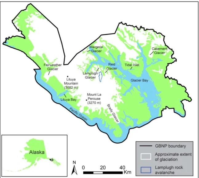
Figure 2-1. Map of Glacier Bay National Park and Preserve showing the location of the Lamplugh rock avalanche (Alaska Department of Natural Resources, Information Resource Management, 1998a, 1998b; National Park Service, 2014) ...11 Figure 2-2. Profile of pre-event topography along the travel path of the Lamplugh rock
avalanche. ... 13 Figure 4-1. Digital Globe Inc. image collected on 8/27/2016 showing the location of the six
control areas used to assess the relative accuracy of DEMs produced in ASP. ... 25 Figure 4-2. Diagram showing the effect of unmeasured changes in surface elevation between
the acquisition of pre-event imagery collected on 6/15/2016 and post-event imagery collected on 7/16/2016 and the occurrence of the Lamplugh rock
avalanche on 6/28/2016 in deposit areas with net positive volumes. The elevation of the glacier surface at time ti (light blue line) is subtracted from the surface elevation measured at time tf (red line) during DEM differencing. The thickness of the deposit measured by DEM differencing (h2) is not equivalent to the actual thickness of the deposit (thtrue). True deposit thickness can be measured by summing the difference in elevation on the adjacent glacier surface between ti and tf (h1) with h2. ... 29 Figure 4-3. Diagram showing the effect of unmeasured changes in surface elevation between
the acquisition of pre-event imagery collected on 6/15/2016 and post-event imagery collected on 7/16/2016 and the occurrence of the Lamplugh rock
avalanche on 6/28/2016 in deposit areas with net negative volumes. The elevation of the glacier surface at time ti (light blue line) is subtracted from the surface elevation measured at time tf (red line) during DEM differencing. Neither the height of scoured and entrained material (hentrained) nor the height of material deposited in the scoured area are represented by the change in elevation measured between ti and tf in areas of the deposit (h2n). Elevation change on the adjacent glacier surface between ti and tf is represented by the height of h1n. The actual thickness of entrained material can be measured by subtracting h1n from the sum of h2n and hfill. ... 31 Figure 4-4. Diagram showing the added effect of differential ice melt on ice changes that are
not measured during DEM differencing in net positive deposit areas. The change in height of the deposit, either due to melting of underlying ice or melting and densification within the deposit is assumed to be zero. The actual thickness of the deposit (thtrue) is measured by subtracting the elevation change on the adjacent surface between te and tf (h3) from the sum of h1 and h2. When observed from an adjacent location in space the presence of differential ice melt causes the
observed deposit thickness (thapparent) to be greater than thtrue. ... 33 Figure 4-5. Diagram showing the added effect of differential ice melt on ice changes that are
in height of the deposit, either due to melting of underlying ice or melting and densification within the deposit is assumed to be zero. The actual thickness of entrained material (hentrained) is measured by subtracting h1n from the sum of h2n and hfill and the change in elevation on the adjacent surface between te and tf (h3n). ... 34 Figure 4-6. Diagram showing the added effect of post-depositional elevation changes within
the rock avalanche deposit on ice changes that are not measured during DEM differencing in net positive deposit areas. The actual thickness of the deposit (thtrue) is measured by subtracting (h3) from the sum of h1, h2, and the change in elevation within the deposit between te and tf (h4). ... 35 Figure 4-7. Diagram showing the added effect of post-depositional elevation changes within
the rock avalanche deposit on ice changes that are not measured during DEM differencing in net negative deposit areas. The actual thickness of entrained material (hentrained) is measured by subtracting the sum of h1n and the change in elevation within the deposit between te and tf (h4n) from the sum of h2n, hfill, and h3n. ... 36 Figure 5-1. Elevation difference in Control Areas 4-6 between 6/15/2016 and 7/16/2016. ... 42 Figure 5-2. Elevation difference between pre- (6/15/2016) and post-event (7/16/2016) DEMs
over the Lamplugh rock avalanche deposit. Dashed line indicates extent of source area, which is obscured by clouds in the image acquired on 7/16/2016. ... 43 Figure 5-3. Elevation difference between pre- (6/15/2016 and SDMI 5-meter) and post-event
(9/27/2016) DEMs in the source area of the Lamplugh rock avalanche. ... 45 Figure 5-4. Differenced DEMs between a) 7/16/2016-8/27/2016 and b) 8/27/2016-9/28/2016
showing post-event changes within the Lamplugh rock avalanche deposit and on the adjacent glacial surface. ... 46 Figure 5-5. Adjusted elevation difference between pre- and post-event DEMs over the
Lamplugh rock avalanche. Data in the source area are from a 5-meter resolution SDMI DEM (pre-event) and an ASP-generated DEM from 9/27/2016 (post-event). Data within the remainder of the deposit are derived from ASP DEMs from 6/15/2016 (pre-event) and 7/16/2016 (post-event). ... 50 Figure 5-6. Zones of the Lamplugh rock avalanche delineated based on areas of accumulation
and depletion identified in the adjusted differenced DEM between 6/15/2016 and 7/16/2016 (Figure 5-5). ... 52 Figure 5-7. Generalized representations of structures and surficial features (1:48,000 scale)
mapped on a Digital Globe, Inc. image (7/16/2016) of the Lamplugh rock
Figure 5-8. Strike-slip movement along the distal margin of the Lamplugh rock avalanche deposit exemplified in a) Digital Globe, Inc. imagery from 7/16/2016 and b)
adjusted differenced DEM between 6/15/2016 and 7/16/2016 (Figure 5-5). ... 58
Figure 5-9. Digital Globe, Inc. image taken on 7/16/2016 showing transverse ridges in the toe of the Lamplugh rock avalanche. ... 60
Figure 5-10. Example of fensters identified in a) Digital Globe, Inc. imagery from 7/16/2016 and b) adjusted differenced DEM between 6/15/2016 and 7/16/2016 (Figure 5-5). Profile a-a' was derived from the post-event (7/16/2016) DEM. ... 61
Figure 5-11. Digital Globe, Inc. imagery from 7/16/2016 showing locations of run-up along the west lateral margin of the Lamplugh rock avalanche. ... 62
Figure 6-1. Differenced cross-sections taken along a transverse profile through the deposit toe between 6/15/2016-7/16/2016 and 6/15/2016-8/27/2016. An increase in observed thickness (Δ = 2.7 meters) with an increase in time between observations demonstrates differential melting between deposit-covered areas and the adjacent surface. ... 66
Figure 6-2. Normalized differenced cross-sections through the toes of the Lamplugh and West Salt Creek rock avalanches show a difference in relief between the distal rim and more proximal areas of the deposit. ... 73
Figure 6-3. Plots of Lmax versus L for a) rock avalanches travelling over rock/soil and ice and b) confined and unconfined rock avalanches. ... 76
Figure A-1. Elevation difference in Control Areas 4-6 between 7/16/2016 and 8/27/2016...91
Figure A-2. Elevation difference in Control Areas 4-6 between 8/27/2016 and 9/28/2016...91
Figure A-3. Elevation difference in Control Areas 1-3 between SDMI 5m- and 9/27/2016...92
Figure A-4. Elevation difference in Control Areas 1-3 between 6/15/2016- and 9/27/2016...92
Figure B-1. Digital Globe, Inc. image of the Lamplugh rock avalanche on 7/16/2016 that was used for mapping of structures and surficial features……….…93
Figure C-1. Pre- and post-event elevation profiles along A-A' showing the location of Zones A-F. Pre-event elevation data is derived from a 5-meter resolution SDMI DEM (source area only) and the ASP-generated DEM from 6/15/2016. Post-event elevation data is derived from DEMs from 9/27/16 (source area only) and 7/16/2016...94
LIST OF TABLES
Table 2-1. Characteristics of previously documented rock avalanches travelling on ice, with areas larger than 1 km2, in Glacier Bay National Park and Preserve. ... 13 Table 4-1. Panchromatic and multispectral sensor resolution and geolocation accuracy of
WorldView-1, 2, and 3 satellites (DigitalGlobe, Inc. 2016b, 2016c, 2016d). ... 16 Table 4-2. Horizontal (CE90) and vertical (LE90) geolocation accuracy of WorldView-1, 2,
and 3 satellites (DigitalGlobe, 2016a, 2016d). ... 17 Table 4-3. Dates of pre- and post-event Digital Globe, Inc. imagery acquired for DEM
generation and mapping of the Lamplugh rock avalanche. ... 18 Table 4-4. Average slope of each control area used to assess the accuracy of differenced
DEMs over the Lamplugh rock avalanche. ... 24 Table 4-5. Dates and uses of differenced DEMs for analysis of the Lamplugh rock avalanche. . 27 Table 5-1. Mean triangulation error in the north-south (Band 1), east-west (Band 2), and
vertical (Band 3) directions for each DEM produced in ASP. ... 40 Table 5-2. Results of the chi-square goodness-of-fit test, mean, IQR, standard deviation, and
relative vertical accuracy of elevation difference in control areas between DEM pairs used for differencing analyses. ... 41 Table 5-3. Elevation changes on the Lamplugh rock avalanche deposit and adjacent surfaces
measured as average total change and average daily rate of change between specified dates in June (pre-event), July, August, and September, 2016. Changes in elevation are measured on A) the glacier surface adjacent to areas of the deposit with a net positive volume, B) areas of the deposit with a net positive volume, C) the surface adjacent to areas of the deposit with a net negative volume, and D) areas of the deposit with a net negative volume. ... 44 Table 5-4. Measured and estimated parameters used in Equations 4-5 and 4-6 to calculate
elevation adjustments for differences in elevation between 6/15/2016 and 7/16/2016 in the area of the Lamplugh rock avalanche deposit. Since h2 and h2n are measured from the changes in elevation in the deposit area between 6/15/2016 and 7/16/2016, these values are unique for each pixel of the differenced DEM (Figure 5-2) and are not reported here (i.e., N/A entries). ... 47 Table 5-5. Deposit volumes and average thicknesses for each zone of the Lamplugh rock
avalanche... 54 Table 5-6. Longitudinal locations of the center of mass for the entire Lamplugh rock
avalanche deposit and for only the east (unconfined) and west (confined) halves of the deposit. ... 54
Table 6-1. Estimated snow and ice changes compared to the average elevation change observed on the glacier surface between 6/15/2016-7/16/2016,
7/16/2016-8/27/2016, and 8/27/2016-9/28/2016. ... 64 Table 6-2. Values of apparent and adjusted deposit volume and average thickness for each
zone of the Lamplugh rock avalanche. Please refer to Figure 5-6 for zone
delineation. ... 68 Table 6-3. Center of mass locations for rock avalanches travelling over rock/soil and ice and
ACKNOWLEDGMENTS
The U.S. Geological Survey provided funding and the opportunity for this research. I would like to acknowledge my committee member, Jeffrey Coe, from the U.S. Geological
Survey for helping me develop the vision for this research and for providing guidance throughout the project. I would also like to express my appreciation for my advisor, Dr. Wendy Zhou, and my committee member, Dr. Paul Santi, who provided suggestions and insight throughout the project. I would like to acknowledge the Department of Geology and Geological Engineering for providing funding throughout my graduate study. Finally, I would like to thank my peers in the Department of Geology and Geological Engineering and my colleagues at the U.S. Geological Survey for comments and advice throughout my research.
CHAPTER 1 INTRODUCTION
Slope instabilities are common in mountainous terrain and increasing development in these areas necessitates hazard analyses. Mass wasting of mountainous terrain in polar regions can be particularly complex because of interactions with glacial ice (Korup & Dunning, 2015) and the presence of alpine permafrost (Evans & Delaney, 2014). Catastrophic slope failures are particularly common in areas of Alaska, British Columbia, the European Alps, the Russian Caucasus, and the New Zealand Alps. Types of mass wasting in alpine areas include glacier avalanches, rock falls, debris flows, landslides in rock and soil, rock slides, and rock avalanches (Evans & Clague, 1994; Geertsema et al., 2006; Geertsema & Cruden, 2008). This research will focus on rock avalanches sourced from periglacial rock slopes that travel over ice. This type of mass movement (also commonly referred to as rock-ice avalanches) is characterized as a large volume, highly mobile failure that involves rapid, flow-like movement of rock and ice (Deline et al., 2015; Evans & Delaney, 2015). Rock-ice avalanches have the potential to be extremely catastrophic, with estimates of volumes greater than 109 m3 and velocities in excess of 100 m/s (Pudasaini & Krautblatter, 2014). Significant hazards can arise when rock-ice avalanches occur in populated mountain areas or when deposits travel significant distances from the location of failure into developed areas. Secondary effects of rock avalanches, including tsunamis
(Wieczorek et al., 2007), breached landslide dams (Korup & Dunning, 2015), and rapidly induced glacial advances (Hewitt, 2009) can also cause significant hazards.
Several notable factors contribute to an inadequate understanding of rock avalanche processes in glaciated environments. The infrequent occurrence and typically remote locations of rock-ice avalanches make direct detection and observation difficult. Recognition is further hindered by glacial processes and snow cover, which limit the preservation of characteristically
thin deposits (Deline et al., 2015). Additionally, misclassification of rock-avalanche deposits as moraines has caused an under representation of documented historic events (Deline et al., 2015). Many well studied rock avalanches on glaciers have been trigged by earthquakes, including the 1964 Alaska Earthquake (McSaveney, 1978; Post, 1967) and the 2002 Denali Fault earthquake (Jibson et al., 2006). Recent documentation of rock-avalanche events unprecedented in frequency and magnitude has drawn attention to climate change as an additional driving factor (e.g.
Geertsema et al., 2006; Gruber & Haeberli, 2007; Huggel et al., 2012). Glacial debuttressing and permafrost degradation have been causally linked to failures, however these processes are poorly understood and the exact mechanisms of individual failures remain ambiguous. The potential effect of increasing temperatures on slope stability in mountainous regions is especially relevant in light of recent warming trends and future climate predictions. Projections for temperature increases by 2055 in mid- and high-latitude alpine environments range from 3-4°C and 4-7°C, respectively (Krautblatter et al., 2012). Changes of this magnitude could have significant effects on the processes involved in rock-ice avalanche failures.
Landslide-hazard assessments rely on an accurate understanding of movement dynamics. The relationships between volume, area, and travel distance are particularly critical to assess the hazard potential of long-runout events (Legros, 2002). The complex and highly variable behavior of rock avalanches on glaciers corroborates the difficulty of predicting these geometric
parameters. Both empirical correlations (Evans & Clague, 1999; Schneider et al., 2011a) and numerical models (Bottino et al., 2002) suggest that the travel distance of rock avalanches travelling over ice exceeds that of rock avalanches travelling over other substrates. Several mechanisms exist to explain these observations, including: 1) the surface friction of ice is lower than that of rock or soil and 2) melting of entrained snow and ice increases the fluidity of debris
(Evans & Clague, 1999). Although empirical correlations and modeling have been shown to support this hypothesis, contradictory cases have also been cited. It has been shown that some rock-ice avalanches of similar volume have differing amounts of mobility (Evans & Clague, 1999) and that the mobility of some rock-ice avalanches travelling over glaciers have mobility values closer to those that would be expected from travel over soil or rock (Schneider et al., 2011a). These findings suggest that other unknown factors may also play a role in controlling the travel distance of rock-ice avalanches. Research involving both empirical relationships and numerical models has identified volume, topography, flow rheology (ice and water content), and frictional characteristics of the surface as the most significant factors influencing the
emplacement of rock-ice avalanches (Pudasaini & Krautblatter, 2014; Rosio et al., 2012; Schneider et al., 2011).
Volume estimations for rock-ice avalanches are difficult to obtain and routinely lack both accuracy and precision (Korup & Dunning, 2015; Schneider et al., 2011a). Many available literature values are crude estimates, made either based on deposit area and reported average thickness or by assuming that the relationship between volume and area is comparable to that of other similarly sized events (Sosio et al., 2012). Acquisition of high-resolution pre- and post-event topography data has been used to calculate volumes of other types of mass movements (e.g. Coe et al., 1997; Tsutsui et al., 2007) and could greatly improve rock-ice avalanche volume estimates.
Topography is also an important factor controlling the travel distance and path of rock-ice avalanches. Because rock-rock-ice avalanche deposits are typically thin, topographic control is more significant than it is for rock avalanches travelling over rock or soil (Rosio et al., 2012). The effects of micro-topographic variations (1-10 m) may have a more significant role in
controlling the mobility of flows over generally low gradient, smooth glacial surfaces compared to steep surfaces with variations in topography and surface roughness (Rosio et al., 2012; Schneider et al., 2011a).
Flow rheology and frictional characteristics of the sliding surface are harder to quantify than volume and topography and are significantly more difficult to study remotely. However, morphological features within landslide deposits reflect physical flow processes, which are directly affected by rheology and surface characteristics. Identification of structural features in both rock-avalanches on glaciers (e.g. Delaney & Evans, 2014; Dufresne and Davies, 2009; McSavaney, 1978) and on rock and soil (e.g. Coe et al., 2016; Dufresne et al., 2016) have been used to interpret the dynamics of mass movements.
Alaska has a rich history of rock-ice avalanches and during the past five years the occurrence of several large events in GBNP has drawn attention to this area. Most recently, the Lamplugh rock-ice avalanche occurred on June 28, 2016 (Petley, 2016) and is the largest event on record in GBNP (Bessette-Kirton & Coe, 2016; Post, 1967). The recent occurrence and exceptional size of this event make it an excellent candidate for a case study of the factors influencing rock-ice avalanche emplacement as a means of informing hazard assessments both within GBNP and in other glaciated regions. Additionally, the availability of high-resolution pre- and post-event imagery of the Lamplugh rock avalanche provides a platform through which the feasibility of using remotely sensed data to measure the volume of rock avalanches in remote areas can be assessed.
CHAPTER 2 BACKGROUND
2.1 Prior Work
This section describes a previous study on rock avalanches in GBNP and a number of other prior works that studied the morphology and dynamics of rock avalanches travelling over both ice and rock and soil.
2.1.1 Inventory of Rock Avalanches in Glacier Bay National Park and Preserve
This thesis is part of a larger a study by Bessette-Kirton and Coe (2016) which examines changes in frequency, magnitude, and mobility of rock avalanche events in GBNP since 1984. Landsat imagery (30-meter resolution) was used to create an inventory of rock avalanches in a 5000 km2 area of GBNP. Landsat images were used to identify and map 24 rock avalanches that occurred between 1984 and 2016. For each mapped rock avalanche the following parameters were recorded: date, or range in possible dates of occurrence, the total area covered by the rock avalanche (including the source area, travel path, and deposit), the maximum travel distance measured along a curvilinear centerline (L), and the maximum change in elevation between the start and end points of the centerline (H) (Bessette-Kirton & Coe, 2016).
Coe et al. (2017) conducted further analysis of the GBNP rock avalanche inventory and found that three main clusters of rock avalanches occurred during the period of study, the last of which began in June 2012 and includes four of the five largest rock avalanches in the inventory. An evaluation of rock avalanche characteristics shows that during the 33-year period of record, the magnitude (area) and mobility (as measured by H/L) of recorded rock avalanches increased (Coe et al., 2017). A slight increase in the recurrence interval of rock avalanches was also
in mean annual maximum air temperature exceeded 0° C in 2010, shortly before the start of the third cluster of large rock avalanches, indicates that temperature-related permafrost degradation may be related to the increasing size and occurrence of failures (Coe et al., 2017).
The inventory by Bessette-Kirton and Coe (2016) includes preliminary mapping of the Lamplugh rock avalanche. The Lamplugh rock avalanche occurred on June 28, 2016 and was recorded as a M=2.9 seismic event in the Alaska Earthquake Center catalog (Petley, 2016). In comparison to the other 23 events identified in the inventory of GBNP, The Lamplugh rock avalanche has the largest area (>2.5 times greater than the next largest) and is tied for the highest mobility (with a Height/Length=0.15). The geometric parameters obtained from 30-meter
resolution Landsat imagery could be refined with higher-resolution imagery.
2.1.2 Morphologies and Structures of Rock-Avalanche Deposits
Identification and analysis of depositional morphology, including overall geometries and the presence of relatively small structures, can provide insight into the sequence and
characteristics of rock avalanche emplacement. This type of investigation is particularly important to rock avalanche studies since failures are rarely witnessed. Observations of morphologic and structural features in rock avalanche deposits have been recognized as
important indicators of movement since the first published account of a rock avalanche, in which Heim described the 1881 Elm rock avalanche in Switzerland (as cited in Hsü, 1978). However, with a few exceptions, the majority of studies on deposit structures and surficial features rely on qualitative observations and localized measurements to draw conclusions about the overall mechanisms of emplacement. Additionally, the absence of sufficiently detailed pre- and post-event topography data for the majority of rock avalanche studies does not allow for a detailed
understanding of observations presented in the literature. The combination of field observations and detailed topographic data has the potential to provide valuable insight into rock avalanche emplacement processes.
Conceptual models have been used to describe rock avalanche deposit geometry as a basis for comparison with field data and observations. The deposit geometry of a simple or classic rock avalanche was described by Hewitt et al. (2008) as “an extensive thin sheet, rarely more than 2 to 10 m thick and lobate in plan… [which] varies little in thickness and has minor surface relief, commonly with a slight ridge at the distal rim.” This geometry has been
demonstrated experimentally (Friedmann et al., 2006) and in numerical models (Legros, 2002), but is rarely seen in nature because of topographic confinement (Hewitt et al., 2008) and interaction with or entrainment of substrate material (Dufresne, 2016; Hungr & Evans 2004). Additional thickness distribution models that have been corroborated by field observations vary based on the degree of confinement (Legros, 2002) and the type or progression of movement (Strom, 2006). The main types of thickness distributions identified in these models are: 1) a linear decrease in thickness with distance (Legros, 2002), 2) minimal variation in thickness with distance (Legros, 2002), and 3) a thin deposit at the proximal end with an increasing
accumulation of material towards the distal end (Strom, 2006). The thickness distribution models presented in the literature do not address rock avalanches travelling over ice. Limited field observations indicate that the average thickness of rock avalanches emplaced on glaciers is an order of magnitude less than that of rock avalanches travelling over rock and soil, (e.g. Jibson et al., 2006; McSaveney, 1978) with typical average thicknesses ranging from 0.5 to 5 meters (Deline et al., 2015).
Observations of deposit structures and surficial features have been used to make
interpretations about the mechanisms of rock avalanche emplacement in both prehistoric events (Dufresne et al., 2016; Eppler et al., 1987; Evans et al., 1994; Mudge, 1965) and modern rock avalanches travelling both over rock or soil (Hadley, 1978; Johnson, 1978; Marangunic & Bull, 1966; McSaveney, 1978; Shreve, 1966; Shreve, 1968) and ice (Cox and Allen, 2009; Delaney and Evans, 2014; Fahnestock, 1978; Jibson et al., 2006; Jiskoot, 2011; Lipovsky et al., 2008; McSaveney, 2002; Shugar and Clague, 2011). With the exception of a handful of studies (e.g. Tschirgant, Austria (Dufresne et al., 2016); Sherman Glacier, Alaska (Marangunic & Bull, 1966; McSaveney, 1978; Shreve, 1966); and West Salt Creek, Colorado (Coe et al., 2016)), detailed mapping of morphological and structural features in rock avalanche deposits has not been widely reported.
The most commonly recognized structures in rock avalanche deposits are sets of transverse and longitudinal ridges and furrows. Descriptions of transverse ridges (Jibson et al., 2006; Jiskoot, 2011; Johnson, 1978; McSaveney, 2002; Shugar and Clague, 2011) indicate a mechanism of compression and associated flow deceleration. Eppler et al. (1987) and
McSaveney (1978) specifically identified sets of transverse ridges and troughs as surface folds rather than flow fronts or imbricate thrust sheets. Longitudinal flow features (Cox & Allen, 2009; Delaney & Evans, 2014; Hadley, 1978; Jibson et al., 2006; Jiskoot, 2011; Johnson, 1978;
Marangunic & Bull, 1966; McSaveney, 1978; McSaveney, 2002; Mudge, 1965; Shreve, 1966; Shugar and Clague, 2011) are generally interpreted to indicate shearing and Eppler et al. (1987) specifically identified longitudinal ridges as strike-slip faults with measurable offset. Dufresne and Davies (2009) differentiated between longitudinal or elongate ridges and flowbands in rock avalanches travelling over different substrates. Longitudinal ridges are described as forming in
rock avalanches travelling over rock or soil and having relief of tens of meters above the remainder of the deposit. Flowbands are formed in rock avalanches deposited on glaciers and have a much lower relief, but are significantly more elongate and often extend along the entire length of flow.
Other significant features that have been widely reported in studies of rock avalanches are lateral and distal ridges or rims. However, many of the descriptions available in the literature are purely qualitative and do not provide absolute elevation offsets between the ridges or rims, and either the surrounding surface or the remainder of the deposit. Ambiguous descriptions and a general lack of quantification make it difficult to understand the true magnitude of the features described.
Lateral ridges and distal rims have been specifically identified in deposits of rock
avalanches emplaced on glaciers. Lateral and distal rims and ridges in the Sherman Glacier rock avalanche deposit were described by Shreve (1966) as 3-15 meters high and 15-150 meters wide with hummocky topography and imbricate structures. Conversely, Marangunic and Bull (1966) described variability in the presence of a narrow rim at the distal edge of the Sherman Glacier rock avalanche deposit and indicated that there was no evidence for imbricate structures. The presence of “imbricate thrust sheets” forming a raised rim has also been described in the Mount Cook, New Zealand rock avalanche (McSaveney, 2002).
Descriptions of three rock avalanches on the Black Rapids Glacier that were triggered in 2002 by the Denali Fault earthquake are characterized to be uniformly thin (2-3 meters) with a thick distal rim composed of large blocks (Shugar & Clague, 2011). Conversely, Jibson et al. (2006) described the Black Rapids rock avalanches as uniform deposits (~3 meters) with sharply defined margins with an average height of 2-3 meters, giving no indication of a change in
thickness between the body and edge of the deposits. The presence of thicker (3-15 meters) deposits is noted on two avalanches on the nearby West Fork Glacier in areas where large blocks are present and sharp steep margins are noted, but no further distinctions regarding differential deposit thickness between the distal edge and middle of the deposit are made (Jibson et al., 2006). Although lateral and distal rims have been identified in deposits of rock-ice avalanches, ambiguity and a lack of detailed data cause some uncertainty in the size and extent of the described features.
2.2 Study Area and the Lamplugh Rock Avalanche
The Lamplugh rock avalanche is located on the western peninsula of GBNP in southeast Alaska (Figure 2-1). GBNP has a maritime climate, which in combination with mountainous terrain contributes to high annual precipitation rates in the form of rain and snow (Loso et al., 2011). Melting of the Glacier Bay Icefield, which reached a maximum thickness of 1.5 km during the Little Ice Age (LIA) formed Glacier Bay proper (Connor et al., 2009). Changes to the glacial landscape in this region are rapid, with accumulations of up to four meters water
equivalent (weq) per year and ablation rates of as much as 14 meters weq per year (Larsen et al., 2007). Post-LIA isostatic rebound as a result of deglaciation contributes to uplift rates of ~30 mm/year in Glacier Bay (Larsen et al., 2005). The Fairweather Fault runs approximately north-south through the western peninsula of GBNP and accommodates slip along the transform boundary between the Pacific and North American Plates, further contributing to dynamic landscape processes (Plafker et al., 1978).
Paraglacial landscapes resulting from the geologic and climatological setting of GBNP are prone to processes that contribute to rock slope destabilization. Glacier oversteepening resulting
from uplift and erosion can increase rock slope stress and lead to slope instability (Deline et al., 2015). Additionally, glacial debutressing acts to remove lateral support at the base of slopes and the removal of glacial ice can cause fracturing as a result of stress-release (Deline et al., 2015).
Figure 2-1. Map of Glacier Bay National Park and Preserve showing the location of the Lamplugh rock avalanche (Alaska Department of Natural Resources, Information Resource Management, 1998a, 1998b; National Park Service, 2014)
With the exception of the previously described recent work by Bessette-Kirton and Coe (2016), documentation of rock avalanches in GBNP has historically been sparse. Table 2-1 summarizes the date, approximate location, and area of previously documented rock avalanches with areas greater than 1 km2 in GBNP. Rock avalanches with deposits ranging in area from
2-8.5 km2 on the Casement, Johns Hopkins, Margerie, and Fairweather Glaciers (Figure 2-1) were recorded between 1945 and 1968 (Post, 1967). Older undated deposits have also been recorded on the Casement and Margerie Glaciers. Recent rock avalanches on Lituya Mountain (2012) and Mount La Perouse (2014), both of which were detected seismically, have attracted the attention of researchers because of their unprecedented magnitude in comparison to prior events in this area (Geertsema, 2012; Petley, 2014). In 1958 a seismically triggered rock avalanche caused a tsunami in Lituya Bay (Figure 2-1) that travelled 524 meters up the opposite shore (Wieczorek et al., 2007). More recently, monitoring and assessment of a large, slowly moving rock mass along the shore of Tidal Inlet (Figure 2-1) has identified the catastrophic potential of a tsunami induced by a rapid failure of rock (Wieczorek et al., 2007). Although both of these cases are located in unglaciated regions of GBNP, similar hazards could also arise on glaciated rock slopes.
The Lamplugh rock avalanche originated from a bedrock ridge at an elevation of approximately 2,150 m a.s.l. and travelled a total of ~10,500 meters, about 6,700 meters of which was on the glacial valley floor. As shown schematically in Figure 2-2, the north-facing ridge drops steeply to an elevation of approximately 900 m a.s.l. before sloping more gently toward the transition to the glacier surface, which is located at approximately 700 m a.s.l. The average gradient of the valley floor of the Lamplugh Glacier along the profile shown in Figure 2-2 is approximately 1.3 degrees. The west side of the travel path along the Lamplugh Glacier is confined by mountains, while the east side is an unconfined valley. The distal margin of the Lamplugh rock avalanche lies approximately 8,600 meters from the terminus of the Lamplugh Glacier, which feeds into Glacier Bay. The source area consists of sedimentary and metamorphic rocks of the Triassic to Cretaceous Kelp Bay Group, including phyllite, quartzite, greenschist, greenstone, greywacke, and greywacke semischist (Wilson et al., 2015). The Lamplugh Glacier
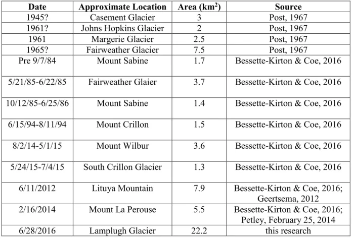
Table 2-1. Characteristics of previously documented rock avalanches travelling on ice, with areas larger than 1 km2, in Glacier Bay National Park and Preserve.
Date Approximate Location Area (km2) Source
1945? Casement Glacier 3 Post, 1967
1961? Johns Hopkins Glacier 2 Post, 1967
1961 Margerie Glacier 2.5 Post, 1967
1965? Fairweather Glacier 7.5 Post, 1967
Pre 9/7/84 Mount Sabine 1.7 Bessette-Kirton & Coe, 2016 5/21/85-6/22/85 Fairweather Glaier 3.7 Bessette-Kirton & Coe, 2016 10/12/85-6/25/86 Mount Sabine 1.4 Bessette-Kirton & Coe, 2016 6/15/94-8/11/94 Mount Crillon 1.5 Bessette-Kirton & Coe, 2016 8/2/14-5/1/15 Mount Wilbur 3.6 Bessette-Kirton & Coe, 2016 5/24/15-7/4/15 South Crillon Glacier 1.3 Bessette-Kirton & Coe, 2016 6/11/2012 Lituya Mountain 7.9 Bessette-Kirton & Coe, 2016;
Geertsema, 2012 2/16/2014 Mount La Perouse 5.5 Bessette-Kirton & Coe, 2016;
Petley, February 25, 2014
6/28/2016 Lamplugh Glacier 22.2 this research
Figure 2-2. Profile of pre-event topography along the travel path of the Lamplugh rock avalanche.
originates from a flow divide at 750 m a.s.l that is shared by the Brady and Reid Glaciers, and flows north toward Glacier Bay (Loso et al., 2011). Mass balance measurements between
1995-2011 show that the Lamplugh Glacier consistently lost mass throughout the period, with a maximum loss rate of 0.54 meters per year between 2000 and 2005 (Loso et al., 2011).
CHAPTER 3 PURPOSE
The purpose of this research is to study the emplacement mechanisms of rock avalanches travelling over ice through a case study of the Lamplugh rock avalanche in GBNP. This research will specifically focus on the volume and distribution of material within the deposit, and
structures and surficial features. Data used for this research are limited to that which can be obtained from satellite imagery. The main objectives of this research are to:
1. Demonstrate the capacity to use high-resolution satellite imagery to study rock avalanches travelling over glaciers and develop a framework for improved volume estimates and remote identification of characteristics indicative of emplacement processes.
2. Establish interpretations of emplacement dynamics through an integrated examination of volume and thickness distribution, landslide structures, and surficial features.
The following sections describe the methodologies and results relevant to each of these objectives.
CHAPTER 4 METHODS
4.1 WorldView Imagery
The WorldView-1, 2, and 3 satellites are part of the Digital Globe, Inc. constellation and have been collecting high-resolution imagery since 2007, 2009, and 2014, respectively
(DigitalGlobe, Inc., 2016b, 2016c, 2016d). The satellites in the Digital Globe constellation collect imagery in the visible light spectrum from both panchromatic and multispectral sensors. As shown in Table 4-1, there is some variation in the resolution between both sensors and specific satellites, although overall the resolution is strikingly better than many other satellites (e.g. Landsat). The panchromatic and multispectral band resolutions listed in Table 4-1 indicate the Ground Sample Distance (GSD) at 20 degrees off-nadir. This value is listed instead of the slightly better GSD at-nadir resolution because all of the imagery used in this research pertains to the former.
Table 4-1. Panchromatic and multispectral sensor resolution and geolocation accuracy of WorldView-1, 2, and 3 satellites (DigitalGlobe, Inc. 2016b, 2016c, 2016d).
Satellite Panchromatic Band
Resolution (GSD at 20° off-nadir) Multispectral Band Resolution (GSD at 20° off-nadir) WorldView-1 0.55 m n/a WorldView-2 0.52 m 2.07 m WorldView-3 0.34 m 1.38 m
In addition to traditional imagery collection, the Digital Globe constellation has the capability to collect stereo pairs from the same orbit with a time delay of approximately 60-90 seconds (Shean et al., 2016). This research will use Basic Level 1B (radiometrically and sensor-corrected) and Ortho Ready Standard (radiometrically and sensor-corrected and georectified) stereo products from WorldView-1, 2, and 3. All quantitative analyses will utilize Level 1B
imagery, and therefore only the accuracy of this type of imagery will be discussed further. The horizontal and vertical geolocation accuracies of Digital Globe products are measured as circular error at the 90th percentile (CE90) and linear error at the 90th percentile (LE90), respectively (DigitalGlobe, Inc. 2016a). These metrics indicate that at a minimum, 90 percent of the points measured have a horizontal or vertical error less than the specified CE90 or LE90 value (DigitalGlobe, Inc. 2016a). The horizontal and vertical geolocation accuracies of WorldView Basic Stereo products, without the use of ground control, are listed in
Table 4-2. It should be noted that documentation of an accuracy analysis for WorldView-3 products has not yet been released, therefore the value of CE90 listed is considered an estimate (DigitalGlobe, Inc. 2016d).
Table 4-2. Horizontal (CE90) and vertical (LE90) geolocation accuracy of WorldView-1, 2, and 3 satellites (DigitalGlobe, 2016a, 2016d).
Satellite Horizontal Geolocation Accuracy (CE90) Vertical Geolocation Accuracy (LE90) WorldView-1 4.0 m 3.7 m WorldView-2 3.5 m 3.6 m WorldView-3 3.5 m n/a 4.1.1 Acquired Imagery
Between June 2015 and November 2016, thirty WorldView stereo pairs were collected in the area of the Lamplugh rock avalanche. Many of these images are obscured by the presence of cloud cover and limited daylight during winter months. Eleven images with minimal cloud cover and reasonable image quality (Table 4-3) were acquired for processing. As noted in Table 4-3, portions of some images are covered in clouds or obscured by shadows and in nearly all cases, the full extent of the rock avalanche source area is not included in both stereo images.
Table 4-3. Dates of pre- and post-event Digital Globe, Inc. imagery acquired for DEM generation and mapping of the Lamplugh rock avalanche.
Collection Date Pre/post-event WorldView Satellite Stereo pairs used for DEM generation
Image (type) used for scarp delineation and/or deposit mapping Notes 6/19/2015 pre 2 No Scarp delineation (pan-sharpened multi-spectral)
Parts of scarp and deposit areas are covered by clouds; incomplete coverage of study
area in stereo pairs;
8/01/2015 pre 1 Yes Scarp delineation
(panchromatic)
10/02/2015 pre 1 No Scarp delineation Scarp area is shadowed.
6/15/2016 pre 1 Yes Scarp delineation
(panchromatic)
7/09/2016 post 3 No
Scarp delineation (pan-sharpened
multi-spectral)
Scarp area and parts of the deposit area are covered in clouds; incomplete coverage of
scarp in stereo pairs.
7/16/2016 post 3 Yes
Scarp delineation and deposit mapping
(pan-sharpened multi-spectral)
Scarp area is covered by clouds; incomplete coverage of
scarp in stereo pairs.
8/20/2016 post 1 No Scarp delineation
(panchromatic)
Clouds over toe of deposit; scarp area is shadowed. Note:
the control areas used for accuracy analysis are also covered by clouds so quality of
DEM could not be assessed.
8/27/2016 post 2 Yes
Scarp delineation (pan-sharpened
multi-spectral)
Thin clouds over deposit area; scarp area is shadowed.
9/27/20167 post 1 Yes (scarp area only)
Scarp delineation and deposit (scarp only) mapping (panchromatic)
Image is significantly shadowed over deposit area; scarp area is clear of clouds, but shadowed; scarp area is
covered in snow.
9/28/2016 post 3 Yes
Scarp delineation (pan-sharpened
multi-spectral)
Image is shadowed in scarp area; scarp area is covered in snow; incomplete coverage of
scarp in stereo pairs.
10/29/2016 post 3 No
Scarp delineation and deposit (scarp only) mapping
(pan-sharpened multi-spectral; scarp area
only)
Image is shadowed in scarp area and over deposit; deposit is covered in snow; incomplete
coverage of scarp in stereo pairs.
4.2 Elevation Datasets
Existing elevation data for the study area includes a 30-meter resolution DEM collected from the Shuttle Radar Topography Mission (SRTM) (U.S. Geological Survey et al., 2000) and a 5-meter resolution DEM collected through the Alaska Statewide Digital Mapping Initiative (SDMI) (Dewberry, 2013; U.S. Geological Survey, 2012). The SRTM DEM was collected in February 2000 and vertical accuracy in the Glacier Bay area is estimated to be ± 5 meters (Larsen et al., 2007). The SDMI 5-meter DEM was collected between August and September, 2012 and was created using Interferometric Synthetic Aperture Radar (IFSAR). The vertical accuracy of the SDMI DEM is 1.5 meters in areas with slopes ranging from 0 to 10 degrees and 9.0 meters in areas with slopes ranging from 10-20 degrees (Dewberry, 2013).
4.3 Ames Stereo Pipeline Workflow
The NASA Ames Stereo Pipeline (ASP) is a semi-automated, open-source
stereogrammetry software that is capable of generating DEMs from high-resolution satellite imagery (Beyer et al., 2016). ASP was originally created to process planetary imagery and has only recently been adapted for terrestrial use. The capability to process Digital Globe imagery was established to create models of ice and bare rock (Beyer et al., 2016) and functionality has only been fine-tuned for imagery of the Antarctic and Greenland ice sheets, with some test cases in Washington State and Alaska (Shean et al., 2016). ASP has functionality specific to
WorldView-1, 2, and 3 images and was used to generate high-resolution (2m) DEMs from Level 1B products. ASP Version 2.5.3 was released on October 11, 2016 and was used for all
steps: 1) image pre-processing and pre-alignment, 2) stereo correlation, and 3) raster conversion. Each processing step is discussed in detail in the following sections.
4.3.1 Pre-processing and Pre-alignment
Major sources of inaccuracy in WorldView imagery are sensor boundary artifacts, which are caused by slight offsets among all of the individual sensors within a single cluster of sensors, all of which are used to produce one complete image. ASP provides corrections for WorldView-1 and 2 images, which were applied to all applicable images during pre-processing. Artifact corrections for WorldView-3 imagery are not available in Version 2.5.3.
During pre-processing, individual image tiles from the same parent image can be mosaicked. This can reduce the number of scenes that need to be processed if more than one image tile is required to cover the study area. For most of the image sets listed in Table 4-3 the complete extent of the Lamplugh rock avalanche deposit was included in a single image tile. For the images in which this was not the case, image tiles were mosaicked prior to further
processing.
Orthorectification to a coarse (~30-meter resolution) DEM was used to pre-align stereo images to reduce the amount of time needed to search for matching points in the source images during stereo correlation. This process improves the quality of results, especially in areas of steep terrain, and eliminates the need to use an alignment algorithm during stereo correlation (Beyer et al., 2016). All images were superimposed onto a 30-meter resolution SRTM DEM.
According to the ASP User Guide a bundle adjustment process, which adjusts camera positions and orientations to be self-consistent, is recommended during pre-processing unless co-registration with ground control points is performed during post-processing (Beyer et al., 2016).
Alternatively, Shean et al. (2016) assert that this step is not necessary for WorldView-1 and 2 images because the geolocation accuracy of these satellites typically results in low triangulation error during stereo correlation. The use of bundle adjustment is recommended for triangulation errors (see Section 4.3.2) greater than one meter (O. Alexandrov, personal communication, January 30, 2017). The use of bundle adjustment on WorldView-2 and 3 images in this research resulted in a misalignment between the point cloud generated during stereo correlation and the final DEM, and in some cases produced anomalously high or low elevation values. This discrepancy could be a result of a software bug (O. Alexandrov, personal communication, January 30, 2017) or could require additional processing adjustments, which were not pursued further. Although the use of bundle adjustment was successful for WorldView-1 imagery, the triangulation error for all DEMs was found to be reasonably close to one meter. To maintain consistency in processing, a bundle adjustment was not used to produce any of the DEMs used for analysis.
4.3.2 Stereo Correlation
Image matching and triangulation are used during stereo correlation to produce a point cloud of elevation values. Initially ASP builds a disparity map by computing the x and y offsets for each matched pixel in a set of stereo pairs. This disparity map is built using normalized cross-correlation with a search window of 21 x 21 pixels (Beyer et al., 2016). The initial disparity is a first approximation, which uses only integer values. Sub-pixel refinement is used to iteratively optimize the offset of each pixel using the integer value as an initial approximation. Several refinement algorithms are available in ASP. The use of an affine adaptive Bayesian expectation-maximization algorithm (subpixel-mode 2) produces the most accurate results, but is
significantly more time intensive (Shean et al., 2016). Subpixel-mode 2 is recommended for scientific analyses and can improve results in areas with steep topography (Shean et al., 2016). Subpixel-mode 2 was used to produce all DEMs in this research.
Before triangulation, the disparity map is automatically filtered to reduce the presence of artifacts in the point cloud. During triangulation the camera models associated with each stereo pair are used to calculate elevation values for each point by reconstructing a three-dimensional location in space through the intersection of rays from each camera (Beyer et al., 2016). Image matching can be poor or fail altogether in areas with limited texture or low contrast, or in areas that are highly distorted due to different image perspectives, which is often the case in steep areas. (Beyer et al., 2016). While the absence of tree cover and vegetation and the presence of rock and ice make the study area an ideal candidate for image processing in ASP, areas of steep topography or poor lighting due to shadows or cloud cover could nevertheless cause processing blunders.
Another source of inaccuracy specific to WorldView imagery is camera jitter, which results from slight inaccuracies in the position and orientation of sensors. Low frequency camera jitter can be corrected automatically in ASP by solving for adjustments in an individual image before performing stereo correlation. This process reduces the presence of horizontal banding and was implemented on a case by case basis to improve DEM quality. Although this step improved image quality in most cases, stripping artifacts are still apparent in some DEMs and in the future, fine-tuning of this parameter could further improve quality.
4.3.3 Raster Conversion
During post-processing the point cloud of elevation values created during stereo correlation is converted to a gridded DEM that can be used with a geographic information system (GIS) platform. The output resolution of the DEM is recommended to be at least three times courser than that of the input image resolution (Beyer et al., 2016). Since Digital Globe panchromatic imagery has an input resolution of 0.5 meter, DEMs were produced with an output resolution of 2 meters. An automated filtering process was used to remove outliers larger than three times the value of the 75th percentile (Beyer et al., 2016). During triangulation, the distance between two theoretical photogrammetric rays at their closest intersection is recorded, and a map of intersection error values can be specified as an additional output during DEM generation. The intersection error can be used as a metric of relative accuracy or self-consistency, but is not representative of the absolute accuracy of a DEM (Beyer et al., 2016).
4.4 DEM Generation
One set of pre-event stereo pairs (6/15/2016) and three sets of post-event stereo pairs (7/16/2016, 8/27/2016, and 9/28/2016) were used to produce DEMs over the study area. In all of these images, the rock avalanche scarp area is covered in clouds, obscured by shadows, or does not appear in both stereo images, causing the source area to appear as a hole in the output DEMs. Improved coverage of the scarp area was identified in an additional post-event stereo pair from 9/27/2016. This set of images was used to produce a DEM over only the source area. Since the source area was not completely covered in the pre-event image acquired on 6/15/2016, a 5-meter resolution SDMI DEM was also used for pre-event coverage of the source area.
4.5 DEM Accuracy Analysis
Since vertical ground control is not available for the study area the relative accuracy of DEM pairs was assessed to establish a baseline from which to assess elevation changes between any two given dates. The relative accuracy of DEMs produced in ASP was assessed by
determining the elevation difference between stable bedrock locations in each DEM pair. Six control areas located approximately 12 kilometers north of the study area (Figure 4-1) were chosen by identifying areas of bedrock that were assumed to be stable and were not covered by snow. Control Areas 4-6 are common to the four sets of images used to produce DEMs over the deposit area. Control Areas 1-3 were used to assess the elevation difference between the post-event DEM of the source area (9/27/2016), the pre-post-event DEM from 6/15/2016, and the SDMI DEM since Control Areas 4-6 are not located in the images collected on 9/27/2016. The average slope of each control area is listed in Table 4-4. With the exception of the source area, the average slope in the control areas exceeds the range of slopes observed within the Lamplugh rock avalanche. Since vertical accuracy of DEMs is a function of slope (Tsutsui et al., 2007), it is assumed that the level of accuracy determined in the control areas will be the upper limit of elevation accuracy in the Lamplugh rock avalanche deposit.
Table 4-4. Average slope of each control area used to assess the accuracy of differenced DEMs over the Lamplugh rock avalanche.
Control Area Average Slope
1 40.4 degrees 2 40.1 degrees 3 32.0 degrees 4 32.5 degrees 5 23.1 degrees 6 23.3 degrees
Figure 4-1. Digital Globe Inc. image collected on 8/27/2016 showing the location of the six control areas used to assess the relative accuracy of DEMs produced in ASP.
DEMs of the control areas were produced in ASP and differenced DEMs corresponding to the image sets used for analyses were produced by pixel-wise subtraction. The differenced pixel values from each control area were extracted and used for statistical analyses. The chi-square goodness-of-fit test was used to test the distribution normality of differenced pixel values for each pair of images acquired on a specific date. The chi-square goodness-of-fit test checks the null hypothesis that a dataset was derived from a normal distribution at a given level of confidence. The mean of all differenced elevation values was found for each normally distributed set of differenced elevation values. Since normality cannot be assumed in all cases, an alternative method of estimating the population mean was also used in specific cases. According to the central limits theorem (CLT), the distribution of sample means obtained from random samples within a population will be normally distributed (Davis, 2002). Sampling with replacement with 10,000 replicates was used to find the distribution of sample means for non-normal distributions of differenced elevation values. The mean of this distribution, i.e. mean of the sample means, was used to determine the average elevation difference between each image pair. The standard deviation and interquartile range (IQR) of the differenced elevation distributions were found as measures of the variability in elevation difference that can be expected from processing. The IQR was used in addition to standard deviation since this measure is less sensitive to outliers and is acceptable to use with data that is not normally distributed.
4.6 DEM Differencing
The differences in elevation for each of the image sets listed in Table 4-5 were found using pixel by pixel subtraction. Table 4-5 also describes the use of each differenced DEM in further analyses.
Table 4-5. Dates and uses of differenced DEMs for analysis of the Lamplugh rock avalanche.
Dates of Differenced DEM Use of Differenced DEM
6/15/2016-7/16/2016 Shortest available time interval between pre- and post-event images; used for primary assessment of elevation changes during emplacement.
7/16/2016-8/27/2016 Post-failure changes within deposit; seasonal snow and ice change on adjacent glacier surface
8/27/2016-9/28/2016 Post-failure changes within deposit; seasonal snow and ice change on adjacent glacier surface
SDMI 5m-9/27/2016 Most complete pre- and post-event coverage in the source area; used for primary assessment of changes during emplacement.
6/15/2016-9/27/2016 Partial coverage of source area; shortest available time interval between pre- and post-event images; used for primary assessment of changes during emplacement.
4.7 Elevation Adjustments
The net snow and ice change between two dates for which stereo imagery is available can be measured by the creation and differencing of DEMs. However, the unmeasured changes in snow and ice between the acquisition of pre- or post-event imagery and the rock avalanche occurrence may be significant. The measured differences between pre- and post-event imagery are indicative of the elevation change between the actual imagery dates, but may not be an
accurate representation of surface elevations at the time of the event. To reconstruct the thickness and volume of the Lamplugh rock avalanche at the time of the event, several elevation
adjustments must be made to approximate topographic elevations directly before and after the event. The following factors were not immediately accounted for during initial DEM
differencing and required additional adjustments:
A. Snow and ice melt on the adjacent glacier surface between 6/15/2016 (date of pre-event images) and 6/28/2016 (date of rock avalanche).
B. Snow and ice melt on the adjacent glacier surface between 6/28/2016 (date of rock avalanche) and 7/16/2016 (date of post-event images).
C. Snow and ice melt in the area covered by the deposit from melting of entrained snow and ice, compaction within the deposit, and/or melting of underlying ice.
The effects of these factors cannot be directly quantified from the data that are available, but they are significant considerations for calculating deposit volume and thickness. The
following sections describe how these factors affect both positive and negative areas of the deposit. No elevation adjustments were made in the source area because most of this area consists of bedrock and is not affected by changes to the glacier surface. Three scenarios were examined: Scenario 1 takes into account the elevation loss due to A and assumes B and C are equivalent; Scenario 2 extends Scenario 1 to account for elevation loss due to B, while C is assumed to be zero; Scenario 3 replicates Scenario 2 with a nonzero value of C.
4.7.1 Scenario 1: Areas of Net Positive Elevation
The effect of melting between the acquisition of pre-event images (ti) and the rock
avalanche event (te) is represented in Figure 4-2 by a decrease in surface elevation between ti and te1 (te at time step 1). Consequently, the height at which the deposit is emplaced is lower than the surface elevation measured at ti. Additional melting between emplacement and the acquisition of post-event images (tf) is assumed to be uniform in areas covered by the deposit and areas on the adjacent surface. In Figure 4-2, the pre- and post-event surfaces that are subtracted during DEM differencing are represented by the light blue and red lines, respectively. The green arrows represent the elevation change measured in individual locations both within the deposit and on the adjacent surface. In areas covered by the deposit, the elevation difference measured between
pre- and post-event DEMs (h2) is not representative of the entire deposit thickness. If the value of h2 for every pixel over the deposit area is multiplied by pixel area, the resultant volume will not be representative of the actual deposit volume. The hachured area in
Figure 4-2 represents the volume of the deposit that is not measured. This effect is only observed when examining the vertical change between identical locations in space (pixel by pixel), as is done during DEM differencing. The change in elevation on the adjacent glacier surface between ti and tf (h1) is accurately measured by the differenced DEM. The true deposit thickness (thtrue) is therefore expressed by Equation 4-1.
Figure 4-2. Diagram showing the effect of unmeasured changes in surface elevation between the acquisition of pre-event imagery collected on 6/15/2016 and post-event imagery collected on 7/16/2016 and the occurrence of the Lamplugh rock avalanche on 6/28/2016 in deposit areas with net positive volumes. The elevation of the glacier surface at time ti (light blue line) is subtracted from the surface elevation measured at time tf (red line) during DEM differencing. The thickness of the deposit measured by DEM differencing (h2) is not equivalent to the actual thickness of the deposit (thtrue). True deposit thickness can be measured by summing the difference in elevation on the adjacent glacier surface between ti and tf (h1) with h2.
ℎ� = ℎ + ℎ Equation 4-1 ℎ � : true deposit thickness (m)
ℎ : change in elevation on the glacier surface measured by DEM differencing between ti and tf (m)
ℎ : deposit thickness measured by DEM differencing between ti and tf (m)
4.7.2 Scenario 1: Areas of Net Negative Elevation
The impact of unmeasured elevation changes from ice melt is more complex in areas of the deposit that have a net negative elevation. Scour and entrainment of surficial material is assumed to be the cause of deposit areas with a net loss in elevation between 6/15/2016 and 7/16/2016. As discussed in later sections, differential melting cannot be the cause of net negative areas within the extent of the deposit. As shown in Figure 4-3, the effects of unmeasured ice melt in net negative areas are twofold. First, the height of material that is entrained (hentrained) is
overestimated in areas within the deposit, and second, the thickness of material deposited in the scoured area (hfill) is not accounted for. Figure 4-3 shows a loss in elevation on the glacier surface between ti and te1, which is not measured by differencing of pre- and post-event DEMs. Time steps te2 and te3 show scour and entrainment of material and the subsequent deposition of material. The elevation differences in areas on the glacial surface and areas within the deposit which are measured by subtracting the elevation of the pre-event surface (light blue line) and the post-event surface (red line) are represented by h1n and h2n, respectively. If ice melt between te and tf is assumed to be the same in areas covered by deposit and on the adjacent glacier surface, hentrained is expressed by Equation 4-2.
ℎ � ���� = ℎ ���− ℎ �+ ℎ � Equation 4-2 ℎ � ���� : height of material that is scoured and entrained during emplacement (m) ℎ ���: thickness of the deposit that is emplaced in the scour area (m)
ℎ �: change in elevation on the glacier surface measured by DEM differencing between ti and tf (m)
ℎ �: height of scoured area measured by DEM differencing between ti and tf (m)
Figure 4-3. Diagram showing the effect of unmeasured changes in surface elevation between the acquisition of pre-event imagery collected on 6/15/2016 and post-event imagery collected on 7/16/2016 and the occurrence of the Lamplugh rock avalanche on 6/28/2016 in deposit areas with net negative volumes. The elevation of the glacier surface at time ti (light blue line) is subtracted from the surface elevation measured at time tf (red line) during DEM differencing. Neither the height of scoured and entrained material (hentrained) nor the height of material
deposited in the scoured area are represented by the change in elevation measured between ti and tf in areas of the deposit (h2n). Elevation change on the adjacent glacier surface between ti and tf is represented by the height of h1n. The actual thickness of entrained material can be measured by subtracting h1n from the sum of h2n and hfill.
4.7.3 Scenario 2: Areas of Net Positive Elevation
The case discussed in Scenario 1 becomes more complicated if differential melting between the area covered by debris and the surrounding glacier surface is taken into account. In this case, the deposit is assumed to prevent any ice melt in the area underlying the deposit and it is assumed that the deposit does not undergo compaction from melting of entrained snow and ice or other densification processes. Scenario 3 (below) will explore the adjustments required when there is ice melt under the deposit or compaction within the deposit. Figure 4-4 shows how differential melting affects elevation measurements made during DEM differencing. Time steps
ti, te1, and te2 are assumed to be the same as those shown in Figure 4-2. The change in elevation on the adjacent glacier surface between te and tf (h3) is shown by the purple arrow in Figure 4-4. The value of h3 cannot be directly measured from pre and post-event DEMs. With the presence of differential melting, the actual thickness of the deposit is expressed by Equation 4-3.
ℎ � = ℎ + ℎ − ℎ Equation 4-3 ℎ � : true deposit thickness (m)
ℎ : change in elevation on the glacier surface measured by DEM differencing between ti and tf (m)
ℎ : deposit thickness measured by DEM differencing between ti and tf (m) ℎ : change in elevation on the glacier surface between te and tf (m)
The sum of h1 and h2 is equivalent to the apparent thickness (thapparent) of the rock avalanche deposit on 7/16/2016 rather than the true thickness of the deposit at the time of deposition. This effect is apparent if the thickness of the deposit is observed or measured from two different locations in space (i.e. comparing the height of the deposit with the height of a location on the adjacent ice surface) rather than observing the difference from one location in space (i.e. a specific pixel in the differenced DEM).
4.7.4 Scenario 2: Areas of Net Negative Volume
The modification of Scenario 1 for areas of net negative volume to include differential melting between the adjacent surface and the deposit with the assumption that the change in elevation within the deposit is zero is shown in Figure 4-5. The change in elevation on the adjacent glacier surface between te and tf is measured by h3n. The height of entrained material is found using Equation 4-4.