VTI driving simulator : Mathematical model of a four-wheeled vehicle for simulation in real time

Nr 267A 1984 ISSN 0347-6030

26/ A

Statens vag- och tratikinstitut (VTI) +581 01 Linkoping Swedish Road & Traffic Research Institute * 8-581 01 Linkoping » Sweden

VTI Driving Simulator

Mathematical Model of a Four-wheeled Vehicle for Simulation in Real Time

Nr 267A 1984

Statens vag- och trafikinstitut (VTI) - 581 O1 Link ping

VTI Driving Simulator

2 A

Mathematical Model of a Four-wheeled

Vehicle for Simulation in Real Time

by Staffan Nordmark

CONTENTS Page ABSTRACT I REFERAT II SUMMARY III SAMMANFATTNING VI 1 INTRODUCTION 1 2 MODEL DESCRIPTION 5

3 COORDINATE SYSTEMS AND TRANSFORMATIONS 6

4 EQUATIONS OF MOTION 7

5 EXTERNAL FORCES 9

6 WHEEL DYNAMICS 13

TIRES AND SUSPENSIONS 19

7.1 Tire model 19

Aligning torque. Free rolling wheel 22 Suspension and steering compliances. 25 Effective cornering characteristics

7.4 Tire carcass elasticity 28

8 BRAKING SYSTEM 31

9 ENGINE AND DRIVE LINE 33

10 STEERING SYSTEM 38

11 ROLLING RESISTANCE AND WIND FORCES 42

12 VALIDATION 45

REFERENCES 51

LIST OF SYMBOLS 53

VTI DRIVING SIMULATOR Mathematical Model of a Four-wheeled Vehicle for Simulation in Real Time

by Staffan Nordmark

Swedish Road and Traffic Research Institute

8-581 01 LINKGPING Sweden

ABSTRACT

This report contains a theoretical model for describing the motion of a passenger car. The simulation program based on this model is used in conjunction with an

advanced driving simulator and run in real time. The

mathematical model is complete in the sense that the dynamics of the engine, transmission and steering system is described in some detail. Tire forces are given.by tabular data. Steering and suspension compliances are lumped together with the tire forces to give effective cornering characteristics. Wheel rotational equations are integrated and the associated difficulties discussed. Rolling resistance and aerodynamic forces are included to some extent. The model is validated during transient manoeuvres and the results correspond well with field test data.

II

VTI KGRSIMULATOR - Matematisk modell av ett fyrhjuligt fordon for realtidssimulering

av Staffan Nordmark

Statens vég- ochtrafikinstitut

581 O1 LINKUPING

REFERAT

Denna rapport innehéller en teoretisk modell som be-skriver en bils.rorelse. Det simuleringsprOgram, som grundar Sig pa denna modell, anvands 1 en avancerad

korsimhlator och kors alltsé i realtid. Den matematiska

modellen beskriver aven motorns, transmissionens och

styrningens egenskaper detaljerat. Déckskrafterna ges av tabellerade vérden. Styrningens och hjulupphéngning ens elasticiteter kopplas ihop med décket och ger en resulterande sidkraftkarakteristik. Hjulens rotations-ekvationer integreras och svérigheterna darvidlag disku-teras. Rullmotsténd och luftkrafter ér medtagna i Viss utstréckning. Modellen ér validerad under transienta manovrer och resultaten overensstémmer Val med falt-experiment.

III

VTI DRIVING SIMULATOR - Mathematical Model of a Four-wheeled Vehicle for Simulation in Real Time

by Staffan Nordmark

Swedish Road and Traffic Research Institute

8-581 01 LINKGPING Sweden

SUMMARY

This report describes the mathematical model of a paSsenger car that is currently used in an advanced driving simulator at the Swedish Road and Traffic

Research Institute.

The basic model describes a four-wheeled vehicle with freedom to move in the plane and to yaw. Neither roll nor pitch are included but a semistatic load transfer between the wheels is used. The distribution of this

load transfer is specified among the input data thus obtaining some of the effects of different spring lay-outs. This is very important since the horizontal tire forces depend on the vertical load in a nonlinear

manner .

The difficulties to integrate the rotational equations of motion for the wheels are discussed especially when the time-step is comparatively long. One approximate solution to this problem is described.

The horizontal tire forces are.given as tabular data and depend on the vertical load, slip angle and longi-tudinal slip. Intermediate values are computed by linear interpolation and it is assumed that the functions can be factorized in a special way.

Simple analytical tire models have been tried, but

these tend to give a coupling too strong between lateral and longitudinal forces. This will result in exaggerat ing the difference between front and rear driven cars.

IV

It is not only the tire cornerning characteristics that determine the handling qualities of car. The suspensions and steering system will add compliance to the tires thus influencing the overall cornering stiffness. We have chosen to use the concept of effective cornering characteristics i.e.these compliances are lumped

together with that of the tire. This procedure is

described in detail.

Due to tire carcass elasticity the contact patch between tire and ground will move relatively the wheel center. This will induce torques on the vehicle mass as well as changes in steering angles and is in fact the main reason for the tendency of vehicles to tuck inwards a curve when the throttle is released. These effects

are for that reason included in the model.

The braking system has as Option a reduction valve coupled to the brakes of the rear wheels.

The engine and driveline are also described in some detail. A simple but effective algorithm is given for the complex relationship between throttle, engine torque and engine speed. The most important qualities of the final drive with differential is included dividing the torque equally between the wheels and coupling the

moment of inertia of the flywheel to that of the wheels.

The reaction torque at the steering wheel is computed for small steer angles but the effects of inclinations of the steering axis are considered in detail. Some Coulomb damping is included and hysteresis effects is obtained by first order filtering of the damping.

Rolling resistance of the wheels are introduced at each wheel and aerodynamic drag prOportional to the square of velocity is used to maximize the speed. Side wind

and wind gusts perpendicular to the vehicle trajectory are also given in equation form. These can be used as surprise elements to a driver in the simulator.

VI

VTI KGRSIMULATOR - Matematisk modell av ett fyrhjuligt fordon for realtidssimulering

av Staffan Nordmark

Statens vag- och trafikinstitUt

581 O1 LINKoPING Sweden

SAMMANFATTNING

Denna rapport beskriver det teoretiska underlaget till ett program som beskriver kordynamiken hos en

personbil. Detta program anvands i en avancerad kor

simulator som for narvarande ar i bruk Vid Statens vag- och trafikinstitut (VTI).

I princip beskrivs med ekvationer rorelsen hos ett fordon med fyra hjul som kan rora sig pa ett plan i alla riktningar samt vrida sig runt en vertikalaxel

(girrorelse). Varken krang eller tipprorelse beaktas

men den lastoverflyttning mellan hjulen som sker p g a

accelerationer ar medraknad genom ett "semistatiskt" betraktelsesatt. Lastoverflyttningen i sidled forde

las mellan fram och bakaxel i proportionen som anges som indata till programmet. Pa detta satt kan olika val av krangstyvheter fram- bak simuleras. Detta ar mycket viktigt eftersom de horisontella dackskraf terna i allmanhet ar olinjara funktioner av vertikal belastningen.

Svarigheterna da det galler att integrera rotations-ekvationerna for hjulen diskuteras och speciellt fallet med ett relativt sett langt tidssteg. En approximativ losning till detta problem ar angiven.

De horisontella dackskrafterna ges som tabellvarden och ar funktioner av vertikalbelastning, avdrifts-vinkel och longitudinellt slip. Mellanliggande

var-den beraknas med linjar interpolation och som forenkling

VII

antas att funktionerna kan faktoriseras pa ett speci

ellt satt.

Enkla analytiska modeller for dackskrafterna har pro

vats, men dessa tenderar att ha en alltfor stark

kOppling mellan sid och langskraft. Detta leder till

att overdriva skillnaderna mellan fram och

bakhjuls-drivna bilar.

Det ar inte bara dackens sidkraftkarakteristika som bestammer ett fordons koregenskaper. Fjadersystemet

och styrningen ar ofta eftergivlig da man lagger pa

en sidkraft och paverkar pa detta satt den sammanlagda sidkraftskoefficienten. Vi har valt att arbeta med sadana resulterande sidkraftskarakteristika dar dessa eftergivligheter adderas till dacket sjalvt. Denna metod beskrivs i detalj.

Pa grund av dackets och framfor allt dacksidans mjuk-het kommer kontaktytan mellan dack och vagbana att

forskjutas fran en punkt under hjulcentrum. Detta gor

att speciellt de longitudinella krafterna kommer att utova ett (aterstallande) moment pa fordonet under kurvtagning. Detta ar den framsta orsaken till 55 kallade g us-slapp reaktioner i kurva. Vidare kan dessa moment orsaka forandrade styrvinklar vilket pa verkar beteendet under sadana manovrer. Av denna an-ledning ar dessa effekter behandlade i modellen.

Bromssystemet ar i huvudsak en proportionell overfo-ring av pedalkraft till bromsmoment. Mojligheten av

en tryckreduceringsventil till bakaxeln finns dock

med.

Motorn och kraftoverforingen beskrivs ganska detalje-rat. En enkel men anvandbar algoritm anges for det komplicerade sambandet mellan gaspadrag, vridmoment

VIII

och varvtal. De Viktigaste egenskaperna hos differen-tialen finns med sésom att momentet fordelas lika mellan drivhjulen och att svénghjulets troghetsmoment adderas till drthjulens.

Reaktionsmomentet i ratten ar beréknat for smé styr-Vinklar men hénsyn har tagits till styraxlarnas lut-ning i olika riktlut-ningar. Coulomb-friktion r inlagt i styrsystemet och for att éstadkomma hysteres dam-pas denna signal med ett forsta ordningens filter.

Rullmotsténd proportionellt mot vertikalbelastningen ér inlagt vid varje hjul. Fordonets maximala hastig het begrénsas av luftmotsténdet som ér proportionellt mot kvadraten p5 hastigheten. Likasé finns mojlighet att légga in sidvind eller vindbyar rakt frén sidan. Dessa kan anvandas som overraskningsmoment for en

fo-rare 1 simulatorn.

INTRODUCTION

This report describes the mathematical model of a passenger car that is currently used in an advanced driving simulator at the Swedish Road and Traffic

Research Institute (VTI).

The plans for building a simulator at VTI can be traced back to the sixties but first in 1978 the financial support from the National Swedish Board for Technical Development made it possible to build such a system. Different versions of the simulator

have been in operation during these years. The develop-ment stages have spanned from only a chair and steering wheel standing on the floor with a simple oscilloscope

picture to the moving base simulator with wide angle

visual system that is used today. An important step in the development was taken during the spring 1983 when it was possible to drive the simulator with the complete moving base system for the first time. There is of course room for improvements and the development

will continue.

The current version is equipped with a moving base system for simulating inertia forces. The design and general lay-out of the simulator is of course inSpired by existing simulators elsewhere and most notably the

one at VW-Werk. The VW-simulator [12] works with

rotations of the cabin (roll, pitch and yaw) where

the basic idea is to use a component of the gravita

tional acceleration to simulate accelerations in

different directions. The VTI-system also has three

degrees of freedom but the yaw motion has been cancelled in favour of pure lateral motion along rails. See

figure 1.1.

The lateral inertia forces can thus be simulated both

by giving the cabin a specified roll angle and by

lateral acceleration. These two principles are combined to use the roll mainly for constant accelerations as

in a curve while lateral motion is used for manoeuvres on straight roads. The longitudinal accelerations are

simulated only by giving the cabin a suitable pitch angle.

Figure LgLGeneral lay out of driving simulator with moving base system

All the motions are Operated by hydraulic engines via chains and the hydraulic system is dime

nsioned for

simulating accelerations up to 0.4 g. This means that some scaling of accelerations must be used when driving on high friction surfaces.

The vision field is produced by three colour TV-projectors mounted above the driver s he

ad and the

screens are situated in front of the head at

approxi-mately a distance of two metres from the eyes of the

driver. The road picture is generated purely by

electronics developed at VTI and consists of different kinds of roads and surroundings. The horizontal and vertical curvature can be continuously varied and several objects (signs, obstacles etc) be introduced.

This report will describe in detail the mathematical model that is used for describing the vehicle and

its motion. This is an out growth of an earlier attempt described in [1Q]. That report was written

to form a base for program construction at the initial

development phase. At that time a hybrid computer was available and most parts of the model.weresuccessfully programmed.

The important friction forces between tires and ground werenmdelled by using simple analytical expressions as derived in [2]. Experiments in an early fixed-base simulator indicated a qualitatively correct

behaviour of the vehicle but there was certainly

room for improvements. Specially it was felt that traction and braking forces influenced the handling

qualities too much and it was hard to obtain a normal degree of understeer without lowering the cornering stiffness at the front.

Based on these experiences a fairly large revision was carried out. The friction forces between tire and ground were now given in tabular form using linear interpolation and suSpension and steering

system compliances were included in the tire model by computing the effective cornering characteristics.

Since the program must run in real time there is a limit in model complexity determined by the available

computer and the time step used. We have chosen not to describe the vertical working of suspensions and sprung mass motion, but rather concentrate on the representation of tire forces and steering effects in suspensions. Comparisons with field test data have supported this approach. Very good agreement has been reached between field test data and results from the computer when studying the transient behaviour of a passenger car performing lane change manoeuvres with different severity and rapidness.

The program is written in FORTRAN 77 and run on a SEL 32/57. The cycle time (time available to exchange data between cabin and computer and run through the computer program once) is 20 ms and today is 12 ms used. This is valid for the complete program including parts governing the motion of the moving base system .and the visual system besides the vehicle dynamics.

Naturally a simulation model is a mixture of parts from different sources. We have tried to state the origins of different ideas when possible. The people involved in this project have all contributed to this report to some extent. This is specially valid for Mats Lidstrom who has programmed several of the earlier versions of the simulator program. He has

also constructed the very effective model of the engine

characteristics.

MODEL DESCRIPTION

The vehicle is modelled as a stiff box with four wheels moving on a flat surface. Essentially this means a system with three degrees of freedom: linear motion in the plane and yaw. The sprung mass is neither alloWed to roll nor pitch. However, load transfer bet-ween the wheels is used, in a semi-static fashion to

simulate the effects of different suspension layouts.

The greatest effort has been spent to give a careful description of the friction forces between tire and ground. Compliances in the steering system and sus-pensions are considered as far as their influence on handling qualities are concerned.

For this model the following equations are given which are described in detail in the following sections

a) Equations of motion for the vehicle in the plane b) Rotational dynamics of the wheels

c) Engine and driveline

d) Tire model giving horizontal forces and torques

between tire and ground

e) Steering system

COORDINATE SYSTEMS AND TRANSFORMATIONS

In the sequel the following coordinate systems are

used

a) (Q X Y Z) A groundfixed system with Z- axle pointing upward

b) (G x' y' z') A system with the axles parallell

with (XYZ) and origin G in the centre

of the vehicle

a) (G x y z) _The system (Gx'y'z') rotated the angle w around the z'- axle.

For the transformation of a vector 5 between the systems

b) and c) we have the following expression

(a) = A(E)'

where A is the orthogonal transformation matrix

Icos w sin w 0

A = -sin w cos w 0 y

0 O 1

Figure 3.1 The orientation of the coordinate systems mentioned in section 3.

EQUATIONS OF MOTION

Written in vector form the equation for the planar motion of the vehicle centre of gravity is

m x = Fe (4.1)

It is natural to express this equation in the body fixed (G x y z)- system since the lateral and longi tudinal speeds have an easy interpretation in this

case .

The speed is thus

L u

X = v 0

in the (G x y z)- system which is rotating with the angular speed

The equation (4.1) can then be expressed as

at + mo x x ) = Fe

B

I

and in component form

m( u - v r) = (F )

II 33:

m(v+ur)

Transformation to landscape coordinates is carried out by

i u u cos w - v sin w

Y = At = u sin w + v cos w

0 O 0

Here the yaw angle w is integrated from the equation

I 12:65)

with suitable initial values.

The main problem is to express the external forces Fe

and moments Me in the state variables used. This will

be dealt with in the following sections.

EXTERNAL FORCES

The external forces which act upon the vehicle are in this model

1. Tire friction forces and moments

2. Wind forces and moments

The tire friction forces generally are functions

F = F(d, S, F2)

The dependance of the vertical load FZ is important

and hence a semi-static load transfer is used

h h _ F :F .F o 0F) 21 281 2% ( e)x pF tW12 ( e y

_

_.1_1_.

.h

The constants _{p F} and pR decide how the rolling torque

is distributed between front and rear axles and

corre-spond to different roll stiffnesses. Further we have the following relationship

It remains to express a and S in the state variables. The wheel hub velocity is obtained from

u - nir

E. = E + w_{l 0} x _pl. = _V + _£1.r 0

10

and this is expressed in the wheel coordinate system

by

Bl = *sin 61 cos 6. O

The slip angle di is defined by

V. d.₁ = arctan( i )_ui

and the longitudinal slip Si by R Q.1

i _u.1

where 91 is the rotational speed of the wheel, which must be computed by solving the rotational equation of

of motion for each wheel. This will be dealt with in

a proceeding section.

Thus in principle it is possible to obtain the tire forces and moments from the state variables. These are expressed in the wheel coordinate system and transformed to the vehicle system.

Finally we obtain

(Fe)y = i Fwiy + FLy (5.2)

(Fe)x = i Fwix + FLx (5'3)

( )=ZM.+Z( .F. n,F.)+M

(5.4)

11

L<

A

3:

,

Figure 5.1 Positive directions of steer angles

and velocities.

Wheel number indices.

12

V

\

\

\

\

\

\

\

Figure 5.2 Positive directions of steer angle_{. .} 5._i Sllp angle mi and Side force Fyi

13

WHEEL DYNAMICS

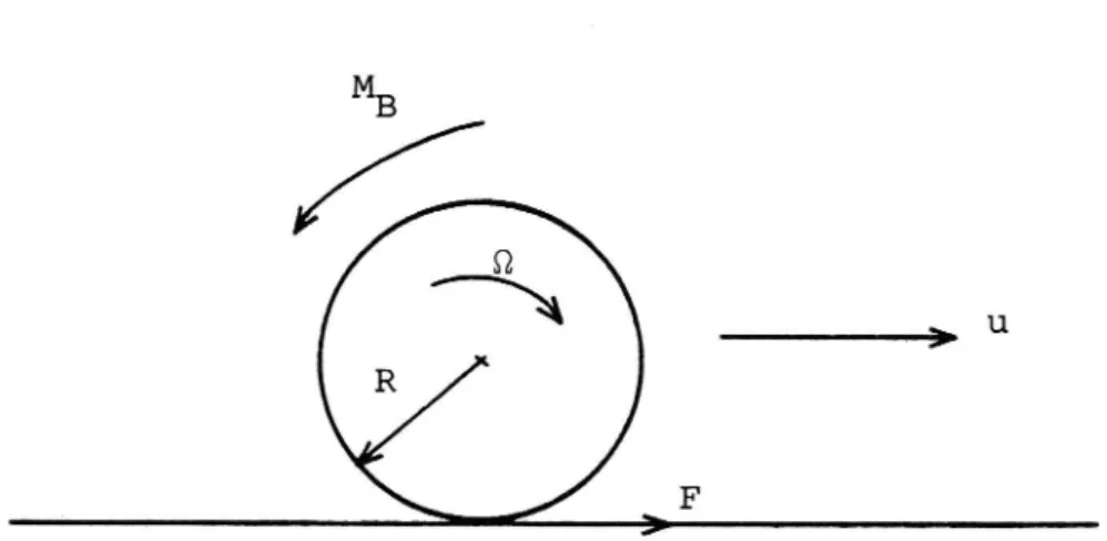
A major problem when simulating rolling vehicles is to integrate the rotational equations of motion. This is due to the behaviour of the reaction force between tyre and road when applying braking or driving torque at the wheel axle. In this section we will concentrate on this problem and calculate the timestep necessary to get an accurate description of the time history. We consider first a rolling wheel according to figure 6.1.

The subscript i" to denote wheel no "i" has been drOpped in this section to make the equations more

readable.

Figure 6.1 Positive directions of forces and

speeds in the wheel rotation equations.

The braking torque MB is applied at the axle O. The reaction force F is a function of the slip S according to the schematic figure 6.2.

14

-F(S)

:

#

>

0.5 1.0 S

Figure 6.2 Schematic representation of the longitudinal force as a function of slip.

Here the slip is defined by

(6.1)

The rotational equation of motion for the wheel is then

153 = M - R - F(S)

(6.2)

A change of variables and differentiation of (5.1) give

Vkamakethe simplifying assumption that the change of Q

is large compared to that of u. Then approximately

s=- § 2

(6.3)

15

and (6.3) in (6.2) gives

S = (M + R - F(S)) (6.4)

We simplify further by considering the first order expansion of F(S)

_ dF

F(s>

F(so) + d8 (so)

(5 so)

For each timestep we shall thus solve the initial value problem

- - O g-F O

S - uI (MB + R F(SO) + R dS(SO) (S 80))

S(O)==SO

We simplify the notation by assuming S0 = 0 and

setting F(SO) = F dF _ _

d§(so)

Cs

_{l _}

₁

_{_§}

_(6.5)

S+TS

T-CSER+F1

T=12'u

_(6.6)

Assuming that CS, MB and T are constant during the time-step it is easy to write down the exact solution. However equation (6.5) is actually only a first order

16

filter with time-constant T. For a passenger car driving at medium speed.normal values are

1 kgm2 20 m/s

0.3 m

S==6O OOO N/unit slip

O ' J U C J H II

This will give

T 2 4 ms

In the simulator the time-step used is actually 20 ms. One could of c0urse use a much shorter time-step in the slip equations but this will increase the total program time, getting it into the neighbourhood of the

absolute limit 20 ms.

Very little information is to gain by taking the wheel moment of inertia into account when CS is high. This is the case in the elastic region of the force slip curve i.e. for small slip values.

The considerations above have led to the following approach in the simulator program. The slip region is

divided into two parts, I and II. See figure 6.3.

17 -F(S) II

l

L__

l

l

l

I

|

l

l

l

l

l

I

_i

₉

regions I and II with different methods

of solving the rotational equation of motion.

It is necessary that H = -F(S) is strictly monotonous in region I thus ensuring the existence of the

. . -1

inverse function H .

In region II there might occur two kinds of singu-larities: C5 = O and/or u = O. The first case is

avoided by Maclaurin-expansion of the solution Operator to (6.5) giving the result for small values of CS.

r.

1

#35 MB

-C -(1-e rpm-3+1?)

[cslze

AS=S-S =<

(6.7)

O

_{Lf- J (Tf LF)}

RZ-At MB

_{lcs' < 8}

In the second case we simply use

I - u

T = ~ for u < u

0

18

The strategy is then quite clear. Assume that Sn

has been computed. Then if

S 63 I_n

A. S G

' n+1 R

where G is defined in both I and II by linear extension of H_1 into region II

S 65 II_n

B Sn+1 = Sn + AS

where AS is computed according to (6.7).

If then the new Sn+1 E I this value is

neglected and instead computed according to A.

19

TIRES AND SUSPENSIONS. Tire model

The applications of the simulator are very general.

They may vary from normal driving during extended periods to severe manoeuvres on low friction. It is essential that the friction forces during cornering and braking are reproduced as accurately as possible. All these demands point to a fairly complex represen-tation of tire data. Generally the friction forces

are functions FX = FX (a, 8. F2, Y) FY = FY (0"! Sr FZI Y)

S = longitudinal slip

with a nonlinear dependence on the different variables. There are two possible approaches here. One can try to find analytical expressions with only a few input data, such as cornering stiffness, peak friction

value etc. The most commonly used model of this kind

is due to Dugoff et.alJ [:2] and is described in an earlier VTI- report [10].

This model is able to give a qualitatively and in some respects quantitatively correct description of the complex interaction between longitudinal and lateral forces. The tire forces as well as the aligning torque are given as explicit functions of the slip angle, the longitudinal slip and the vertical load. These

20

functions are derived from the assumption of a certain distribution (constant and parabolic have been tried)

of the vertical load over the contact area. To get a

better correspondence with actual tire data the cor-nering stiffness and the peak lateral friction number may vary as second order polynomials of the vertical load. The coefficients of these polynomials can be

directly obtained from the extensive tire investigation

performed by Calspan [ Z].

Theoretical models of this type have been used in the

simulator for some time giving good results [331. How

ever, the coupling between lateral and lOngitudinal forces seems to be too strong, which will exaggerate over-understeering characteristics for rear and front

driven cars respectively. This oversensitivity for

traction and braking forces can be seen when comparing

tire-data from the Swedish ESV-program [341 with those obtained with Dugoff's equations. In our opinion these analytical expressions must be used very carefully, especially when stability questions arise. They will be very useful as long as qualitative studies are sufficient and program economy is an important matter. It is always possible to model a car with reasonable behaviour using such a simple analytical tire model, but for strict vehicle handling studies something better

is needed.

The other approach is to resort to experimentally measured data and interpolate between these. The draw back here is that a very substantial set of data has to be measured and put into the program. These data can also be hard to find, because values for combined cornering and braking are scarce in the literature. Further, the procedure of interpolating between tables describing functions of several variables can be time consuming, which is disadvantageous when working with

21

a real time program.

Despite this we have found a matrix or tabular

formulation worthwhile. Some simplifications have been introduced and our approach is very similar to that

in £3].

To avoid dealing with 3- dimensional matrices the following factorizations are assumed

"G_y (F_z I 0L) ' g_yred (0"!

Fy(d, S, FZ)

Fx(a, S, FZ) HX(Fz)-GX(S)-g_xred (s, a) (7.2)

The minus-sign is only a consequence of the Sign con ventions and a wish to keep the different functions in the right hand sides positive for positive arguments.

All the factors are scalar functions of respective

variables. Gy, gyred , gxred and Gx are defined on pointsets where intermediate values are computed by linear interpolation. The gxred, gyred and HX functions are normalized in the sense that

nged(a O) z gxred(S 0) = 1

H (F ) = 1 for F = F .

x z z z, nominal

This will in effect mean that Gy(Fz, d) are the side-force - slip angle curves at zero longitudinal side-force for different forces. Similar arguments are valid for GX(S).

In the simulator program the following point sets have been used. They are considered to give a reasonable resolution of the actual curves but still are possible to use in real time applications.

22

G? (Fz, d) : ( 5 x 6)

gyred (a, S) : ( 6 x 6)

GX (S) : ( 6 )

g_xred (S.oc):(6x6)

For the function Hx is assumed a simple linear dependence

H_x (F ) = F_{z z} / F_z,nominal

The tire force functions are extendedtx>negative

values of d and S by

F

(-oc, S,F)

Aligning torque. Free rolling wheel

When a free rolling wheel is forced to move at a certain slip angle a reaction force is produced at the contact patch. In the forward, adhesion region no sliding occurs and the force is built up by elastic

deformation of tread elements. In the rear, nonadhesion

region the friction force limit is reached with sliding

as a consequence. This will meanthat the resultant

is positioned behind the centre of the contact area. This can be expressed as a torque, the aligning torque,

23

or as a moment arm, the tire caster. We use a simple

expression for the aligning torque taken from [111.

MAZO = (K1 o FZ + K2 - |Fy]) - Fy

(7.3)

Equation (7.3) is probably the simplest expression that will reproduce the most important qualities of

MAZ'

maximum and then decrease to almost zero, when total

This is expected to grow for increasing Fy to a

sliding occurs over the contact area. The term K1 - F2 represents of course the tire caster or pneumatic trail. The magnitude of K2 can also be estimated by observing that

MAZO

O

for IFy] z u - F

which would implicate

o =

The aligning torque is very importantfor the handling

of the vehicle. A suspension may be designed with a small caster offset. The tire caster must then be added to this to give the total moment arm for the lateral force. Almost all suspensions are fixed to the sprung mass with elastic bushings. The resulting torque from the tire forces may deflect the suspension and add or subtract steering angles. The effect is that the system tire-wheel suspension may exhibit quite different lateral force-slip angle curves than the tire itself. The handling qualities are a

consequence of the balance between the effective cornering coefficients at the front and the rear. The steering system has usually relatively high

compliance which is a decisive factor for the

24

steering characteristic of a given vehicle.

It could be enlightening at this point to study the relative importance of these factors. Jaksch has

published several reports [6, 7], where first order

expressions have been given for the overall compliance. Using his values for Volvo 760 the total compliance at the front axle is composed of the following

contributions:

1. The tires: 64%

2. Steering compliance: 31,7%

3. Roll-steer and camber: 4,3%

4. SuSpension complianCe: 0%

That the influence from suspension compliance is nil depends on the fact that the side force vector has zero moment arm in this special case. The pneumatic trail and the suspension moment arm eliminate each other. However, at larger side forces the pneumatic trail will decrease and then the suspension compliance will have some effect on the total compliance.

With the same argument it will turn out that the steering compliance will contribute less at higher sideforces. In this region nonlinear effects will tend to play a role. The vertical load sensitivity of the tires is most important of these. The use of a stiff roll stabilizer at the front is a deliberate step of the vehicle designer to increase the under-steering tendency especially at the limit.

25

SuSpension and steering compliances. Effective cornering characteristics

A simple way to account for the compliances in the steering system and the suspensions is to couple them to the tire characteristics. This has the same effect as connecting a number of springs in series. We follow

the same procedure here as outlined by Pacejka in [11].

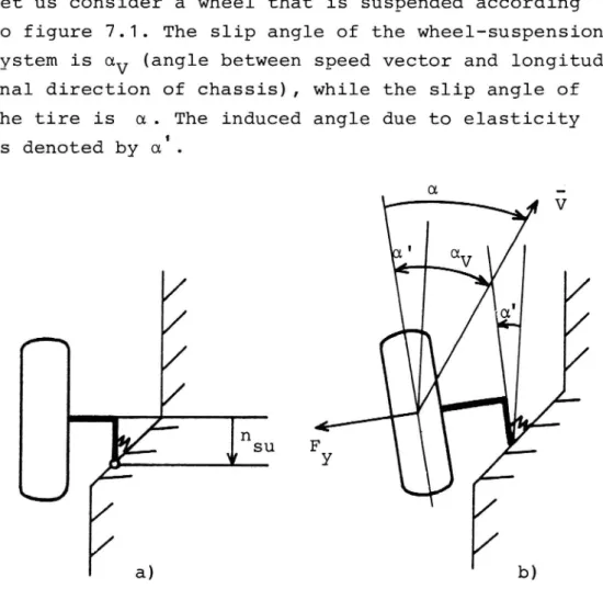
Let us consider a wheel that is suspended according to figure 7.1. The slip angle of the wheel-suspension! system is av (angle between speed vector and longitud-inal direction of chassis), while the slip angle of the tire is d. The induced angle due to elasticity is denoted by d .

\

\

\

\

a)

Figure 7.1 Effect of suspension compliance.

a) Straight driving _

b) Wheel working in direction defined by V

26

Then

where

d' = F_y - n _su - C_su

If we also consider the change in position of Fy due to the pneumatic trail A

where A is obtained from (7.3)

= 1

A ILAZO/Fy

Exactly the same reasoning can be carried out for the steering compliance. The moment arm is then defined by the caster offset and the pneumatic trail. The steering axis is denoted by O and is fixed in the suspension arms, which in turn will flex the angle

d". Then

a = -(nC + A) Fy ' CSt

where the steering compliance CS_t is measured around the point 0.

27

V

Y

Figure 7.2 Effect of steering system compliance

4% :0

Finally

a = av + a' + a" =

= av + Fy ° [nsu - Csu

nC Cst

-- A -- (csu + cst

(7.4)

The effective cornering characteristic is now computed by a shift in the FY - a curve. For given F we have from (7.4).

av = a + G(Fy)

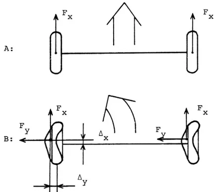
28 d I G(FY) Q 4y. .. __ _ q ) -_ -Q <

Figure 7.3 Construction of effective cornering

characteristics

A: Tire characteristics

B: Tire-suspension characteristics due to different compliances

Tire carcass elasticity

In the previous section we pointed out the importance of the aligning torque for the handling qualities. However, the expression (7.3) is only valid for a free-rolling wheel with only lateral force applied. When traction and/or braking forces also exist the contact area will be displaced due to carcass

elasticity. This effect is not neglectable and is one of the reasons for the tendency of a vehicle to tuck inwards when the throttle is released in a curve. The explanation for this is quite simple according to figure 7.4.

29

The formulation here follows Pacejka [3, p. 794

798]

but is simplified by neglecting the vertical torsional compliance of the tire.

Figure 7.4 Displacements of contact area due to carcass elasticity.

A: Straight driving B: Cornering

From the figure it is clear that both Fx and Fy will produce torques with moment arms AV and AX respectively.

ul-Introducing the tire compliances Ctx and Cty in each direction we obtain for the aligning torque (one wheel only)

MAZ = MAZO - FX - Ay + FY - AX =

= MAZO - Fx Fy Cty + FY FX - Ctx =

= MAZO + FX - Fy (CtX - Cty) (7.5)

30

Since CtX normally is less than CtV the effect of traction forces is understeering both for front and rear driven cars. It is also quite clear that the changed torques can induce steering angles due to compliances. These are taken care of by assuming

proportionality to the correction term in (7.5). Thus

A6 = FX - FY (ctx - cty) CM

(7.6)

CM is here the total compliance of the suspension and steering system per wheel.

31

BRAKING SYSTEM

The braking torque applied at each wheel is in prin ciple prOportional to the signal from a transducer in the hydraulic braking system which in part is retained in the cabin from the original passenger car. No

attempt has been made to model time delays but the

option of a pressure reduction valve to the rear wheels exists. The force at the brake pedal Bped is

trans-formed into line pressures Pf to the front and Pr to

the rear according to figure 8.1

Pknee *7

ped

Figure 8.1 Diagram showing effect of line pressure reduction valve to rear wheels

32

The equations for the line pressures are as follows:

Pf '-" Bped°BRC1

Pr = Pk

nee

Pknee+BRC2°(B ed't ~ - ); Pr>P

p

BRC1

knee

These pressures are multiplied with constants to give the braking torque at each individual wheel

M

Bi

Pf BRTi

1

1,2

M

Uneven brake distributions can thus be simulated by changing the constants BRTi.

33

ENGINE AND DRIVE LINE

The engine characteristics are described by torque

(ME) - engine speed (9E) curves for different throttle positions. The used curves are depicted in figure 9.1

and they are constructed in the following way. The throttle position is determined by the normalized variable XE (12XE20), where XE = 1 means no throttle and XE = 0 full throttle. Starting from the torque-engine speed curve

ME = f(QE); XE = O

for full throttle, the curves for XE f O are computed

by the following equations: 2

Q

E

Q

QE+ EC X

fm') MEC°XE2

Essentially this is a translation along a straight line of the curve for XE = 0 and the meaning of REC and MEC is clear from figure 9.1. This algorithm gives a good fit to experimental "performance fields" and a natural feel of the engine when driving the simulator while still fulfilling the demand of short computation time.

The engine model has also been validated by Godthelp et al [5] using an instrumented car. By suitable choice of the parameters MEC and QEC it has been possible to obtain good correspondence between mea-sured values and those predicted by the model.

34

180

-_

1/

\q<3 I

:f\\\\

0.9

10.

8

0.7

9E

T

:

.

a

4

0

100

200

3abq\4ooo\3ggo son rpm

105

209

314 419

4 628 rad/S

Figure 9.1 Engine torque versus rotational speed for

different throttle positions

The rest of the driveline is separated in different blocks. 35

WE

WD 52E

n29":

1 2

:2 9T, MT

Wj

VTI REPORT 267A

End gear Gear ratio: 2 1 6 ' u. .

-Dj

Driveline with engine gearbox, end gear and wheels

M

xi

36

For the wheels the following equations are valid

Iwi mi - MDi-MBi-in'R

(9.1)

-M .-F -°R

ij Qj = MDj B] X]

The end gear has the property of distributing the torque from the driveshaft in equal ratio

M_Di M . = §nD M_{Dj T (9'2)}

1

Q_T. inD (Qi+Qj) (9.3)

The engine has the following equation of motion

I

_{E E}

_{E c1}

_(9'4)

and for the gear box the following relations are

valid when the clutch is closed

_ 1

.

Q = 1 Q _{(9 6)}

E n₁ T °

Elimination between equations (9.1) - (9.6) will give

for wheel 1 o 2._{ng IE)Qi+ZnD n£ IEQj}' 1 2, 2. ' = U N 1 (Iwi+Zn

= 'MBi_in'R+% nD'n2°ME

(9 7)

and a similar expression (9.8) for the other wheel. The rotations of the wheels are coupled by the engine-flywheel moment of inertia.

Numerically it has proved to be difficult to solve the equations (9.7-8). Instability has occurred when

37

considering the Qj-term as a torque in the right hand side of (9.7). This is probably due to the long time-step used and the fact that the coefficient matrix of (Qi, éj) has a determinant near zero making the system (9.7) and (9.8) sensitive to disturbances. The question needs further clarification but this is not carried out

in this context.

To avoid the difficulty we have chosen to decouple the equations (9.7) - (9.8) by exchanging the coupling

term Qj for Qi in (9.7) and similarly in (9.8).

The equations are then easy to solve using the proce dure outlined earlier. In the program the drive shaft speed QT is then determined by (9.3). In this way the main results of the differential are retained and are

in fact correct when the wheels move synchronously.

10

38

STEERING SYSTEM

In the preceding chapters we have given a complete description of the dynamics of the vehicle in the

sense that the motion of the vehicle is determined

if the initial conditions and certain control variables are specified. These variables are controlled by the

driver and are as follows: . Angle of steering wheel

Brake Throttle Gear . Clutch m a c a w-a

The steer angle is transmitted from the steering wheel to the front wheels via the steering system. It is a well known fact that the driver receives a lot of in-formation concerning the road and the manoeuvre

("road feeling") from the reaction torque at the steering wheel. This feedback mechanism is thus im-portant to model rather carefully. Most parts of this have already been presented in this report. The align-ing torque as well as the tire forces were introduced in section 7 and the compliance of the steering system has already been included in the tire data. The

resulting torque at the tires is then transmitted to

the steering wheel through the steering gear with ratio ns. Some damping and friction forces are also included. Most of the expressions used are linear for simplicity but more complex representations are

possible if the need would arise. We use mainly

equa-tions derived in [9, p. 439] for the effects of caster

and kingg 11offsets. The derivation is rather lengthy

and the reader is referred to [9] for all details. We

have chosen to consider the case that the braking and tractive torques are taken up by the steering axis

39

rather than by a drive shaft coupled to the engine.

Due to the orientation of the steering axis the tire forces will create a torque at the steering wheel. The

steering axis is inclined and situated at a certain

distance from the wheel plane. These angles and dis tances are defined in figure 10.1.

Steering axis F" 1 \ ,I

t \

_\

_R

_I

\

nC

l

lro

Figure 10.1 Front wheel seen from the side and from

the rear. 0 caster angle caster offset ni II II nc 6 = kinggnxlinclination r0 = kingg mloffset

It is now possible to express the combined torque MR from both sides assuming that the geometrical data are

the same for both sides. Then, for small steer angle 6 MR = (FX2 - FX1)-r0 - (FY1 + Fy2)°nC

+(F22 _ F21).a1 +(Fx1 + Fx2).6.a2

+(Fy2 - Fy1) c3°a3

_(Fz1 + F22).6.a4 + MAZ1 + MAZZ

40

where

a1 = rotanI + nctano

a2 = tang-(ro tanT + notano)

a3 = rO'tanZT + notanT tang + R'tano

: I .

a4 r0 tang nctanT

with

r0' = r0 + R-tanc nO = nC - R°tanT

and MAz1, MAZ2 are the complete expreSSions for the aligning torques as given in section 7.4.

Some damping is also included in the system. This has mainly the form of Coulomb friction to give hysteresis

effects. See figure 10.2

A MSWD

MSWDM -

'-0

9

0

Figure 10.2 Damping in steering system

41

The friction function is defined by

.. ' <

Csws 6sw

lMSWD'=MSWDM

MSWDM Sign (SSW) otherWise

MSWD z

MSWD is then passed through a first order filter with

time constant TSW to get a smoother function.

Finally, we obtain for the reaction torque at the steering wheel

__1.

'

MSW _ ( n MR + MSWD ) Cservo

where

MSWD = filtered Coulomb damping

Gservo = function to reduce overall torque to simulate servo-assisted steering system nS = steering ratio

11

42

ROLLING RESISTANCE AND WIND FORCES

A free rolling vehicle on a flat surface will finally come to a stop. This is due to the so called rolling resistance and air resistance. At low speeds the former

effect dominates, at high speeds the latter. Figure

11.1 from [1] will show this clearly.

It can be seen that the rolling resistance is almost constant over most of the range while the air resist-ance has a parabolic shape as a function of velocity.

WL; 4000.

\WR(N)

500

50 100 150 u (km/h)

Figure 11.1 Comparison between effects of rolling

resistance WR and aerodynamic drag WL for

a typical passenger car [1].

The rolling resistance is mainly due to hysteresis

effects when the tire compresses and expands. It is

prOportional to the vertical load and added to the braking torque of each wheel. We have chosen to in-clude rolling resistance at each wheel rather than as a force in the centre of gravity. The reason for this is that the rolling resistance will to some ex tent contribute to the understeering of a given vehicle if applied at each wheel. This might affect the handling qualities at least in extremum.

43

Thus we add a term R'C_R F₂₁

to the braking torque M_Bi at each wheel.

Air resistance is given by

FLx = -Cw.u where

C_w = 0,5'C

_Ax'pA°

In some applications it can be interesting to intro-duce some surprise elements to the driver. One attempt in that direction is the effects of wind gusts and

side wind.

For simplicity we have only considered side wind per pendicular to the vehicle trajectory and small aero-dynamic side slip angle BA. These results are directly

taken from Mitschke [9, p. 98-101].

F = d 'v 'u (11.1)

M

= d 'v

u

(11.2)

that is, both the lateral force and the yawing moment

from the sidewind are directly proportional to the ambient wind velocity vW and vehicle speed u. The coefficients dW1 and dw2 can be expressed in more conventional aerodynamic terms

. . p

dm EX

A0 *2"

AMZ

44

Experimentally it has been found that the side force coefficient CAy and the yawing moment coefficient

CAMZ in this case are linear functions of BA. This

justifies considering dW1 and dw₂ as constants.

It should further be observed that the aerodynamic forces as given by (11.1) and (11.2) are convention-ally related to a point half between the axles rather than the centre of gravity. For use in equation (5.4)

we thus obtain

MLz = MLzO _ FLyUL/2 - E1) =

= [dwz - W2 - anlvw u

12

45

VALIDATION

A most important aspect of computer simulation is vali-dation of the model. Comparisons with field tests must be made to establish the limits of the model and under

what circumstances the results can be relied upon. The difficulties here are several.

One must have correct input data to the program which can be very hard to obtain. Several of the data used

in the model here are not generally available. We have stressed the importance of the balance between

effect-lye cornering characteristics of the front and rear

axles. These are depending on the tire itself and the suspension steering compliances, both of which

unfor-tunately are among the hardest data to get.

Further the model itself can be erronous in the sense that certain factors, which might be important, have been neglected when putting the mathematical model to-gether. Everything can for natural reasons not be in cluded and the final result reflects the assessments or perhaps prejudices of the constructor of the model. Certainly there is also a risk for undetected pro-gramming errors especially for very complex models leading to large programs.

The possibility of actually driving the mathematical model in the simulator is a severe test indeed. Many errors have been found this way and it has also deeply

influenced the current model.

The computer program for the vehicle dynamics has been used separately for more conventional, digital simula-tions. The evaluation then concentrates on the behaviour of the vehicle during single lane changes with differ ent amplitudes and frequencies. The test procedure is

based on a draft proposal from ISO TC 22 SC9 [15].

46

The forward speed is 80 km/h when driving at a straight course on dry asphalt and then the steering wheel angle

is turned one period of a sine wave. The amplitude is increased in steps until the stability limit of the vehicle is reached. This is carried out at the fre-quency 0,5 Hz. The resulting lateral acceleration and yaw velocity will get a first and a second peak. The time lags for these peaks in relation to the steering wheel angle are computed with cross-correlation between

the signals and plotted as a function of the first peak of the lateral acceleration. This is of course only a part of the complete test but will give a good indication of the validity of the model.

This approach was used in [8] where an earlier model

was shown to give fairly good agreement with results

from field tests. At least it was possible to obtain

vehicle behaviour ranging from pronounced understeer to oversteer covering the range of normal passenger

cars. The main variable here was a reduction factor of cornering stiffness at the front which could be adapted

to give an expected result.

In the model in this report we have tried to relate all indata to specified physical properties of the vehicle

and in that sense get a more valid model. We have

studied an ISO lane change for a passenger car which has fairly well documented vehicle data as well as field

test results.

The correspondence between simulation results and field tests is very good which can be seen in figures 12.1

-12.2. The only exception is the time lag between lateral

acceleration (second peak) and steering angle for high lateral accelerations. This is probably due to lack of

accurate tire data. The cornering stiffness is correct

for small slip angles while the real tire can utilize

47

a higher friction number in the sliding region than is assumed in the model. We have also compared the

torque at the steering wheel during the lane change at an acceleration level of 5.5 g. The agreement is good

(figure 12.3) but it must be pointed out here that some adaption of model parameters has been used,

since data for the steering system were less well known.

As a final conclusion it can be stated that the

mathe-matical model used in the driving simulator has shown

to be able to predict correctly the transient perform-ance of passenger cars under severe manoeuvres as well

as providing a vehicle that feels natural during more normal driving circumstances.

48 a) TA1/KUns)

400~

3004

200-

-____ / r__ ,55

o

s

105A tm/sz)

Figure 12.1 _{Timelag between lateral acceleration and} steering wheel angle.

a) First peak _{b) Second peak} -- - Field test

Simulation

49 TP1 (ms) A a)

400-300 J

o

5

10 SA (m/sz)

o

5

10 SA (m/sz)

Figure 12.2 Timelag between yaw velocity and steering wheel angle.

a) First peak b) Second peak ---- Field test

Simulation

50 SWTRQ (Nm) A 15* 10-/ \___

ofso

1.00

1'50

I '

r

_S

\\

2.00

2.50

3.00 TIME (s)

Figure 12.3 Measured and simulated torque at the

steering wheel. Lateral acceleration 5.5 m/s .

- -- Field test Simulation

1O 11 12 13 51 REFERENCES

Barth, R. (1966): Luftkrafte am Kraftfahrzeug. Deutsche Kraftfahrtforschung und Strassenverkehrstechnik, Heft 184.

Dugoff, H., Fancher, O.S. & Segel, L. (1969): Tire

Performance Characteristics Affecting Vehicle

Response to Steering and Braking Control Inputs,

Contract No. CTS-460, National Bureau of Standards.

Clark, S.K. Ed. (1971): Mechanics of Pneumatic Tires.

National Bureau of Standards Monograph 122.

Gillespie, T.D., Mac Adam, C.C. & Hu, G.T. (1980):

Truck and Tractor-Trailer Dynamic Response

Simula-tion - T3 DRS:V1, Users Manuel. FHWA-RD-79-125. Godthelp, J., Blaauw, G.J. & van der Horst, A.R.A.

(1982): Instrumented car and driving simulation: Measurements of vehicle dynamics. Institute for Perception TNO, Soesterberg, Report IZF 1982-37.

Jaksch, F.O. (1980): The Steering Characteristics of

the Volvo Concept Car. VIIIth ESV Conference Wolfsburg, October 1980.

(1983): Vehicle parameter influence on Int. J. of

171-194.

Jaksch, F.O.

steering control characteristics,

Vehicle Design, vol. 4, no. 2, pp.

Lidstrom, M, Nordmark, S & Nordstrom, O (1981):

Handling research in a driving simulator. Computer

simulation in real time. Proc. 7th IAVSD-Symposium, Cambridge, UK, September 7-11, 1981.

Mitschke, M. (1972): Dynamik der Kraftfahrzeuge,

Springer Verlag

Nordmark, S. (1976): DevelOpment of a driving simulator.

Mathematical vehicle model. (In Swedish). National

Swedish Road and Traffic Research Institute,

Intern-al report no. 4

(1978): Tyre Factors and Vehicle Handling.

of Technology. WTHD 108.

Pacejka, H.B. Delft Univ.

Richter, Bernd (1974): Driving Simulator Studies

The Influence of Vehicle Parameters on Safety in Critical Situations. SAE paper 74 1105

Schuring, D.J. (1976): Tire Parameter Determination.

NHTSA PB-263440

52

14 Nordstrom, 0., Nilsson, A. & Nilsson, B. (1974):

Measurements Tyre-Road Characteristics, Swedish ESV program. Report 6-01.

15 ISO TC22 SC9 (Sweden) (1978): Draft PrOposal for an

International Standard, Road Vehicles - Transient

Response Test Procedure. (N 138 rev 1).

LIST OF

6

w

>*

Csws

Transformation matrix for yaw angle Projected frontal area of vehicle

Distance centre of gravity - rear axle Pedal force (brakes)

Transformation matrix for steer angle

Line pressure - pedal force gradient

Line pressure - pedal force gradient after reduction value

Brake torque line pressure ratio at wheel' ' Aerodynamic yawing moment coefficient

Aerodynamic longitudinal force coefficient Aerodynamic side force coefficient

Total compliance around vertical axis per wheel Rolling resistance coefficient

Braking (driving) stiffness of tire

Reduction coefficient for steering wheel torque due to servo aid

Steering compliance around vertical axis

(one wheel)

Suspension compliance around a vertical axis Viscous damping coefficient for small steering wheel velocities

Tire deflection longitudinal force ratio

Tire deflection - lateral force ratio

Constant for the aerodynamic drag Constant in side wind force equation

Constant in side wind yawing torque equation Distance between centre of gravity and front

axle

54

F Tire force

Fe Sum of external forces acting on vehicle

FLx

F Components of aerodynamic forces

LY

Fwi Tire force vector, wheel "i"

F ._Wix

Components of tire force vector in vehicle

wiy system

FX Longitudinal component of tire force in wheel

system

in Longitudinal component of tire force in wheel

ll'll

system. Wheel 1

Fy Lateral component of tire force in wheed.system F . Lateral component of tire force in wheel

Yl _{system. Wheel}. n - II₁

F_sz1 - F_sz4 Static vertical load on tire 1-4 FZ Vertical load on tire

F_Z1 F₂₄ Vertical load on tire 1-4 F2, nominal Nominal vertical load of tire

GX Longitudinal force - slip at nominal vertical load

g_xred Reduction factor of longitudinal force due to_. slip angle

Gy Lateral force - slip angle and vertical load ed Reduction factor of lateral force due to slip Yr

h Centre of gravity height

'Hx Reduction factor of longitudinal force due to vertical load

I Moment of inertia of wheel

I_E Moment of inertia of engine rotating parts plus flywheel

Iwi Moment of inertia of wheel "1"

55

Moment of inertia of vehicle around vertical

axle through centre of gravity

Constants in expression for aligning torque Wheelbase

Vehicle mass

Aligning torque including carcass elasticity

effects (one wheel)

Aligning torque excluding carcass elasticity

effects (one wheel) Braking torque

Braking torque. Wheel i Torque transmitted by clutch Driving torque. Wheel "1"

Engine torque

Total external torque an: vehicle c.g. Yawing torque due to aerodynamic effects Reaction torque in steering system

Reaction torque at steering wheel

Maximum Coulomb friction torque in steering

system

Aligning torque. Wheel 1 Caster offset

End gear ratio Gear ratio

Steering ratio

Moment arm for lateral tire forces acting on suspension

Line pressure at front brakes

Line pressure when reduction valve begins to work

Line pressure at rear brakes

56

Yaw velocity

Wheel rolling radius Kingpin offset

Longitudinal slip

Longitudinal slip. Wheel "i" Longitudinal slip at time n-At Wheel track front

Wheel track rear Longitudinal speed

Fixed minimal speed in certain expreSsions to avoid singularities

Longitudinal speed of wheel 1 in wheel co-ordinate system

Lateral speed

Lateral Speed of wheel "i" in wheel coordinate

system

Sidewind velocity

Vector defining position of centre of gravity Landscape coordinate

Variable defining amount of throttle Landscape coordinate

Slip angle

Steer angle due to suspension compliance Steer angle due to steering compliance Slip angle. Wheel "1"

Slip angle of vehicle at wheel position Aerodynamic sideslip angle

Camber angle

Steering angle front

As At Ax,Ay A6 0A OF DR 57

Steering angle. Wheel i Steering angle rear

Steering wheel angle Pneumatic trail

Change in slip during timeth Timestep in integrations

Longitudinal and lateral displacements of tire contact patch due to carcass elasticity

Change in steering angle due to carcass elasticity

Fixed small positive number y coordinate of wheel 1

Peak friction number x-coordinate of wheel "i"

Density of air

PrOportion of rolling torque on front axle PrOportion of rolling torque on rear axle Kingpin inclination

Caster angle

Time constant in first order filter for

Coulomb friction in steering system

Yaw angle

Wheel rotational speed Engine rotational speed

Engine rotational speed at maximal torque

with full throttle

Rotational speed of wheel l

Rotational speed of driveshaft between gearbox and end gear

Vehicle rotational speed