Karlstad University, 651 88 Karlstad Phone: 054-7001000, Fax: 054-7001460
Information@kau.se www.kau.se
Faculty of Technology and Science Department of Physics and Electrical Engineering
Umair Ahmed
Racing Driver Model in Dymola VDL
Steering Controller Design
Degree Project of 15 credit points
Master’s Program in Electrical Engineering
Date: 06-11-2012
Supervisor: Ivar Torstensson, Modelon AB Supervisor: Magnus Mossberg
ii
Preface
This is my master thesis documentation for conclusion of my Master program at the Department of Physics and Electrical Engineering, Karlstad University. I would really like to appreciate many peoples who helped me during the project.
I would first highly thank my supervisor Ivar Torstensson, Simulation Engineer at Modelon AB who gave me a lot of trust, determination and flexibility throughout the project. I might not be able to deal with such a challenging project without him in such research-oriented company. His presence was an amazing experience and I could not collect data so quickly and complete this project in time without his guidance and support.
I also want to extend my gratitude to my internal supervisor Magnus Mossberg, Associate Professor at Karlstad University. He gave me a lot of detailed instructions and useful tips during the project. All our meeting were fruitful and productive because of his directional approach.
In addition, I really appreciate Edo Drenth and Peter Sundström at Modelon AB who helped me time after time regarding the technical issues during the project. Moreover I would like to appreciate Arun Kumar Subbanna; student at Chalmers University Sweden who worked and passed through tough and thin days along with me while doing his own thesis work during this project at Modelon AB.
Last but not the least, I would like to thank my family and friend’s endless love and support, who always stand with me and keep me motivated during the hard times. Their kindness, guidance and prayers keep me inspired and passionate during the good and bad days.
Today I have finished my report and I will indulge myself to challenge future with what I have learned. This is not supposed to be the end but only the start.
Abstract
Racing drivers always want to traverse path at vehicle’s maximum performance limits while keeping the vehicle at its ideal trajectory. The main objective of this report is to elaborate strategy for the path following problem in which driver has to follow the predefined 2D roads. Steering controller design for closed loop racing driver model developed which tries to mimic the actions of the actual racing drivers in real time environments. Vehicle handling limits i.e. longitudinal and lateral limits defined before simulation. While travelling at high velocities on the straight road as well as during the curves, the performance of the steering controller is tested by conducting the test on J turn, Clothoid, Extended chicane and the closing curve path and also tested during the different environment effects e.g. when there is a side wind affecting the vehicle. Performance of existing and new steering controllers discussed and compared in result chapter.
iv
Symbols
rV_P_x, rV_P_y :Path frame x and y position at current point, distance along path and lateral offset at current point respectively.
rV_SP_x, rV_SP_y : Path frame x and y position at look-ahead point, distance along path and lateral offset at look-ahead point respectively.
sP_x : Preview Point in path frame. vP : Reference velocity of vehicle
r_0[3] : Point resolved into world coordinate system. Vector of three elements. r[3] : View point relative driver percept. Vector of three elements.
rV_0x, rV_0y : Position in world frame, x and y component respectively.
rV_x, rV_y : Position on path resolved in vehicle frame, x and y components respectively. : Tangent angle at point on the ideal path.
: Yaw angle for vehicle. vV : Vehicle velocity
e0_x[3] : Vehicle x direction resolved in world frame eG_0_x[3] : Ground x direction resolved in world frame : Acceleration of vehicle at current vehicle velocity : Preview time
: Heading angle error
: Vehicle lateral offset distance from ideal path at current position : Vehicle lateral offset distance from ideal path at ahead point
: Derivative error
: y-component of ideal path at current point : y-component of vehicle at current point : x-component of ideal path at current point : x-component of vehicle at current point n : Number of points taken on optical lever
: x-component of vehicle at 1st point on optical lever : y-component of vehicle at 1st point on optical lever : x-component at 1st point on ideal path
: y-component at 1st point on ideal path : x-component at point on optical lever : y-component at point on optical lever :x-component at point on ideal path : y-component at point on ideal path
: Heading angle error gain : Current lateral error gain : Ahead point lateral error gain
: Derivative gain : Steer angle input g: Gravitational force
vi
List of Figures
Figure1.1: Block Diagram of Steering Controller Design ... 2
Figure 1.2: Friction Circle ... 3
Figure 2.1: Single Point Lateral Tracker ©Modelon AB ... 5
Figure 2.2: Vehicle at Generic Position ... 7
Figure 3.1: Closed Loop Driver Model ©Modelon AB ... 12
Figure 4.1: Steer Planning and Steer Tracking Block ©Modelon AB ... 15
Figure 4.2: Steer Planning ... 16
Figure 4.3: Ahead Point Steer Position ... 17
Figure 4.4: Tracker Modified ... 18
Figure 4.5: Error_Phi ... 18
Figure 4.6: Error e0 ... 19
Figure 4.7: Error e0 using viewpoint ... 19
Figure 4.8: Error_Ahead-Point ... 20
Figure 4.9: Steer Tracker ... 21
Table 4.1: Gain Values for FSAE ... 21
Figure 4.10 Gain Tuning Block ... 22
Figure 4.11: J-Turn ©Modelon AB ... 23
Figure 4.12: Steering Angle during J-Turn (Existing Controller) ... 24
Figure 4.13: Steering Torque during J-Turn (Existing Controller) ... 24
Figure 4.14: Steering Angle during J-Turn (Modified Controller) ... 24
Figure 4.15: Steering Torque during J-Turn (Modified Controller) ... 25
Figure 4.16: Offset from Ideal Path during J-Turn (Existing Controller) ... 25
Figure 4.17: Offset from Ideal Path during J-Turn (Modified Controller) ... 25
Figure 4.18: Extended Chicane Path ©Modelon AB ... 26
Figure 4.19: Steering Angle during extended Chicane (Existing Controller) ... 27
Figure 4.20: Steering Torque during extended Chicane (Existing Controller) ... 27
Figure 4.21: Steering Angle during extended Chicane (Modified Controller) ... 27
Figure 4.22: Steering Torque during extended Chicane (Modified Controller) ... 28
Figure 4.23: Offset from Ideal Pathduring extended Chicane (Existing Controller) ... 28
Figure 4.24: Offset from Ideal Pathduring extended Chicane (Modified Controller) ... 29
Figure 4.25: Closing Curve ©Modelon AB ... 29
Figure 4.26: Steering Angle during the Closing Curve (Existing Controller) ... 30
Figure 4.27: Steering Torque during the Closing Curve (Existing Controller) ... 30
Figure 4.28: Steering Angle during the Closing Curve (Modified Controller) ... 31
Figure 4.29: Steering Torque during the Closing Curve (Modified Controller) ... 31
Figure 4.30: Offset from Ideal Path during the Closing Curve (Existing Controller) ... 31
Figure 4.31: Offset from Ideal Path during the Closing Curve(Modified Controller) ... 32
Figure 4.32: Straight Path ©Modelon AB ... 32
Figure 4.33: Steering Angle during Straight path (Existing Controller) ... 33
Figure 4.34: Offset from Ideal Path during Straight path (Existing Controller) ... 33
Figure 4.35: Steering Angle during Straight path (Modified Controller) ... 34
Figure 4.36: Offset from Ideal Path during Straight path (Modified Controller) ... 34
Figure 4.38: Vehicle Velocity and Lateral Acceleration during J-turn ... 35
Figure 4.39: Offset from Ideal Path during J-turn ... 36
Figure 4.40 Clothoid Circuit... 36
Figure 4.41: Steering Wheel Angle during Clothoid... 37
Figure 4.42: Vehicle Velocity and Lateral Acceleration during Clothoid ... 37
Figure 4.43: Lateral Offset Distance during Clothoid ... 37
Figure 4.44: Path Curvature during Closing Curve ... 38
Figure 4.45: Steering Angle during Closing Curve ... 38
Figure 4.46: Vehicle Velocity and Longitudinal Acceleration during Closing Curve ... 38
Figure 4.47: Offset from Ideal Path during Closing Curve ... 39
Figure 4.48: Steering Angle during Extended Chicane ... 39
Figure 4.49: Vehicle Velocity and Longitudinal Acceleration during Extended Chicane ... 39
viii
Contents
Abstract ... iii Symbols ... iv List of Figures ... vi Chapter 1 Introduction ... 1 Background ... 2 Delimitations ... 3 Chapter 2 Theory ... 42.1 Open Loop Driver Model ... 4
2.2 Closed Loop Driver Model ... 4
2.2.1 Perception ... 4
2.2.2 Planning ... 4
2.2.3 Tracking ... 4
2.3Literature Study ... 5
2.3.1 Multi-point Steering Controller... 6
Methodology of Steering Controller during Non-Linear Region ... 9
2.3.2 Multi-point tracker with understeer gradient ... 9
2.3.3 Steering Controller using LQR and PID... 10
Chapter 3 Methodology ... 12
3.1 Dymola ... 12
3.1.1 Modelica standard library 3.2 ... 12
3.1.2 Vehicle Dynamics Library ... 12
Chapter 4 Results ... 15
4.1Implementationin Vehicle Dynamics Library ... 15
4.1.1 Perception ... 15
4.1.2 Steer Planning ... 16
4.1.3 Steer Tracker ... 20
4.1.4 Steer Robot ... 22
4.2 Comparison of existing and new steering controller ... 23
4.2.1 Path Following during J turn ... 23
4.2.2Path following during extended chicane ... 26
4.2.3Path following during closing curve ... 29
4.2.4 Side Wind Test ... 32
4.3.1 Path Following during J-turn ... 35
4.3.2 Path following during Clothoid ... 36
4.3.3 Path following during closing curve ... 37
4.3.4 Path following during extended chicane ... 39
Chapter 5.Discussion ... 41
References ... 43
Chapter 1 Introduction
The Vehicle Dynamics Library, VDL, is a Dymola based Modelon solution for the simulation of vehicle dynamics. Its main use is to perform simulation and testing which will help in demonstrating real world scenarios in order to evaluate and validate vehicle control functions and vehicle performance in the real world. Hence, it is essential to have a driver model that can follow the road without predefined steering, throttle and brake inputs for performing such test.
Modelling and simulation are integral parts of vehicle dynamics systems. In order to predict and ensure quality of performance of a vehicle in modelling and designing stage and during troubleshooting the problems appearing in actual vehicles, simulations of a large number of different manoeuvres will be necessary from time to time to enhance and ensure the performance.
The scope of thesis is to develop a racing driver model that would be able to plan steering profile based on different predefined road geometry having resemblance with the real time environment. Steering wheel control generally depends on the velocity with which vehicle is traversing; a common perception is that with the increase in vehicle velocity, the amount of steering input required to turn the vehicle decreases. The main goal of the steering controller in racing driver model in VDL was to restrict the vehicle to travel along the predefined ideal path, which will help to simulate, test and analyse the performance of vehicle.
The essential requirement of work was to extend the steering performance in existing closed loop lateral driver model in VDL and will be ensured by modification and expansion of the work by Sharp et al. [2] based upon different predefined road geometry. For motorsports applications, it is essential to drive the vehicle at the edge of its performance envelope.
The steering controller design of existing closed loop lateral driver model in VDL explained in chapter 2. The tools and experimental setup implementation is discussed in chapter 3 whereas the results of the existing and new steering controller on different road geometries are discussed in chapter 4.
2 Background
The steering controller becomes vital in vehicle driving during path following problems while maintaining the vehicle velocity at its limits. Steering controller task is to monitor the ideal intended path coming ahead of the vehicle as well as the lateral offset distance of vehicle from the ideal path and to drive the steering wheel from the observations which should follow the path efficiently as shown in Figure 1.1. The control task for the steering controller mainly depends on the lateral controls where the vehicle has to follow a specific path. The steering angle input applied to the front wheels would act as lateral control.
Figure1.1: Block Diagram of Steering Controller Design
Generally, human drives the vehicle in the linear region in which vehicle is being operated below its maximum longitudinal and lateral limits and drivers are mostly familiar with the control inputs and the expected output behaviour of vehicle. However, outside these limits or at the edge of these limits, vehicles generally perform in non-linear region. Handling limit of the vehicles, i.e. lateral and longitudinal tyre forces of vehicle can be analysed empirically during the vehicle modelling, simulation and testing phase. Operating beyond these limits or at the edge of these limits, vehicle usually exhibits the non-linear response, which would make it unstable. The maximum and minimum longitudinal and lateral accelerations in which the vehicle is operating commonly plotted in friction circle, as shown in Figure 1.2. The circle, or ellipsis, describes the maximum performance limits of the vehicle.
Every vehicle has its own handling characteristics and while operating at its limits or above, any additional control efforts could make the vehicle unstable because of tyre saturation forces. This specific behaviour of vehicle becomes difficult for most drivers to control due to its unfamiliarity, and can result off-roading accidents or losing control. These types of risks led us to a stage for the development of a driver model, with the combination of non-linear vehicle model to perform modelling and simulation. The required changes should enhance and ensure the performance and stability of the vehicle compared to the existing driver in VDL.
Figure 1.2:Friction Circle
The current steering controller is quite simple approach where the predefined preview distance and velocity along the path used as information. This cannot be used for racing driver models where the driver has to drive at the limit of the vehicle while maintaining the intended path. A racing driver needs a steering methodology that will keep the vehicle on an ideal path while travelling at maximum velocity.
Delimitations
The racing driver model in VDL should depict the real world scenarios. Hence racing driver model uses only those variables that are possible to measure during the drive e.g. velocity and acceleration. During steering controller design, only those signal are considered, which can be calculated practically in a real world scenario.
For example: Sideslip angles cannot be measured in real vehicle during drive. Banking and slope of the path were set to zero and not considered during the path construction.
4
Chapter 2 Theory
Driver model used for modelling and simulation should have very close resemblance with the actual human action, which the human driver performs during driving. There are different types of driver models used in simulation of vehicle models, which will depict and enlighten the resemblance with real time environments by including the driver, vehicle, road manoeuvres and environment effects etc. Some of the most common driver models in VDL [1] are listed here.
2.1 Open Loop Driver Model
In an open loop driver model, all the necessary inputs, i.e. steer input and road geometry, are defined before the simulation starts for performing the required test. The open-loop drivers are best used for double lane-change, fish-hook and J-turn in which a predefined steer input is defined prior to the simulation. Modified steering controller will not take the predefined steer input into account for racing driver model.
2.2 Closed Loop Driver Model
In VDL, closed loop driver models are used to produce and follow reference paths by adjusting the steer angle and velocity profiles along paths [1]. Driver models are divided in different layers where different decisions were taken into account and acting upon those decisions, output derives the vehicle during the simulations. Among different layers, first is the perception layer, which collects and interprets the visual, audible, and tactile information that is used by humans in driving. The second is the planning, where perceived information is used to construct a path to follow. The third layer named as tracking, which tracks the steering and velocity profile of planned path accordingly.
2.2.1 Perception
Perception models collect information from the connection to the dashboard, internal sensors for position, velocity, and acceleration, and from look-ahead distance along the road. This information is interpreted to form a perception of the vehicle states including chassis motion, engine operation, transmission mode, terrain, and obstacles. The perceived information is described in the perception frame, which is equivalent to the driver frame.
2.2.2 Planning
The general function of the planner models is to use the perceived information to produce a reference path on the ground along with the steering and a velocity profile along the path being followed.
2.2.3 Tracking
The tracker block describes the driver behaviour to follow the reference path. This includes lateral tracking which drives the steering wheel according to the information gathered from the planner. The tracker models in VDL are based on look-ahead path. The tracker takes the required information i.e. the coordinates of vehicles current position and vehicle velocity at the look-ahead point distance along the ideal path. The preview distance or preview time are the two factors for previewing the distance ahead on the path, which are usually velocity dependent and is therefore set as a table parameter. A preview distance is always a positive value and it would never approach zero during the simulation.
Lateral single-point tracking
The lateral tracker is a simple model of driver lateral behaviour. The lateral single point tracker sets the steering wheel angle at the target point. It reads the path information from the
ground model at a defined preview distance to define a target point. By using the atan2 function, tangent inverse is calculated at look-ahead point and after adjusting the gain, steering wheel is set accordingly so that the wheels point in the direction of the target point, as illustrated in Figure 2.1.
Figure 2.1: Single Point Lateral Tracker ©Modelon AB
2.3Literature Study
Steering controller becomes significant when the driver has to drive the vehicle at its performance limits while maintaining the stability of the vehicle during the different manoeuvres. Hence racing driver has to provide suitable steering input while approaching a curve or during the curve where the lateral forces are affecting the vehicle.
The steering controller implementation in vehicle generally involves the calculation of different errors. They are either due to difference between vehicle yaw angle (vehicle heading direction) and the tangent angle of ideal path or the distance between vehicle current position and ideal path position or because of the difference at the preview point (ahead point in front of vehicle). The steering controller calculates these errors and gives that error value after adding suitable gain to steering wheel as an input so that driver could adjust its position with respect to the ideal path.
The general scheme for implementing steering controller is to find out the error between the tangent angle and yaw angle; and finding the difference between the current vehicle position and current ideal position; and the ahead point position of vehicle and current position of vehicle [2, 3].
Moreover, in the single point tracker assuming only the one point ahead on the ideal path, which the driver is previewing at any current time, seems unrealistic and is not helpful in following the path accurately.
6 2.3.1 Multi-point Steering Controller
A mathematical model for driver steering control with design, tuning and performance results by Sharp et al. [2] is followed and extended for the implementation of new steering controller for closed loop driver model in VDL.
The structure of the model in the above mentioned paper derives from linear optimal discrete time preview control theory. Its parameter values are obtained by heuristic methods. For any task, there is an amount of preview beyond which further preview is of no value to the controller. If such further preview is available, the controller would take no notice of it. In discrete time, optimal use of the preview data involves forming a weighted sum of the preview error samples and using the sum for control [2]. The gain sequence associated with the preview error samples will tell the dynamics of the plant being controlled, indicating the use of the preview control.
Consider the vehicle at some arbitrary position “S” along the path. Preview time is used as function of vehicle velocity; driver gets preview distance by using:
(2.1)
where S is the distance being previewed ahead on the path, V is the vehicle velocity and t is the total time for which the driver is looking-ahead on the road.
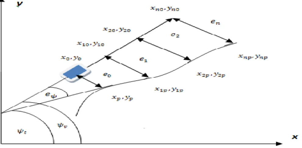
This preview distance is always on a straight line in the heading direction of the vehicle as shown in Figure 2.2. Before finding the error between the current position and the ideal position of the vehicle and the total steering angle input required for driving the vehicle on the predefined road, information about the following signals are essential to be known.
Tangent angle
Yaw angle
Present position of the vehicle
Present position of the ideal path
Ahead point position on the ideal path
All signals shown in Figure 2.2 are expressed in a fixed reference system, in which all information, i.e. angles and coordinate positions and direction, are in the same reference axis. After gathering the necessary information about different signals, three different errors are calculated. The first state feedback error named as heading error is the difference between the two angles. The second is the lateral offset distance between the ideal path position and the current position of the vehicle at current point. The last error would be calculated at the point ahead on the ideal path which is the lateral offset distance of the vehicle from the ideal path at look-ahead point as shown in Figure 2.2. One additive term named as derivative term considered in order to enhance the performance of steering controller by reducing steering wheel oscillations.
Figure 2.2: Vehicle at Generic Position
Heading error
The first state feedback error, , is the difference between the tangent angle of the ideal path and yaw angle of the vehicle at the current point.
Tangent Angle
The tangent angle, , at the point along the ideal path closest to the vehicle will allow us to find the heading error between the vehicle and the ideal path.
Yaw Angle
Yaw angle, , defined as the angle in which the vehicle is heading as shown in Figure 2.2. This heading angle used for calculating the error difference between the yaw angle and the tangent angle.
(2.2)
Position error
The second state feedback error term is the current point error as shown in Figure 2.2. It would be the lateral offset distance between the ideal path positions with the current position of vehicle. According to Figure 2.2, it could be calculated as
( )( ) ( )( ) (2.3)
Ahead-Point error
For the ahead point lateral distance error as discussed earlier, single point tracker is not worthwhile for performing the efficient path following simulation. Hence, the optical lever heading in the vehicle direction is broken down into multiple points as shown in Figure 2.2. The choice of points taken along the optical lever is user dependant. User can change the number of points on optical lever but choosing fewer points on the optical lever degrades the performance in terms of the total lateral offset distance of the current error at each point. The number of points can be decided by hit and trail according to the application, if road geometries have tight curves; larger number of points taken on the optical lever shows better results than a single or few points on the optical.
8
From the point, , the optical lever is projected straight ahead in the direction of the vehicle. For a multi-point tracker, the target point, which is being viewed on the ideal path, is subtracted from the current point on the ideal path which will enable us to get the constant step size.
√( ) ( ) (2.4)
where n is the total number of points taken on the optical lever, and is the position of target point on the ideal path whereas is the point on the ideal path closest to the vehicle.
For the first point on the optical lever, the coordinate will be calculated as:
(2.5) And for the point
(2.6) Furthermore, assuming that the distance between two points on the ideal path in Figure 2.2 is same as the distance between two points on optical lever. Taking the vehicle current position in path frame, adding step size to the x coordinate (distance along the path) and then using the PathtoWorld function to get the coordinates in the world frame as shown in Equation 2.7.
(2.7) And for the point on the ideal path
(2.8)
The PathtoWorld function is used because of the complexity involved in calculating the path coordinates in terms of mathematical equation. This PathtoWorld function will directly convert the path coordinates to world coordinates. The ‘0’ used in Equation 2.7 and Equation 2.8 is the offset distance from the ideal path which shows here that the point is directly placed on the path.
After getting the values of different points on the ideal path in world coordinates i.e. and , the error term can be calculated by using Equation 2.9 to get the lateral offset distance at the ahead point using multipoint tracker.
( )( ) ( )( ) (2.9) where extends from 1 to n, the lateral offset distances at look-ahead point will be obtained by adding up all the error terms.
Control signal
The total steering wheel input should be obtained by adding the three errors. The steering wheel input will be
∑ (2.10) where are the gains associated with different errors terms. The gains are adjusted heuristically via hits and trials for effective path following and no specific formal approach is followed for gain tuning.
Methodology of Steering Controller during Non-Linear Region
The strategy discussed in section 2.3.1 can be applied directly when the vehicle is being operated in the linear region where tyre saturation forces does not exist and vehicle is moving on the path in stable conditions. However, when road geometry has tight curves and vehicle is operating at its limits or beyond its limits, Equation 2.12 does not hold any longer during non-linear region [2].
The vehicle shows non-linear behaviour when performing at or above its maximum longitudinal and lateral limits during curves because of tyre saturation forces. For the non-linear region, saturation functions introduced at different points in order to prevent the vehicle from becoming unstable. When the vehicle operates at its limit regarding its velocity profile during cornering, control inputs in terms of steering angle would grow a great deal and the Equation 2.13 would give unsatisfactory results. Saturation functions i.e. limiters used to restrict the steering angle in specified limits in order to keep the tyre forces as close as possible which results in maximizing the control efforts [2]. This restricts the steering wheel to turn not more than the predefined limits during a manoeuvre and will eventually return the vehicle to its original path. The saturation functions used to limit and prevent different behaviours of the vehicles as described below.
There are different reasons why a vehicle becomes unstable. One reason is that its front tyres saturate first, a response known as understeer. When a vehicle understeers while performing at its limits regarding lateral acceleration, it follows a wider path than intended.
In this case, the term gives very small contribution to the total steer angle output compared to the other error terms; lateral offset distances at the current point as well as the look-ahead point. The saturation function are deployed on the other two error terms to restrict such response and to prevent the front tyre to operate far from the ideal path while maximizing the lateral controls forces to return the driver to its ideal path.
On the other hand, if the rear wheels of the vehicle saturates first, the response shown by the vehicle would be oversteer in which the major contribution in the steering wheel comes from the heading error . In this condition, the steer angle input required might be much larger than in the previous case and saturation function should be used to restrict the front wheel from steering more than the physical capacity of vehicle. A saturation function inserted on the steering angle to ensure that the steering wheel output is not larger than the predefined limits, which will restrict the wheel to rotate not more than the actual physical limits.
2.3.2 Multi-point tracker with understeer gradient
The strategy suggested by Chatzikomis et al. [3], basically use the strategy of Sharp et al. [2] for calculating the different errors by using the PD controller. Change in yaw error was used for reducing the oscillatory behaviour of vehicle during emergency manoeuvres like the lane change test as discussed in [3]. They calculate the steer angle input by using
10
(2.11)
where , and are the gains adjusted for the yaw angle, change in yaw angle and lateral offset distance respectively.
They also take the understeer and oversteer characteristics of the vehicle into account for gain scheduling [3]. They argue that generally steering angle response by the driver depends upon the velocity of the vehicle. A driver reduces the amount of steering angle when the speed of the vehicle increases. They use the ratio yaw rate by steering angle response for adjusting the steering wheel gain . The yaw rate by steering angle response was calculated by using equations for 2 degrees of freedom:
(2.12)
where V is the longitudinal velocity, l is the wheelbase length of the vehicle and the stability factor K is defined as
(2.13)
Here m is the mass of the vehicle, a and b are the distances of the front and rear axle from the centre of gravity respectively, and C1 and C2 are the cornering stiffness of the front and rear tyres.
The final steer output will be thus
(2.14)
2.3.3 Steering Controller using LQR and PID
The approach by Li et al. [4] following the linear quadratic optimal control theory in combination with the linear optimal preview time control theory has been reviewed. They use the well-known preview driver model proposed by Macadam [5].
The vehicle model used is
{ ̇ (2.15) The lateral displacement, yaw angle, lateral velocity component and yaw rate are states of the vehicle model, steering angle as control inputs for steering control and yaw rate by calculating the front and rear tyre side slip angles. The matrix A, B and C as used in [4] are used to calculate the different control variables.
The author further follows the PID controller by using methodology mention in [2] for the implementation of steering controller in which the main error used is the heading angle error. They take into account the tangent angle and heading angle of the vehicle at look-ahead point. The steer angle input is obtained by using
where is one steering angle input required for steering wheel to rotate, is tangent angle of path and is the yaw angle of vehicle at look-ahead point. Steering angle gain is adjusted by using the understeer gradient
.
(2.17)
Where l is the wheel base length, is the longitudinal velocity of vehicle, K is the stability factor, is the road coefficient and is the maximum limit with which steering wheel could be rotated.
{ | |
| | (2.18)
{ | |
| | (2.19)
Using the optimal preview control driver discussed in [4],steer input is calculated and the second steer input obtained from predicted yaw error found in Equation 2.14 are used in combination to find the total steer angle input.
(2.20)
12
Chapter 3 Methodology
The basic tools involved in development of steering controller design are Vehicle Dynamics Library; a library for vehicle simulation based on the Modelica language and Modelica standard library.
3.1 Dymola
Dymola, Dynamic Modelling Laboratory is a complete tool for modelling and simulation of integrated and complex systems for use within automotive, aerospace, robotics, process and other applications. The unique multi engineering capabilities of Dymola presents new and revolutionary solutions for modelling and simulation, as it is possible to simulate the dynamic behaviour and complex interactions between systems of many engineering fields [7]. The other useful information about Dymola can be found in [8]. The following libraries have been used while implementing the racing driver model in Dymola.
3.1.1 Modelica standard library 3.2
Package Modelica is a standardized and free package that is developed together with the Modelica language from the Modelica association [9]. This library is also called Modelica standard library. Modelica is an object oriented language developed for modelling of large and complex physical systems. It is developed for multiple domains modelling e.g. for modelling of mechatronic systems within automotive, aerospace and robotics applications. 3.1.2 Vehicle Dynamics Library
The Vehicle Dynamics Library is used to analyse the mechanical and control design of automotive chassis. The core objective is to analyse the handling behaviour of the vehicle under consideration; models are designed in a way that is similar to the structure of real vehicle assemblies [1]. The experiment shown in Figure 3.1 is from VDL, but was modified and extended for new steering controller.
Road Builder
Road builder functions used to generate various standard manoeuvres and road types. All road builder functions generate a set of tables then processed to generate the information needed for the tabular road. 2D road geometries having J turn, the extended chicane path and the closing curve path considered for testing and analysing the performance of existing and the modified steering controller.
Path velocity is not set as the vehicle is controlled from the velocity profile in the new implementation of racing driver model. Velocity along the ideal path is being controlled by the longitudinal tracker with which vehicle will be able to traverse through the path at maximum speed.
Block
Block package declared inside the ground package contains different components, which used to transform one frame coordinates into other frame coordinates/directions.
Frame
It consists of an orientation (base) and translation. The fixed reference orientation is known as the world frame, while all other local coordinate systems e.g. vehicle frame, path frame etc described with an origin and orientation expressed in world frame. The components used from block package for current steering controller implementation to resolve one frame into another are as follow.
Along Path to World Position
Along path to world position component used to resolve the path position into the world frame. Position along path is named as rV_P_x, where rV refers to vehicle position, P stands for path frame and x stands for x component along path. Using the x component in the path frame as an input to this block will convert the x component along the path to a position resolved in the world frame named as r_0[3].
View Point
This component transforms a position from world frame into driver frame r[3]. World to Ground Info
This block outputs the ground information at the position in the world frame. Input position in the world frame was resolved into ground surface x, y and z directions where the x direction along the ground surface was the tangent angle of the ideal path.
Atmosphere
The atmosphere package was defined within the VDL library for using the atmospheric effects e.g. density, atmospheric pressure etc. This component used to insert the effect of disturbances in system such as side wind during the path following, which would be helpful to analyse the performance of steering controller.
Vehicle
The vehicle model used from VDL is formula SAE chassis with double wishbone suspension having 6 degree of freedom. Steering controller was designed for FSAE and is used on different road geometries for testing and analyzing its performance. The current vehicle
14
having a mass of 200 kg, height of point center of gravity is 0.31 m and wheel base length is 1.65 m.
Driver
Driver package from VDL is used with the non-linear vehicle model to test the handling limits of vehicle while following the path efficiently. The driver template in VDL named as lateral closed loop driver is used which mainly consist of the three components.
1. Perception 2. Planner 3. Tracker
These three components integrated with each other to perform the driver steering control task by actuating the steering wheel according to the environment which human performs in the real time scenarios.
Perception:
The perception component contains information about vehicle motion states and dashboard information as perceived by the driver and then transfers this information to the planning and tracking blocks for further decisions.
Planning
This block receives inputs from perception and tracking block. The planning block calculates the error from the ideal path and forwards it to the tracking block for further operations.
Tracker
Errors calculated in the planning block are fed into tracker block. Gain tuning is performed via hit and trail for adjusting the steering wheel in order to follow the intended path.
The strategy discussed by Sharp et al. [2] in section 2.3.1 is followed, modified and further extended for the implementation of the new steering controller. This strategy does not consider the static value for tyre cornering stiffness forces and the sideslip angles estimation as well. By developing new steer planning and steer tracking block of steering controller, it would be ensured that controller follows the path more efficiently than the existing steering controller does while the vehicle was being operated either in linear region or in the non-linear region. Moreover, the multi-point tracker enables us to improve the performance significantly and the gain tuning strategy proposed by Sharp et al. [2] would be helpful for adjusting the steering angle even at high velocities without considering the understeer gradient.
The other two papers discussed in section 2.3.2 and section 2.3.3 respectively takes into account the understeer gradient. They uses the static values for cornering stiffness of tyre forces caused by the load transfer, which makes these techniques vulnerable as the tyre forces during cornering changes dynamically and measuring cornering stiffness of tyres accurately with the help of available tools supposed to be impossible yet. The sideslip angle calculation required for the lateral tyre forces changes at every point during cornering and using static values for cornering stiffness forces will not depict the realistic response.
Chapter 4 Results
The information required before adjusting the steering wheel angle is preview distance and vehicle velocity. While previewing the road ahead, different parameters need to calculate in order to adjust the steering wheel angle.
Tangent angle of the path
Yaw angle (Vehicle’s heading direction)
Lateral offset distance from the ideal path at current point
Lateral offset distance from the ideal path at ahead point
Vehicle velocity at current point
Amount of preview time for which the steering angle has to be adjusted. 4.1Implementationin Vehicle Dynamics Library
The steering controller implemented in VDL by using steer planning and steer tracking block. The new steering controller strategy for racing driver model is shown in Figure 4.1.
Figure 4.1: Steer Planning and Steer Tracking Block © Modelon AB
Implementation as well as integration of steer planning and steer tracking components in order to find the steer angle input required during the path following is discussed below. 4.1.1 Perception
The perception component shown in Figure 4.1 gathers information about vehicle motion states and dashboard information as perceived by the driver and transfers this information to planning and tracking blocks. The following information used from the perception block. The following information used from the perception block.
16
Global position of the vehicle in world frame.
Vehicle x direction resolved in world frame
Vehicle lateral offset from ideal path in the path frame x and y direction.
Yaw rate of vehicle around vehicle’s frame z axis
Vehicle Velocity 4.1.2 Steer Planning
Steer planning calculates all the errors and forwards it to the tracking block, perceived information from the perception named as percepts_in and the preview time information from the tracking block are fed into the steer planning for further processing as shown in Figure 4.2.
Figure 4.2: Steer Planning
After all the calculation performed inside sub-block in ahead point steer position, steer planning block has three error outputs which are connected with the steer tracking block.
Ahead Point Steer Position
In ahead point steer position block, the preview distance is calculated as
(4.1)
where preview time connected from the steer planning block and the vehicle velocity extracted from percepts_in component as shown below in Figure 4.3. The distance S calculated above then added with the vehicle position projected onto the ideal path, rV_P_x, to get the preview point ahead on the ideal path.
The preview point position calculated above in the path frame and the current position of the vehicle on the ideal path then forwarded to the components along path to world position, path point visualization and along path to world position1 as shown in Figure 4.3. The component along path to world position will output the path point position resolved into the world frame. Both along path to world position components connected with the tracker modified block.
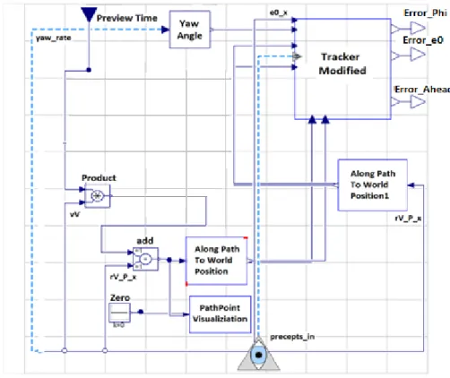
Figure 4.3: Ahead Point Steer Position
The calculated preview point on the path also fed into the path point visualization block. Path point visualization component enables to visualize the input point in the animation during simulation.
The yaw rate from percepts_in is fetched inside the yaw angle block where it is passed through an integrator to get yaw angle of vehicle at current point and forwarded to the tracker modified block. The current vehicle x direction in world frame, e0_x, from percepts_in is also connected with the tracker modified block,
Tracker Modified
Error calculations performed inside the tracker modified block. The three different errors discussed in the section 2.3calculated in this block as shown in Figure 4.4.
Error_Phi:
The purpose of this block is to implement Equation 2.2. Current position on the ideal path, rV_P_x, and the vehicle x direction in world frame, e0_x, from the perception block were fetched inside this block for calculating the difference between the tangent angle of the path and the yaw angle of the vehicle.
Tangent angle is calculated by using the vehicle closest position from ideal path, rV_P_x, it is first resolved in the world frame and extracted the vector representing the x direction, eG_0_x[3], of ideal path as shown in Figure 4.5.
18
Figure 4.4: Tracker Modified
The vehicle x direction, e0_x, is used to represents the heading direction (yaw angle) of the vehicle expressed as a vector resolved in world frame.
Figure 4.5: Error_Phi
Planar Rotation Angle
Planar rotation angle is a built-in Modelica function placed in the library named as Mechanics.Multibody.Frames. This function returns the angle of a planar rotation, given the rotation axis “e”, rotating frame 1 into frame 2 provided frame 1 is not parallel to e.
After getting the two vectors eG_0_x[3] from world to ground info and the vehicle x directione0_x[3]into the world frame from perception block, they are input to the planar rotation angle function. This will yield the heading error difference between the tangent angle of ideal path and vehicle heading direction.
Error
This error represents the offset distance of the vehicle from the ideal path at current position. The schematic of the error shown in the Figure 4.6, the vehicle position in the world frame here named as rV_0x and rV-0y for its x and y components. The x and y components of rV_P_x is here named as r_0x and r_0y respectively. This position and yaw angle were fetched inside the block error as an input. The lateral offset distance as mentioned in Equation (2.3) can be summarized as
(4.2)
Figure 4.6: Error e0
This error at current point can be calculated in a rather simple way by using the VDL built in tools shown in Figure 4.7,error represent the lateral offset distance of the vehicle from the ideal path at current point.It is implemented by using the following components for calculating the error at current point.
Current position on the ideal path; rV_P_x, was taken from the percepts_in component and connected with the path to world position component which resolves the current position on the ideal path in world frame. After resolving the current point on the ideal path into world frame, the viewpoint component is used which will transform the world frame component into driver frame.
20
Using built-in function for calculating the lateral offset instead of using Equation 4.2 gives better results numerically. The main reason behind this is as Equation 4.2 uses mathematical operation as well as the use of sine and cosine functions, which degrades the output in terms of rounding and precision.
Error Ahead
The variables required to implement Equation (2.7) shown in Figure 4.8. The global position of the vehicle in world frame, rV0_x and rV0_y, from the percepts_in connected with the optical lever block to calculate the ahead-point error. The yaw angle along with the current point and the preview point on the ideal path resolved in the world frame as shown in the Figure 4.9 connected with the optical lever block. The total lateral offset distance at the point being previewed calculated by breaking down the look-ahead point into multiple points as shown in Figure 2.2; in the present case, 10 points are being used. Constant step size obtained by using the formula for calculating the distance; see Equation 2.4, between two points. This step size is added with current vehicle position and used in Equation (2.7) to get the lateral offset distance at multiple points. Implementation of the optical lever in Modelica code using multiple points can be seen in Appendix A.
Figure 4.8: Error_Ahead-Point
After calculating these three errors, they are forwarded to the steer tracker block. 4.1.3 Steer Tracker
Steer tracker block mainly performs the gain tuning and outputs the steer angle information to steer robot after adjusting the different error gains. Steer tracker takes the vehicle velocity from perception as an input which is connected with the preview time table. Preview time with respect to vehicle velocity is extracted by performing linear interpolation. This preview time connected with the steer planning block, which uses this preview time information to get the preview distance. The other three inputs as shown in Figure 4.9 was the three errors, which were calculated in the steer planning block, these error were passed to the gain tuning block
Figure 4.9: Steer Tracker
Gain Tuning
The gain tuning block introduces the errors gain as shown in the Figure 4.10. The gain tuning was performed via hit and trial; no formal approach followed for adjusting the steering wheel gain as discussed in [3, 4] is followed. Gains adjusted would be different for different vehicle models, but once they are calculated, value could be reused for effective path following.
Derivative Term
When vehicle follows the path having tight curves, the rate of change of the heading angle error was also taken into account for reducing the high oscillations in steering wheel angle. Approximate derivative was used to perform the desire task, which will helps in smoothening the transient response as well as reducing the noise affects at the same time in steering wheel output. The approximate derivative of first order system calculated as
(4.3)
where T is the time constant, is derivative gain, is derivative output and is the heading direction of vehicle. Derivative output was combined with the other three error terms for calculating the steering wheel angle as shown in Figure 4.10.
Gain Value 5 40 0.1 0.8 T 0.01 Saturation_Intermediate 2 Saturation_Total 2
Table 4.1: Gain Values for FSAE
Gain values used for FSAE vehicle are shown in Table 4.1. Gain values used for heading angle error and look-ahead point should not be high, as it would bring the high oscillations in
22
steering wheel angle. It would be helpful in reducing the lateral offset distance from the intended path if high gain values for lateral error at current point though using very high gain value could bring oscillations in heading angle and can lead to erroneous. The derivative term; used to slower the transient response in heading angle error is helpful in reducing the oscillatory behaviour but care should be adopted in adjusting its gain. Saturation applied on the Error_Phi and on lateral error gains i.e. Error_ and Error_Optical, which restricts the error value not more than the limits defined inside the saturation block. Value of saturation functions are set in a way to prevent the rotation of steering wheel not more than the predefined limits i.e. 360˚ until the vehicle eventually returns to its original path. After adding all the gain values as shown in Figure 4.10, the steer output connector is connected with the steer robot component that will eventually turn the steering wheel to follow the path effectively.
Figure 4.10 Gain Tuning Block 4.1.4 Steer Robot
The input connector phi_ref in steer robot is connected with the str_cmd connector coming from the steer tracker block. It will eventually send the required steering control signal to the steering wheel.
4.2 Comparison of existing and new steering controller
The existing and the modified steering controller for the closed loop lateral driver model simulated on three road geometries having different curve structure. The three different road geometries are the J-turn, extended chicane and the closing curve. Total width of the road is 10 m where the ideal path is set at centreline of the road. The basic key parameter for analysing the performance of both controllers on these different paths is the lateral offset distance i.e. the total error from the ideal path at current point during the simulation. Steering wheel angle and steering wheel torque also considered for analysing and comparing the performance of both controllers. The preview distance of 10 m at velocity of 10 m/s is used for both steering controllers to make comparison with each other. Above mentioned signals for analysing steering controller are taken against distance along path instead of time which will be helpful in understanding the different results at different points on the path.
4.2.1 Path Following during J turn
The existing and the modified steering controller simulated and tested on the J turn. Length of J-turn was 300 m where the curve with radius of 50 m starts at 100 m on the ideal path and ends at 300 m as shown in Figure 4.11.
Figure 4.11: J-Turn © Modelon AB
With existing steering controller in VDL
Results of existing steering controller on the J-turn are shown and discussed below.
Steering Wheel Angle
24
Figure 4.12: Steering Angle during J-Turn (Existing Controller)
The curve on the ideal path was starting from 100 m but steering input required to turn the steering wheel along the path starts around 90 m that results in corner cutting due to which, vehicle turns before the curve starts. Furthermore, the existing steering controller exhibits constant oscillatory behaviour throughout the curve with amplitude in between to during the curve.
Steering Wheel Torque
The steering torque input required to rotate the steering wheel shown in Figure 4.13. As the steering angle input changes at every moment while following the intended path as shown in Figure 4.12, force required to turn the steering wheel also shows the oscillatory behaviour.
Figure 4.13: Steering Torque during J-Turn (Existing Controller)
With modified steering controller in VDL
The results of new steering controller during J-turn are shown below.
Steering Wheel Angle
The steering angle input required for the J-turn shown in Figure 4.14. New steering controller while showing much smoother response in terms of oscillation and required a steering angle of approximately to follow the intended path.
Steering Wheel Torque
Steering torque required to turn steering wheel shown in Figure 4.15. New steering controller requires a small amount of force during the J-turn.
Figure 4.15: Steering Torque during J-Turn (Modified Controller)
Error from the Ideal Path with existing controller
The total lateral offset distance from the ideal path was 1 m approximately as shown in Figure 4.16. During the J-turn, curve starts at 100 m; the lateral distance from the ideal path starts around 95 m and existing steering controller cannot return the vehicle back to its intended path and traverse throughout the turn with the constant lateral offset distance.
Figure 4.16: Offset from Ideal Path during J-Turn (Existing Controller)
Error from the Ideal Path with modified controller
By using the new steering controller with the predefined velocity and distance, the lateral offset from the intended path was less than 4 mm as shown in Figure 4.17.
Figure 4.17: Offset from Ideal Path during J-Turn (Modified Controller)
Existing steering controller uses atan2 function for calculating the required steer input, atan2 calculates the tangent inverse at look-ahead point. As it can be seen in Figure 4.16, the vehicle deviates from the ideal before the curve start at point 100m and the lateral offset
26
distance does not decreases throughout the curve. Because of the atan2 function, existing controller exhibits the corner cutting due to which the vehicle while trying to follow the ideal path turns its heading direction before the curve start. This is because the preview distance was set to 10 m ahead, the driver previewing 10 m ahead calculates the tangent inverse at look-ahead point, and turns the steering wheel before that input is required actually hence resulting in corner cutting. The magnitude of error depends on the preview distance being used by driver. If larger preview distance is used, the error will be greater while on the other hand, if short preview distance is being used; it will not show the corner cutting. But using smaller preview distance does not seem realistic for looking very close in front of vehicle and also it will bring oscillations regarding the steering angle and steering torque because the time to act upon the information was too short to act which eventually degrades the performance of steering controller.
The new steering controller on the other hand using a PD controller and the information about the lateral offsets from intended path follows the J-turn perfectly. The lateral offset distance from ideal path shown in Figure 4.17 was less than 4mm while restricting the oscillations in steering wheel angle as well as in steering wheel torque, which clearly makes it better than the existing steering controller does.
4.2.2Path following during extended chicane
The performance of existing and new steering controller is simulated and analysed on the extended chicane path. The extended chicane path was 250m long where the first curve of 20m radius starts from 100.1m to 150m while the second curve of 20 m starts from 150.1m and ends at 200m as shown in the Figure 4.18.
Figure 4.18: Extended Chicane Path © Modelon AB With existing steering controller in VDL
Steering Wheel Angle
The steering wheel input required with the existing steering controller for extended chicane path shown in Figure 4.19. The constant oscillatory behaviour between 100m to 200m during the two curves is obvious.
Figure 4.19: Steering Angle during extended Chicane (Existing Controller)
Steering Wheel Torque
The steering torque required to turn the steering wheel shown in Figure 4.20. The force required to turn the steering wheel does not remains constant during the two curves and driver will have to move the steering wheel continuously during the curves.
Figure 4.20: Steering Torque during extended Chicane (Existing Controller)
Modified steering controller in VDL
The results of modified steering controller during the extended chicane path are shown below.
Steering Wheel Angle
The steering wheel angle output shown in the Figure 4.21 where after some oscillations in the start of two curves, controller adjusted a smooth steering angle of approximately during the curves.
28
Steering Wheel Torque
The steering wheel torque required to turn the vehicle shown in Figure 4.22. The new steering controller exhibits very less oscillations during the curves as compared to existing steering controller as shown in Figure 4.20. The force required rotating the steering wheel increases at point 100 m and 150 m on ideal path where the two curves start.
Figure 4.22: Steering Torque during extended Chicane (Modified Controller)
Comparison of existing and modified steering controller on the extended chicane
The lateral offset distance from the ideal path for both steering controllers were calculated for comparing the performance of both steering controller on extended chicane path. The results are displayed and discussed below.
Error from the Ideal Path with existing controller
The lateral distance with the ideal path is more than 2m with existing steering controller during the two curves as shown in Figure 4.23. Error during the first curves arises around 95m whereas the turn for the first curve starts at 100m on ideal path which results in corner cutting and the driver turns the steering wheel before the curve actually starts. The same thing happens for the second curve where the vehicle is moving 2 m away from the intended path. After the end of the second curve at 200 m, the steering controller tries to reduce the error and around 235 m where vehicle return to its ideal path.
Figure 4.23: Offset from Ideal Pathduring extended Chicane (Existing Controller)
Error from the Ideal Path with modified controller
The lateral offset from ideal path by using the new controller is shown below in Figure 4.24. The maximum lateral error during the two curves is 1 cm approximately and the controller returns on the intended path quickly after exit from second curve.
Figure 4.24: Offset from Ideal Pathduring extended Chicane (Modified Controller)
The problem with existing controller is that when it encounters the curve on the road ahead, steering angle as well as steering torque shows the continuous oscillations which doesn’t decay during the curves while on the other hand, the new steering controller comparatively shows very less oscillations during the curves.
In terms of lateral offset distance from the ideal path while having the same velocities for both steering controllers, new steering controller shows much lesser amount of error in magnitude as compared to the existing controller as shown in Figure 4.23 and Figure 4.24. 4.2.3Path following during closing curve
The existing and modified steering controllers simulated on the closing curve. The length of the closing curve path was 340 m where curve starts at 50 m on the ideal path with a radius of 100 m and end up at 340 m on the ideal path having a radius of 16.66 m as shown in Figure 4.25
30
With existing steering controller in VDL
Results of existing steering controller during the closing curve are shown below.
Steering Wheel Angle
The steering wheel angle starts to increase before 50 m on the ideal as shown in Figure 4.26 and steering angle input increases as the radius of the curve decreases from 100 m to 16.66m with increasing oscillations.
Figure 4.26: Steering Angle during the Closing Curve (Existing Controller)
Steering Wheel Torque
The steering torque input required to turn steering wheel for existing steering controller shown in Figure 4.27. As can be seen, the force required to turn the steering wheel increase as the radius of the path decreases from 100 m to 16.66 m.
Figure 4.27: Steering Torque during the Closing Curve (Existing Controller)
With modified steering controller in VDL
The modified steering controller simulated on closing curve path. Results of different signals are shown below.
Steering Wheel Angle
Steering wheel input required while using the modified steering controller shown in Figure 4.28. The controller starts the turn at 50 m on ideal path and after a little oscillation; vehicle traverses the path with a smooth increasing steering angle until the end of the path.
Figure 4.28: Steering Angle during the Closing Curve (Modified Controller)
Steering Wheel Torque
The steering torque required to rotate the steering wheel shown in Figure 4.29. The force required to turn the steering wheel increases gradually as the radius of the path decreases and showing much smoother response as compared to the existing steering controller as shown in Figure 4.27.
Figure 4.29: Steering Torque during the Closing Curve (Modified Controller)
Comparison of existing and modified steering controller on the closing curve
The lateral offset with the ideal path for the existing and modified steering controller is calculated for comparing the performance of both controllers during the closing curve. The result of lateral offset distance from the intended path for both controllers are shown below.
Error with ideal path using existing controller
The lateral distance from the intended path during the closing curve increases as the curvature of the ideal path increases during the radius of 100 m to 16.66 m. As can be seen, lateral error start before 50 m as shown in Figure 4.30 due to corner cutting where the radius of the path is 100 m, and it goes on increasing as the radius of the path decreases. The error approaches 2.8 m when the radius of intended path is 16.66 m. The existing steering controller cannot reduce the lateral error throughout the curve as shown in Figure 4.30.
32
Error with ideal path using modified controller
The lateral distance from the ideal path using modified steering controller is shown in Figure 4.31. As can be seen, the lateral error from intended path is around 1 mm when the vehicle turns the curve of 16.66 m while moving at velocity of 10m/s.
Figure 4.31: Offset from Ideal Path during the Closing Curve(Modified Controller)
The performance of the modified steering controller in terms of total lateral offset distance with intended path, smoothness of steering wheel input and steering wheel torque is far better than the existing steering controller is. The modified steering controller exhibits smaller and decaying oscillations even at very tight curves as shown in Figure 4.28 and Figure 4.29. On the other hand, oscillations in steering wheel angle and steering wheel torque of existing controller increases as the curvature of the path increases as shown in Figure 4.26 and Figure 4.27. In addition, the new steering controller does not show the corner cutting while using the same preview distance of 10 m ahead on the path.
4.2.4 Side Wind Test
This test is performed for analysing the performance of both steering controller against sudden change in system. Performance of both controllers tested by simulating on a straight road where the driver experiences side wind while travelling along the road at speed of 25 m/s with look-ahead distance of 25 m. Test is conducted on the straight road having a length of 1000m as shown in the Figure 4.32 where the side wind affects the vehicle.
Figure 4.32: Straight Path © Modelon AB
A trapezoid signal used as wind speed source for the side wind test. The amplitude of the signal, the wind speed, was set to 22 m/s. The width of the trapezoid signal was 3 s plus 1 s of rising and falling edge respectively. The start time of the trapezoid signal is at 15 s during simulation where the rising edge of trapezoid signal starts. The full strength of the signal was thus within 16s to 19s, and the falling edge of side wind ended at 21 s during the simulation. The effect of side wind affecting the vehicle during simulation is shown below.