BACHELOR THESIS WITHIN: Economics NUMBER OF CREDITS: 15 ECTS
PROGRAMME OF STUDY: International Economics AUTHORS: Simon Karlsson & Charlotta Kortered JÖNKÖPING May 2020
A panel study of house price
determinants and their importance on
house prices across Swedish regions
House price variations
in Swedish regions
i
Bachelor Thesis in Economics
Title: House price variations in Swedish regions
Authors: Simon Karlsson and Charlotta Kortered
Tutor: Lina Bjerke
Date: 2020-05-18
Key terms: Regional economics, house prices, municipalities, regions, Sweden.
Abstract
The Swedish housing market has been a vastly discussed topic over the past decades due to the sharp increase in house prices. Research in the past has discussed the Swedish real estate market along with its determinants and causes, but the regional perspective of the housing market has gained less attention. In this thesis we scrutinize the Swedish housing market and its determinants with the help of a panel data set. The Swedish municipalities have been categorized into three different regions; big city, dense and rural based on their characteristics to be able to make a comparison between similar municipalities without comparing each individual municipality. A GLS estimation is used to compare these three different regions against each other in order to draw conclusions about where certain economic variables are more or less important for determining house prices. We conclude that the researched variables do vary around the country in what significance and amplitude they have on the house price levels. Furthermore, we were able to show that monetary variables have a larger influence in big city and dense regions whilst demographical and geographical variables are more important for determining house prices in rural regions.
ii
Table of Contents
1 Introduction ... 1
2 Background ... 2
3 Litterature Review ... 5
4 Data ... 10
5 Method ... 12
6 Results ... 15
8 Discussion ... 21
9 Conclusion ... 23
References ... 24
Appendix ... 28
1
1. Introduction
In the 1990’s and the early 2000’s, there was a sharp increase in the Swedish real estate prices. This brought a lot of attention to the Swedish housing market and the increase was explained by increases in disposable income of households and lowering of interest rates. When looking at the regional level, house prices were following the overall increasing trend but since the prices started at different benchmarks, they were very uneven between regions. (Yang, Wang & Campbell, 2010). This could imply that there are reasons to be concerned about the state of the Swedish real estate market.
Many of the Swedish households’ biggest asset is their property but at the same time, their biggest debt is their housing mortgage loan which could indicate that the Swedish property owners are exposed to a lot of risk in case of a negative change in the economy (Finocchiaro, Nilsson, Nyberg & Soultanaeva, 2011). Hence, it is important to investigate and be aware of what factors, including the geographical location within a country, that could affect the value of a property to know whether an investment in a property is reasonable at the time. According to Pettinger (2019), the housing market is affected by macroeconomic factors like interest rates, real income and changes in the population. Other components that can have an effect on the price are geographical distance to good schools, nature or good communications. It can also be affected by job opportunities and the availability of housing as a lower vacancy rate will lead to higher prices.
Variables that affect fluctuations in prices of residential real estate has been broadly researched both abroad and in Sweden. However, there is a gap in the research on how these variables affect different regions in Sweden. Therefore, the purpose of this thesis is to examine what economic variables that affect house prices in different types of regions in Sweden over time. By categorizing the municipalities into regions of similar character we want to investigate where certain factors are more or less significant. This will bring a regional and geographical addition to previous studies where we hope to add valuable research to what we believe is an understudied research area.
2
2. Background
Statistics show that there are large differences in how different regions grow in Sweden. In Figure 1 it is shown that the smaller regions distant from city regions have had a smaller population and lower population change compared to the dense and city regions over the time period 2001-2018. This trend can be traced back to the 1990’s and is estimated to continue until 2040 as more people are expected to move to the bigger and more densified regions in Sweden (SOU, 2015:101).
Source: Raps. Average change in population from 2001 to 2018 in rural, dense and city municipalities in Sweden
According to the Swedish Government Inquiries (SOU 2015:101), the northern municipalities in Sweden tend to have lost a part of its population over the past decades and the same goes for the Midwest of Sweden. The regions that have seen a population increase over the same time period are primarily the city regions such as Stockholm, Gothenburg and Malmo as well as the densified regions close by. These past trends are projected to continue in the future (SOU 2015:101). Statistics Sweden (2018) have a similar migration forecast and further mention that more than half of the Swedish municipalities have seen an increased population in both their corresponding cities and rural areas. This pattern is especially noticeable in municipalities with a university-city but may also be seen in the southern parts of the country and in the bigger cities along the coastlines. The population increase in municipalities nearby larger cities are also said to be at least partially correlated to the population increase in the cities over the past years (Statistics Sweden, 2018).
3
Swedish municipalities differ in both size and characteristics where northern municipalities tend to be larger in size and southern tend to be smaller, which can be seen in Figure 2. The Swedish Growth Analysis have presented a model (based on categories developed by Eurostat and OECD) where they have divided Sweden’s municipalities into three categories:
1. municipalities with less than 20% of their population in rural areas and a total population of at least 500,000 including adjacent municipalities
2. other municipalities with less than 50% of their population in rural areas
3. municipalities with at least 50% of their population in rural areas
These categories can be used to compare municipalities that have similar characteristics as there is a regional difference in Sweden (Growth Analysis, 2019). The categories are also shown in Figure 2 where all of the municipalities are displayed with a nuance of blue depending on which category they belong to. When using these different categories, it is important to distinguish between them and understand what they represent. Big city regions are in this thesis, as stated by Growth Analysis (2019), referred to the first category which has less than 20% of their population in rural areas and a total population of at least 500,000 people including adjacent municipalities. Dense regions will represent the second category, which has less than 50% of their population in rural areas. Lastly, there are rural regions which is the third category, with at least 50% of their population in rural areas1.
Proceeding in this thesis we will use the three categories mentioned above, namely rural, dense and big city. We have categorized the municipalities this way to be able to make an overall comparison between different types of municipalities rather than studying them individually. By doing this we aim to find what variables affect house prices in similar types of municipalities.
1 We would like to clarify that previous literature that is introduced in the literature review do not follow this
4
Source: Raps.
When looking at second-hand sold homes in Sweden during the period 1981 and 1997 it can be said that several macroeconomic factors like unemployment and interest rates affects the prices of Swedish homes. However, it seems that during these years, the changes in real estate prices in Stockholm had a ripple effect throughout the country. This means that the change in prices in the Stockholm region indicates the direction of real estate prices in the whole country for the following year. An increase in Stockholm would lead to an overall increase in the whole country the next year due to a lagged effect in housing prices (Berg, 2002).
5
3. Literature Review
Wilhelmsson (2008) investigated regional house prices in Sweden to see why housing prices differ between regions as well as the estimated speed of adjustment for regional house prices. By creating a model for the price-to-income ratio with employment, disposable income, income tax, mortgage rate, vacancy rate, housing stock and interest rate as independent variables, he argues that if income rises then we would expect house prices to increase and thus keep the price-to-income ratio constant. However, Wilhelmsson (2008) concludes that there are no reasons to believe that price-to-income is constant and equal over regions due to the different market conditions in different regions. As an example, it was shown that income and employment in a region had a positive effect on house prices while mortgage rates had a negative effect on house prices. Moreover, Wilhelmsson (2008) showed further evidence that the standard deviation of the house prices along with the price-to-income ratio, increased over the investigated time period around Swedish regions. This meant that the difference between high housing-cost regions versus low housing-cost regions had increased as the price-to-income ratio rose.
Low interest rates and increasing disposable income have led to increased favorable financing possibilities in Sweden which could be directly linked to the increasing house prices. By looking at income, population, vacancy rate in the renting market, turnover rate and total dwelling stock between municipalities in Sweden, it was shown that there is a significant relationship between net-migration and regional house prices due to that population growth is said to increase housing demand. Additionally, personal income and the share of people aged 25-44 had a strong significant impact on house prices in Swedish municipalities (Yang and Turner, 2004).
Different age-cohorts have different demands for housing which will have different effects on house prices. People in the age cohort 20-44 are said to put an upward pressure on house prices. This age cohort is viewed as the demand cohort, since younger people tend to have a great demand for housing and other durables. An increase in the age cohort 45-64 however, put a significant downward pressure on house prices. This older age cohort are viewed as net-lenders since they often have high financial savings and other financial investments in their possession. Hence, the age-structure of the population will influence house prices (Berg, 1996).
6
Household wealth and debt are not evenly distributed between Swedish municipalities and the most significant house prices can be found in the bigger cities like Stockholm, Gothenburg and Malmo. Households in these regions tend to have the highest share of income, but also the highest share of household liabilities partly due to the low interest rates. A clear example of this can be seen from 1997 to 2009, where there was an increase in house prices in Sweden, and 87% of this increase could be explained by higher real disposable income and lower real mortgage rates. House prices are very sensitive to interest changes and city regions are therefore exposed to more risk in case of a change in interest rates. (Yang and Turner, 2004; Frisell and Yazdi, 2010). Furthermore, when looking at the valuation of the Swedish real estate market, Dermani, Lindé and Westin (2016) found that big city regions tend to be the regions where the ratio between house prices and disposable income is the highest and they showed that that had been the case since the mid 1990’s. Municipalities with an above average income was shown to spend a larger share of their income on housing, and the relative income difference was used to explain the different house prices across Sweden (Dermani et al, 2016). Taking the relationship between income and house prices into account, Miles (2012) wanted to describe this relationship by creating a model for the major determinants of the increased house prices relative to income in the past. His model concluded that a major determinant of the increased ratio was the evolution of population density. An increased population density would also lead to an increase in income which would in the end respond to a higher house price level. Furthermore, Miles (2012) considered space a normal good, namely that as income rises one will demand more of that good. The wealthier people get, the more value they will place upon having space around them. This would in the end drive up prices in places where one will be able to get a residence or land where land is not scarce. One of the main conclusions of this study was that as population densities rise, increasing house prices are more likely to outstrip rising incomes (Miles, 2012).
When trying to estimate housing prices, vacancies have previously been taken into consideration as more available housing will give the consumer a substitute good to choose from and this could therefore affect house prices. Empirical evidence has shown a negative relationship between the amount of vacancies and housing prices in Sweden (Wilhelmsson, 2008; Gentili & Hoekstra, 2018). There is a negative relationship between the supply of housing and house prices since it restricts how many houses that are available for sale in a certain region. Housing stock adjusts slowly to market changes compared to demand factors
7
which can make it hard to measure the effect of housing stock on a short-term basis (Wilhelmsson, 2008). However, when trying to determine factors that affect house prices it is important to include a housing stock variable as housing stock/capita has a substantial impact on house prices, especially in the long-run but also in the short-run (Abelson, Joyeux, Milunovich and Chung, 2005). Further research on the housing market has shown that the demand for housing may be influenced by the way people visualize the housing market. Investigating the state of Florida in the United States, Dusansky and Koç (2007) showed that housing could be described both as a consumption and an investment good. Their research presented empirical evidence that the demand-curve for housing could be upward sloping due to that the investment component of housing could be stronger than the consumption component of housing. Hence, for the state of Florida, an increased price of housing would result in an increased demand of housing for the investigated time period, which is contradictive to the law of supply and demand (Dusansky and Koç, 2007).
When looking at Swedish mobility and its consequences for the Swedish housing market it appears that net population loss is associated with low house price levels or high vacancy rates of flats. On the contrary, there is a strong positive correlation between net-migration into a region and the house price level in that region. Regions with a large net-loss in population will have lost people in all age-cohorts, whilst regions with a large net-migration gain mostly people of the younger age-cohorts. However, a large net-migration of middle-aged people into regions is correlated with a strong housing market and a small share of vacant flats. A coastal location is also of importance for the middle-aged as well as for elderly people. (Magnusson and Turner, 2003; Yang and Turner, 2004).
Since the 1980’s there has been an increasing trend of moving between regions in Sweden. There has also been a strong increase in commuting during the same period. Short distance commuting over municipality borders has doubled and long-distance commuting has more than doubled during this time. People are less likely to move when getting older, more likely with higher education and less likely when being married (SOU 2007:35).
By looking at previous migration patterns between Swedish regions it is possible to appreciate future moving patterns between regions with a surplus of competence, to regions with a demand for workers. This can also be reflected in the number of workers that are willing to commute to closely located regions that need workers. However, regions that have the highest
8
amount of increase in commuting (into that region) have historically not had a positive net in-migration into that region. From a socioeconomic perspective it would be preferred if workers from low vacancy regions move to labor demanding regions and when looking at predictions for the future this labor-gap will be a problem, mainly for the rural and smaller regions in Sweden (SOU, 2015).
In the Netherlands, regional house prices were modelled by dividing the country into two classes which were based on the average growth rates of housing. Class one contained rural areas close to the bigger cities whilst class two consisted of both bigger cities but also rural areas around the country. If the number of commuters increases in a country it is more likely that they will live in a class one area and travel to their work in the bigger cities (part of class two). People who move away from the cities tend to be wealthy as they can afford bigger and higher quality housing in the suburbs (class one). The quality difference in housing between the two classes’ lead to a large increase in house prices in class one areas compared to class two areas. Class one areas are more sensitive, and react faster, to changes in GDP due to that a change in income may change the decision of moving out of the city and start commuting to work (Van Dijk, Frances, Paap and Van Dijk, 2009).
The real estate and housing market are moving in long cycles and a rational way of thinking is therefore to expect ever increasing or ever decreasing real estate prices depending on the current situation. By using a lag of house prices together with real income per capita, population and age structure, supply of housing and a variable for user costs it was shown that real income was the main reason of increased housing prices between 1996 and 2011 (Hansson, Karpestam and Leonhard, 2013). Furthermore, supply of housing mainly had an effect on house prices in the bigger city regions. When looking at rising income and increasing density of housing, it was also shown that housing shortage could explain more than half of the increasing housing prices of residential houses in Sweden between 1996 and 2011 (Hansson et al, 2013)
In Spain, bigger regions like the Madrid region, and other larger regions show a different trend compared to the rest of the Spanish regions due to greater demand for real estate and investments in the capital area and similar city regions. In Madrid, this could be explained by the relatively higher GDP/capita, high population density, low unemployment levels and high spending on research and development. This indicates that house prices are co-integrated between regions with similar economical characteristics and regional proximity. Hence, five
9
city regions, including the Madrid and Canaria-region have co-integrated house prices whilst all other regions in Spain are co-integrated based on their characteristics (Larraz-Iribas and Alfaro-Navarro, 2008).
Simo-Kengne (2018) studied the correlation and dynamics between house prices, population ageing and unemployment in South Africa over the period 1995 to 2015. The findings from this study showed that an ageing population had a significant negative effect on real house prices in two of the three housing segments that were investigated. An argument for this was that an increased old-age dependency ratio implies decreased savings because of a smaller working-age group and therefore less spending on housing. An argument against this was that the higher the population growth, the less likely is the dampen effect of an increased old-age dependency ratio which is often the case for less developed countries. Regarding unemployment’s effect on house prices, the study found that real estate funding partially comes from savings from the working age population and therefore it was concluded that rising unemployment had a negative effect on house prices since it creates a decreasing demand for housing (Simo-Kengne, 2018).
10
4. Data
In this thesis we utilize a panel data structure reaching from 2000 to 2018 for 289
municipalities2 in Sweden. By doing this we aim to be able to analyse regional price changes
and variations over time. Data is obtained from SCB (Statistics Sweden), Swedbank and Raps (Growth Analysis). A correlation matrix for rural (Table 6), dense (Table 7) and big city (Table 8) respectively, can be found in the appendix.
House Prices (HP)
House price is the dependent variable in this thesis. It is the average house price per year in each municipality, over 18 years. The variable is expressed in Swedish Crowns in absolute value.
Disposable Income (DI)
The independent variable disposable income is referred to as the average net income of the individuals in the municipalities in Sweden. The variable is expressed in Swedish Crowns in absolute value.
Population Density (POPDENS)
Population density is an independent variable which has been calculated as the number of persons per square kilometre (population/km²) in each municipality each year.
Net Commuting (NETCOMM)
Net commuting is an independent variable which is calculated by taking the in- minus the out-commuting each year for every municipality. The commuters considered are people who commute for work and the variable is presented in number of net commuters.
Mortgage Rate (MRATE)
This independent variable is based on the average five-year mortgage rate from Swedbank. As mortgage rates are very competitive we let Swedbank’s numbers represent the whole market over the years of interest.
2 Knivsta municipality has been excluded due to missing data points as this municipality was created in 2003. By
11
Employment Rate (EMPRATE)
This is an independent variable that represents the share of employed people of the population in each municipality each year. This variable is used as a proxy for the unemployment rate.
Ratio 20-44 (R20_44)
This independent variable represents the ratio of people aged 20-44 divided by the total population in each municipality over the time period. It is calculated to capture the demand for housing by what is considered the demand group.
Housing Stock (HSTOCK)
This independent variable represents the amount of single-family homes available in each municipality every year and should explain the supply of houses. The number of houses is in absolute value.
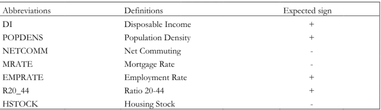
Table 1 – Expected effect of the independent variables
Abbreviations Definitions Expected sign
DI Disposable Income +
POPDENS Population Density +
NETCOMM Net Commuting -
MRATE Mortgage Rate -
EMPRATE Employment Rate +
R20_44 Ratio 20-44 +
12
5. Method
A multiple regression model is conducted for our computed panel data in order to estimate the unknown parameters. Panel data is a combination of time series and cross-sectional data and in this thesis, it involves data for 289 Swedish municipalities between 2000-2018. When estimating panel data several errors may occur because of its many implicit assumptions. This may cause the estimated coefficients and t-statistics to give misleading and inaccurate results. Errors may come from autocorrelation, heteroscedasticity and multicollinearity among other possible issues but panel data also has several advantages. Combining time series and cross-sectional data provides more informative data, more efficient data and less collinearity between the variables included compared to cross-sectional data or time series individually (Gujarati and Porter, 2009).
Three regression models will be conducted in this thesis, one for each region-type. Each of these three panel data sets are considered as a short panel where the number of cross-sections is greater than the number of time periods (Gujarati & Porter, 2009). Our selected time period is chosen to be as recent as possible to allow us to have up-to-date and relevant discussions about our results. The starting point for this research is selected to receive a balanced data set to not omitt any data points for any time period for any of the three regions.
Four general methods can be applied to analyze panel data including pooled regression, least squares dummy variable-model (LSDV), fixed effect model and random effect model. What they all have in common is that they have many implicit assumptions about their structures (Gujarati and Porter, 2009). We neglect the use of the LSDV-model due to the many cross-sections in our regression model and the problems this may cause. In the choice between a random effect model or a fixed effect model we expect a fixed effect model to be preferred over a random effect model. Likewise, in the choice between a fixed effect model and a pooled regression model we choose to proceed with a fixed effect model due to the lack of uniqueness in a pooled regression model3.
To see if our dataset fulfills the OLS assumptions of no autocorrelation between the disturbances as well as homoscedasticity in the error terms, we conduct several tests to find which model that is the most suitable for our data. From our heteroscedasticity tests we reject
13
the null hypothesis of homoscedasticity in all of our three panel data sets. We therefore break
the OLS assumption of homoscedasticity among the error terms4. From our computed tests
for autocorrelation we conclude that we have positive autocorrelation present. This problem occurs for all three panel data sets and breaks the assumption of no autocorrelation among the disturbance term (Gujarati and Porter, 2009).
Furthermore, we address the potential presence of multicollinearity in our panel data. Multicollinearity implies that there is a linear relationship between a few or all explanatory variables in an estimated regression model and its presence may lead to several errors such as insignificant t-statistics and large variances of the estimators, making it harder to do precise estimations. We utilize the variance inflation factor (VIF) to check for the level of multicollinearity across our panel data and conclude that we have a very low level of multicollinearity across our three panel data sets after recalculating all our variables with their first difference5.
In order to do empirical analysis of time series6, Gujarati and Porter (2009) argues that stationary data must be used, meaning that the variables in the time series should have a constant mean and variance over the time period. We expect to have non-stationary data in our dataset and the presence of this in an OLS estimation may result in misleading estimates of our variables. In order to test for non-stationarity in our dataset we conduct an Augmented Dickey-Fueller test and conclude that non-stationarity is present in our data set. To treat for non-stationarity, we utilize the first difference of each variable, thus making our data stationary7.
There are remedies to treat for heteroscedasticity and autocorrelation, one of them being the OLS Newey-West method. Another remedy to these situations of heteroscedasticity and autocorrelation is to use the generalized least squares method (GLS) which takes both autocorrelation and heteroscedasticity into consideration in its estimators. We have decided to proceed with this type of estimation method to adjust for our broken assumptions (Baltagi,
4 We conduct three different likelihood ratio tests of heteroscedasticity to test whether our dataset is
homoscedastic or not and conclude that all datasets show signs of heteroscedasticity.
5 Calculations for variance inflation factor (VIF) can be found in appendix.
6 Panel data is a combination of time series data and cross-sectional data; therefore, it follows the assumptions
of both data-types.
14
Kao & Na, 2011; Gujarati and Porter 2009)8. Previous research has also used this type of
estimation method for the same type of remedies, one of them being Galindo and Méndez‐ Picazo (2013). Our computed GLS estimation model looks like the following:
∆𝐻𝑃𝑖𝑡 = 𝜷𝟎+𝜷1∆𝐷𝐼𝑖𝑡 + 𝜷2 ∆𝐸𝑀𝑃𝑅𝐴𝑇𝐸𝑖𝑡+ 𝜷3∆𝐻𝑆𝑇𝑂𝐶𝐾𝑖𝑡+ 𝜷4∆𝑀𝑅𝐴𝑇𝐸𝑖𝑡
+ 𝜷5∆𝑁𝐸𝑇𝐶𝑂𝑀𝑀𝑖𝑡+ 𝜷6∆𝑃𝑂𝑃𝐷𝐸𝑁𝑆𝑖𝑡+ 𝜷7∆𝑅20 − 44𝑖𝑡+ 𝜺𝑖𝑡
(Eq. 1)
15
6. Results
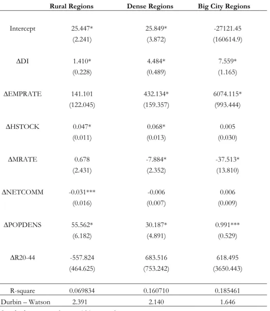
In the table below, we present the results from the three regressions that we have run using a generalized least squares estimation. We present the results for each type of region where each variable is presented with the corresponding coefficient, standard error and level of significance.
Table 2 – Panel GLS Regression Output
Rural Regions Dense Regions Big City Regions
Intercept 25.447* 25.849* -27121.45 (2.241) (3.872) (160614.9) ∆DI 1.410* 4.484* 7.559* (0.228) (0.489) (1.165) ∆EMPRATE 141.101 432.134* 6074.115* (122.045) (159.357) (993.444) ∆HSTOCK 0.047* 0.068* 0.005 (0.011) (0.013) (0.030) ∆MRATE 0.678 -7.884* -37.513* (2.431) (2.352) (13.810) ∆NETCOMM -0.031*** -0.006 0.006 (0.016) (0.007) (0.009) ∆POPDENS 55.562* 30.187* 0.991*** (6.182) (4.891) (0.529) ∆R20-44 -557.824 683.516 618.495 (464.625) (753.242) (3650.443) R-square 0.069834 0.160710 0.185461 Durbin – Watson 2.391 2.140 1.646 Standard errors are shown within parentheses.
Significant at the 1% level = *
Significant at the 5% level = **
16
Comparing the three types of municipalities gives us insight about where certain economic factors tends to affect house prices. What all the three regression outputs have in common is that they all reject the ratio of people in the age cohort 20-44 to have a significant effect on
house prices, hence contradicting the results presented by Yang and Turner, (2004). The
reasons for this could be several but one reason to why we have different results could be that there has been a change in what type of housing people in this age cohort demand in present time. Since this thesis excludes apartments and condominiums, we exclude a major part of the total real estate market and might not be able to capture the full effects.
When looking at Table 2 we can see that the relationship between house prices and housing stock is positive for dense and rural regions which goes against previous research as well as our expected result. The reasons for this result could be a lack of an explanatory variables which shows the development of the substitutable goods in the real estate market such as the market for condominiums and apartments. A positive relationship counters the research by Wilhelmsson (2008) in which he argues that there is a negative relationship between the supply of housing and house prices. Housing stock adjusts slowly to market changes and our selected time span of 18 years could therefore be too short to show the real effects regarding how the housing stock affects house prices in the long run. This is supported by Abelson et al (2005) who concludes that housing stock has a substantial impact, primarily in the long run.
Disposable income has a positive and significant relationship with house prices for all three types of regions which confirms our expectation and is in line with both the consumption
function9 and previous literature by Yang and Turner (2004). Disposable income shows the
highest estimated coefficient for big city regions which indicates that an increase in income in this type of region will lead to a significant increase in house prices within the region. Therefore, an increase in disposable income in big city regions will have a greater positive effect on house prices which is also concluded by Dermani et al, (2016). According to Yang and Turner (2004) the largest change in house prices, that are due to fluctuations in the mortgage rate, will occur in the bigger cities. This is because the highest earners, according to the study, mostly reside in the bigger cities and because of their income they can also collect a higher amount of debt than low income earners. Therefore, a large amount of people living in these big city regions have the highest share of liability and are, to a large extent exposed to a lot of risk in case of a negative change in the mortgage rate (Yang and Turner, 2004).
17
Combining previous findings with our results regarding the mortgage rate indicates that it has a bigger impact on house prices in big city regions than in other types of regions. Therefore, our results seem to support previous findings that the bigger city regions are the most sensitive to income and mortgage rate changes due to the income and wealth composition. However, we reject that mortgage rate has an effect in rural regions and can therefore not justify that a change in the mortgage rate will affect prices in these regions.
A comparison between how the employment rate in the different regions affect the house prices adds further knowledge to the above discussion about the impact of disposable income. As seen in Figure 2, the employment rate is shown to not have a significant impact on house price levels in rural regions which is not consecutive with our expectation nor in line with research by Wilhelmsson (2008). However, it seems to have a significant positive effect on house prices in dense and big city regions.
Comparing the results of dense regions with big city regions in Table 2, one can see that employment rate has a larger effect on house prices in big city regions compared to dense regions. According to Simo-Kengne (2018), unemployment will have a negative effect on consumption and house prices. Therefore, a negative change in employment rate in the big city regions will have a larger effect on house prices according to the results in Table 2. Dermani et al (2016) showed that if an unemployed person gets employed, we would expect this person to spend a larger share of their income on housing if that person lives in a big city region compared to if that person lives in a dense region. Hence, the effect on house prices in big city regions would be greater than the effect in dense regions. Furthermore, Yang and Turner (2004) argues that the bigger cities in Sweden holds the majority of the nation’s household wealth. Therefore, unemployment in a big city region could put more strain to a person’s housing affordability as compared to the rural regions due to the higher house prices in big city regions.
Furthermore, the three regions differentiate from each other when it comes to what effect net commuting has on house prices. Our regression results show that the level of net commuting does not affect the house price level in big city regions, nor in dense regions, but it appears that net commuting has a negative relationship with house prices in rural regions. This negative relationship is in line with our expectation and supports the research done by Van Dijk et al, (2009). The law of diminishing marginal product implies that an extra unit of input in to
18
a smaller capital region will bring a greater effect to production and output compared to an extra input in a larger capital region (McDowell, Bernanke, Thom, Frank & Pastine, 2012). The relatively more important role that a commuter has in rural regions as compared to dense and big city regions could be connected to the previously described law of diminishing marginal
product. Depending on the type of commuting, an increase in net-commuting in to rural regions
indicates a bigger relative impact on the housing market compared to dense or big city regions. This could be due to the smaller population and housing market in rural regions and thus, a commuter in a rural region will have a bigger marginal effect on the housing market in these regions.
Moreover, the law of diminishing marginal product may explain why our results indicate that population density has a greater effect in rural regions compared to dense and big city regions. Population density has a positive effect on house prices in each of the three region types but it appears to have the biggest effect in rural regions. Since people live less densely in rural regions, the relative effect that a person has when they move into a rural region is greater on the population growth and population density as compared to if they would move into a dense or big city region. This reasoning is also supported by Miles (2012) and in addition to his findings, we expect a person moving into a rural region to have a larger effect on the aggregate regional economy compared to if a person move into a denser region. This will bring a relatively larger effect on demand for housing in that region and could be a potential reason to why our results imply a greater effect in rural regions.
19
7. Discussion
The determinants of house prices and house price valuations have been broadly researched in the past, both domestically and internationally. Previous studies have used different types of econometrical models and have done research on different geographical levels. What this thesis contributes to the research field is a regional comparison approach for the case of Sweden where we analyse and interpret the regional house price variations and its determinants. Including economic factors that previous research has found empirically significant for determining house prices are in this thesis clustered and brought together to find their relative importance on house prices. This research does not only add a comparative approach to the regional house price determinations but it also adds further research about the housing market, its determinants and importance.
By collecting the appropriate data about the Swedish municipalities and categorizing them according to their characteristics, we were able to imply and discuss why and where certain economic factors tend to affect house price levels more or less. This adds further knowledge to the complex real estate market, but it also brings knowledge to policy makers about how certain economic factors act in relation to each other. The key contribution from this thesis is the regional approach and the comparison between the three different region types in Sweden. Furthermore, this thesis investigates the single-family house sector which means that the aggregate effect on the total real estate market is not considered. We exclude the rental sector as well as the apartment sector among others, which makes our field of study narrower considering that we capture a smaller share of the total market. The inclusion of an independent variable that is able to capture the effects of movements in the other parts of real estate market would have been a solution or suggestion to get a broader perspective. It could also show the effect between the several types of real estate in Sweden.
The primary contribution of this thesis is that it gives an insight to where and why different types of economic variables seem to be more or less relevant for determining house prices. The real estate market is complex and house prices are affected by more variables than what we are able to capture in our computed regression model. Therefore, we suggest future research on this topic to further investigate the differences in house prices across Swedish regions and why they occur.
20
In this thesis, we consider the time period 2000 to 2018 and this might imply that we are not able to capture the total effects on house prices as it takes a long time for the market to adjust (Wilhelmsson, 2008). When conducting a regression model, an increased sample size is beneficial to obtain more precise estimates (Gujarati, 2009). This could potentially be a limitation to our study as our time-span might not be sufficient in capturing the full effects of the housing market. As described earlier, panel data estimation has many implicit assumptions which may cause specification errors if they are not fulfilled. Even after correcting for the broken econometrical assumptions we found in our data, a few of our results are still not in line with previous research. Furthermore, this thesis mostly includes demand-related factors that could have an effect on the house prices and therefore, a suggestion for future studies could be to include more supply-related factors which could lead to broader and more diversified results.
The categorization of the Swedish municipalities into three different regions made it possible for us to investigate how different types of economic factors affect the Swedish municipalities differently. Another suggestion for future studies would be to scrutinize the Swedish municipalities further to receive even more specific estimates and implications.
21
8. Conclusion
The purpose of this thesis has been to analyse what economic factors that have an effect on regional house prices in Sweden from 2000 – 2018 and how their impact differs between the regions. To do this analysis we collected data from 289 Swedish municipalities and divided them into three types of regions; rural, dense and big city regions depending on their characteristics as determined by Growth Analysis (2019).
The main findings from this thesis is that there seem to be regional differences across the Swedish regions in how certain economic factors affect the house price level. We found that some of our included variables did not have a significant impact on house prices. Net-commuting has a very weak affect while the ratio of people aged 20-44 indicate to have no effect at all. However, in accordance with previous research and economic theory we found that the majority of our independent variables have a significant effect on the Swedish house prices. We find that economic variables such as disposable income and mortgage rate tend to have a bigger effect on house prices in big city regions which supports previous research (Yang and Turner, 2004). Furthermore, the results from our regression models indicate that geographical and demographical variables such as net-commuting and population density has a relatively larger impact in less dense regions, especially in rural regions. From this research, we conclude that the majority of the independent variables in this study has an effect on house prices in different region types but at different levels due to the regions’ different characteristics.
22
Reference list
Abelson, P., Joyeux, R., Milunovich, G. and Chung, D., (2005). Explaining House Prices in Australia:1970-2003*. EconomicRecord, 81(s1),pp.S96-S103.
https://doi.org/10.1111/j.1475-4932.2005.00243.x
Baltagi, B., Kao, C., & Na, S. (2011). Test of hypotheses in panel data models when the regressor and disturbances are possibly non-stationary. Asta Advances In Statistical
Analysis, 95(4), 329-350. https://doi.org/10.1007/s10182-011-0170-5
Berg, L., (1996:22). Age Distribution, Saving and Consumption in Sweden. Uppsala University: Nationalekonomiska institutionen. Advance online publication.
http://dx.doi.org/10.2139/ssrn.1405
Berg, L. (2002). Prices on the second-hand market for Swedish family houses: correlation, causation and determinants. European Journal Of Housing Policy, 2(1), 1-24.
https://doi.org/10.1080/14616710110120568
Dermani, E., Lindè, J., & Walentin, K. (2016). Bubblar det i svenska småhuspriser. Sveriges Riksbank.
http://archive.riksbank.se/Documents/Rapporter/POV/2016/2016_2/rap_pov_ar tikel_1_160922_sve.pdf
Dusansky, R., & Koç, Ç. (2007). The capital gains effect in the demand for housing. Journal
Of Urban Economics, 61(2), 287-298. https://doi.org/10.1016/j.jue.2006.07.008
Finocchiaro, D., Nilsson, C., Nyberg, D., & Soultanaeva, A. (2011). Hushållens skuldsättning,
bostadspriserna och makroekonomin: en genomgång av litteraturen (pp. 111 - 129). Sveriges
Riksbank. http://archive.riksbank.se/Upload/Rapporter/2011/RUTH/RUTH.pdf Frisell, L., & Yazdi, M. (2010). The price development in the Swedish housing market – a fundamental
analysis. Sveriges Riksbank.
http://archive.riksbank.se/Upload/Dokument_riksbank/Kat_publicerat/Artiklar_P V/2010/er_2010_3_frisell_yazdi.pdf
23
Galindo, M., & Méndez‐Picazo, M. (2013). Innovation, entrepreneurship and economic growth. Management Decision, 51(3), 501-514.
https://doi.org/10.1108/00251741311309625
Gentili, M., & Hoekstra, J. (2018). Houses without people and people without houses: a cultural and institutional exploration of an Italian paradox. Housing Studies, 34(3), 425-447. https://doi.org/10.1080/02673037.2018.1447093
Gujarati, D., & Porter, D. (2009). Basic econometrics (5th ed., pp.61-68; 320-329; 337;340; 440-449; 592-613; 741; 835). New York: McGraw-Hill.
Growth Analysis. Kommuntyper - stad och landsbygd. (2019). Retrieved 25 April 2020, from
https://tillvaxtverket.se/statistik/regional-utveckling/regionala-indelningar/kommuntyper.html
Hansson, B., Karpestam, P., & Leonhard, A. (2013). Drivs huspriserna av
bostadsbrist? Boverket. Retrieved from:
https://www.boverket.se/globalassets/publikationer/dokument/2013/drivs-huspriserna-av-bostadsbrist-marknadsrapport.pdf
Jakobsson, N. (2013). Attitudes toward municipal income tax rates in Sweden: Do people vote with their feet? Ejournal Of Tax Research; Sydney, 11(2), 157-175. Retrieved from http://proxy.library.ju.se/login?url=https://search.proquest.com/docview/1443490 081?accountid=11754
Larraz-Iribas, B. and Alfaro-Navarro, J., (2008). Asymmetric Behaviour of Spanish Regional House Prices. International Advances in Economic Research, 14(4), pp.407-421.
https://doi.org/10.1007/s11294-008-9166-7
Magnusson, L., & Turner, B. (2003). Countryside abandoned? Suburbanization and mobility in Sweden. European Journal Of Housing Policy, 3(1),
24
Miles, D. (2012). Population Density, House Prices and Mortgage Design. Scottish Journal Of
Political Economy, 59(5), 444-466. https://doi.org/10.1111/j.1467-9485.2012.00589.x
McDowell, M., Thom, R., Pastine, I., Frank, R., & Bernanke, B. (2012). Principles of
economics (3rd ed., pp. 506; 576-577). New York: McGraw-Hill Higher Education.
Muthama Musau, V. (2015). Modeling Panel Data: Comparison of GLS Estimation and Robust Covariance Matrix Estimation. American Journal Of Theoretical And Applied
Statistics, 4(3), 185. https://doi.org:10.11648/j.ajtas.20150403.25
Pettinger, T. (2019). Factors that affect the housing market - Economics Help. Retrieved 26 March 2020, from https://www.economicshelp.org/blog/377/housing/factors-that-affect-the-housing-market/
Simo-Kengne, B., (2018). Population aging, unemployment and house prices in South Africa. Journal of Housing and the Built Environment, 34(1), pp.153-174.
https://doi.org/10.1007/s10901-018-9624-3 SOU 2007:35. Flyttning och pendling i Sverige.
https://www.regeringen.se/contentassets/4b92473a96d544c68b9dfb4e86cbb013/so u-200735-flyttning-och-pendling-i-sverige
SOU 2015:101, Demografins Regionala Utmaningar.
https://www.regeringen.se/contentassets/15c00134b8b4439185d351b14765da2a/d emografins-regionala-utmaningar-sou-2015101
Statistics Sweden. (2018). Befolkningen ökar svagt på landsbygden. Retrieved 29 Feb. 2020, from https://www.scb.se/hitta-statistik/artiklar/2018/befolkningen-okar-svagt-pa-landsbygden
Van Dijk, B., Hans Franses, P., Paap, R., & van Dijk, D. (2009). Modeling regional house prices. Applied Economics, 43(17), 2097-2110. https://doi.org/10.1007/BF01434329
25
Wilhelmsson, M., (2008). Regional house prices. International Journal of Housing Markets and
Analysis, 1(1), pp.33-51.https://doi.org/10.1108/17538270810861148
Yang, Z., & Turner, B. (2004). The dynamics of Swedish national and regional house price movement. Urban Policy And Research, 22(1), 49-58.
https://doi.org/10.1080/0811114042000185482
Yang, Z., Wang, S. and Campbell, R., (2010). Monetary policy and regional price boom in Sweden. Journal of Policy Modeling, [online] 32(6), pp.865-879.
26
Appendix
Unit-root and Stationarity
There are different ways to turn a non-stationary time series into a stationary series, one of them being to utilize the first difference of each variable. By utilizing the first difference of every variable we receive the change between each year for each variable and it can lead to lower multicollinearity, more reliable t-statistics and a better estimated regression. A downside of using the first difference method for stationarity is that it reduces the sample size by the starting year. Non-stationarity may cause multicollinearity in the panel data. Multicollinearity itself does not ruin any of the assumptions of OLS but may bring uncertainty to the regression output (Gujarati and Porter, 2009). When testing for
stationarity with an augmented Dickey-Fueller test, we do not reject the null hypothesis and believe that we have a unit-root problem for all variables in all our three panel data sets. After applying the first difference method we run a new augmented Dickey-Fueller test and reject our null hypothesis meaning that we do not have a unit root problem
(non-stationarity). We thereby conclude that we have made our panel data stationary. Model choice
There are four general OLS methods that can be applied to analyze panel data. Pooled regression is an OLS estimation where all of the observations are pooled into one big regression. A drawback with this estimation method is that it neglects cross-sectional differences and camouflages the heterogeneity (uniqueness) in the data set. Least Squares Dummy Variable (LSDV) is another model which can be used to estimate panel data. This type of model allows for heterogeneity among the subjects in the panel by allowing each variable to have its own intercept. A downside of using the LSDV-model is that if one has many cross-sections in their regression, one will lose many degrees of freedom in their estimates. The more dummy variables that are introduced into a regression model, the more likely one is to suffer from multicollinearity in the regression. A third model that can be used is the fixed effect model which takes the uniqueness of each cross-section into account. The fourth model which can be used for panel data analysis is the Random Effect model (REM) which allows each cross-section to have its own intercept in the regression. (Gujarati and Porter 2009). We will not consider the LSDV-model in this thesis due to our many cross-sections within each regression model and that would cause us the loss of many degrees of freedom. To see whether a fixed effect model or a random effect model is preferred for our data set we reason about their corresponding model attributes. Random effect model
27
assumes that the included error terms are random drawings from a larger sample and it will give biased estimators if the individual error terms are correlated to one or several of the regressors. The fixed effect model will bring unbiased estimators no matter if that type of correlation exist or not. Based upon that we investigate almost every municipality in Sweden and expect to have at least some correlation between our many independent variables we disregard the random effect model in favor of a fixed effect model. We also consider a fixed effect model to be preferred over a pooled regression model since a pooled regression model neglects the cross-sectional differences. Hence, a pooled regression model
camouflages the heterogeneity of all cross-sections and consider them to be all alike which could be considered a strong assumption. Even though we have divided the municipalities in categories based upon their characteristics, we argue that there still are differences within each category.
Generalized Least Squares
OLS estimation assumes homoscedasticity of the error terms meaning that there is an equal variance of the error terms over the time period. Furthermore, OLS estimation assumes that there is no autocorrelation between the disturbances which means that there is no systematic pattern of the deviations (Gujarati & Porter, 2009). What the GLS method is applicable for is that it weighs the variance of each value against itself leading to that it does not give the same weight to each observation. Observations further away from the mean gets less weight and observations closer to the mean gets more weight as it is closer to the true value (Gujarati and Porter 2009). Another reason for why we chose to proceed with the GLS estimation method in this thesis is that the t-statistics in the regression can be interpreted correctly despite the presence of heteroscedasticity and potential autocorrelation in the data set. The absence of non-stationarity in time series is an assumption of OLS estimation methodology and gives us a third reason for using GLS, since the model can be estimated despite if its present (Baltagi,
28
Likelihood ratio test - Rural Municipalities
Specification: DHP C DDI DMRATE DNETCOMM DHSTOCK DR20-44 DPOPDENSE DEMPRATE
Null hypothesis: Residuals are homoskedastic
Value df Probability
Likelihood
Ratio 1116.671 130 0.0000
Likelihood ratio test - Dense Municipalities
Specification: DHP C DDI DMRATE DNETCOMM DHSTOCK DPOPDENSE DEMPRATED R20-44
Null hypothesis: Residuals are homoskedastic
Value df Probability
Likelihood
Ratio 926.2747 130 0.0000
Likelihood ratio test - Big City Municipalities
Specification: DHP C DDI DMRATE DNETCOMM DHSTOCK DPOPDENSE DEMPRATE DR20-44
Null hypothesis: Residuals are homoskedastic
Value df Probability Likelihood Ratio 293.3288 29 0.0000 Rural Regions Variables 1 2 3 4 5 6 7 8 1. ∆DI 1.00 2. ∆EMPRATE 0.26 1.00 3. ∆HP 0.12 0.07 1.00 4. ∆HSTOCK 0.03 -0.10 0.09 1.00 5. ∆MRATE 0.22 0.43 0.07 0.00 1.00 6. ∆NETCOMM -0.04 -0.02 -0.07 -0.01 -0.08 1.00 7. ∆PDENS 0.05 -0.01 0.16 0.11 0.03 -0.15 1.00 8. ∆R20-44 0.04 -0.08 0.00 -0.03 0.05 -0.04 0.11 1.00
29 Dense Regions Variables 1 2 3 4 5 6 7 8 1. ∆DI 1.00 2. ∆EMPRATE 0.30 1.00 3. ∆HP 0.30 0.11 1.00 4. ∆HSTOCK 0.08 -0.02 0.17 1.00 5. ∆MRATE 0.23 0.46 0.06 0.01 1.00 6. ∆NETCOMM 0.00 -0.01 -0.00 -0.00 -0.02 1.00 7. ∆PDENS 0.08 0.01 0.23 0.18 0.06 -0.04 1.00 8. ∆R20-44 0.01 -0.08 -0.01 -0.05 0.03 0.01 0.05 1.00
Big City Regions
Variables 1 2 3 4 5 6 7 8 1. ∆DI 1.00 2. ∆EMPRATE 0.25 1.00 3. ∆HP 0.30 0.27 1.00 4. ∆HSTOCK -0.01 0.02 0.01 1.00 5. ∆MRATE 0.14 0.49 0.09 0.03 1.00 6.∆NETCOMM 0.01 0.10 0.06 0.06 0.05 1.00 7. ∆PDENS 0.04 0.07 0.11 -0.04 0.04 0.13 1.00 8. ∆R20-44 0.08 0.18 0.09 0.01 0.18 -0.01 0.35 1.00
30
(Eq. 2)
i = Rural, Dense, Big City VIF Rural R² = 0.069834 gives, 1.08 Dense R² = 0.160710 gives, 1.19 Big City R² = 0.185461 gives, 1.23
According to Gujarati and Porter (2009), the rule of thumb states that a variance inflation factor (VIF) above ten is an indication of high collinearity in the regression model. The larger the value of VIF, the more troublesome is the multicollinearity in the regression. With our computed VIF of around 1.15, we expect to have low collinearity among the variables in our regression models.
Consumption function:
The consumption function shows the relation between consumption and disposable income and is written like the following:
𝐶 = 𝐶₀ + 𝑐(𝑌 − 𝑇) (Eq. 3)
This function shows that as income rises, so will consumption. If income rises 1 unit, then the consumption function tells that consumption will rise by an amount equal to c. (0< c >1) (McDowell et al, 2012)
𝑉𝐼𝐹 = 1 1 − 𝑅𝑖2