Robo-advisors on the Swedish Market:
From a Portfolio Management Perspective
MASTER THESIS WITHIN: Finance NUMBER OF CREDITS: 30
PROGRAMME OF STUDY: Civilekonom AUTHOR: Axel Berg
Sebastian Mhanga JÖNKÖPING: May 2019
1
Master Thesis in Business Administration
Title: Robo-advisors on the Swedish Market: From a Portfolio Management Perspective. Authors: Axel Berg and Sebastian Mhanga
Tutor:
Date: 2019-05-20
Key terms; Robo-advisor, portfolio management, replicate portfolio, portfolio performance, backtest, mean-variance optimisation
Abstract
Robo-advisory is a new category in portfolio management and the investment management industry. Few studies have been done on how robo-advisors’ perform in the long run. The purpose of this research is to replicate and backtest the Swedish robo-advisors’ from 2010 to 2019 and analyse their performance. Data is collected from several assets that represent the actual robo-advisors’ underlying assets. The collected data is tested through a correlation test to ensure that it accurately represents the real robo-advisors’ portfolios and performance. The portfolios’ are recreated and then backtested through the use of the online software Portfolio Visualiser. The robo-advisors’ portfolios apply mean-variance optimisation and the Black-Litterman model to allocate the assets. The research successfully replicates the robo-advisors’ portfolios and finds that one robo-advisor, Lysa, outperforms the alternatives in most risk settings and continuously delivers one of the highest risk-adjusted returns. The main contributing factor to differences in performance is found to be the proportion of stocks and bonds in the portfolios.
2
Acknowledgement
We would like to express our gratitude to our teachers at Jönköping University, our friends and our families who have all patiently helped is through this process. We want to express an extra thanks to the students that have helped us during the seminars and guided us in the right direction, and Caroline
Mhanga who has taken the time to proof read our thesis at several occasions.
3
Table of Content
1. Introduction 6
2. Background 7
2.1 The Financial System and Investment Management Industry 7
2.2 Robo-advisors 8
2.3 Problem Definition and Research Question 9
3. Literature Review 11
3.1 Market Efficiency 11
3.2 Portfolio Management and Robo-advisors 12
3.2.1 Passive Management 13
3.2.2 Active Management 13
3.3 Modern Portfolio Theory and Mean-Variance Optimization 14
3.3.1 Efficient Frontier 15
3.3.2 Capital Asset Pricing Model 16
3.3.3 Sharpe Ratio and Sortino Ratio 17
3.3.4 Black-Litterman model 18
3.4 Limitations and Critics of Mean-Variance Optimisation 19
3.4.1 Estimation Error 19
3.4.2 Time Horizon 21
3.5 Home Bias 21
3.6 Empirical Evidence and Previous Research 21
3.7 Robo-advisors’ Theoretical Framework 25
3.7.1 Avanza Auto 25
3.7.2 Lysa 27
3.7.3 Nordnet Robosave 27
3.7.4 Opti 28
4
4.1 Data Collection 29
4.2 Recreating Robo-advisors’ Asset Allocations 29
4.3 Asset Correlation 33
4.4 Benchmarks 34
4.5 Backtesting 34
4.6 Efficient Frontier 35
4.7 Estimating Net Returns 36
4:8 Limitations 37
5. Results and Analysis 38
5.1 Asset Correlation 38
5.1 Backtesting Robo-advisor Gross Returns 40
5.1.1 Aggressive Portfolio 40
5.1.2 Moderate Portfolio 43
5.1.3 Conservative Portfolio 45
5.1.4 Overall Analysis on Robo-advisors’ Performance 47
5.2 Efficient Frontier 48
5.3 Net Returns 50
6. Conclusion 53
7. Discussion 54
8. References 57
8.2 Funds, Bonds and ETFs 66
Appendices 72
Appendix A – Correlation 72
Appendix B – Portfolio weights and expense ratios 74
5
Figures
Figure 3:1, The efficient frontier.. ... 16
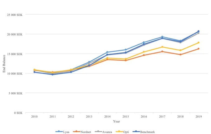
Figure 5:2, Simulated portfolio growth for an aggressive investor. ... 40
Figure 5:3, Annual return chart for robo-advisors’ aggressive portfolios. ... 42
Figure 5:4, Simulated portfolio growth for a moderate investor ... 44
Figure 5:5, Annual return chart for robo-advisors’ moderate portfolios ... 45
Figure 6:5, Simulated portfolio growth for a conservative investor ... 46
Figure 5:7, Annual return chart for robo-advisors’ conservative portfolios ... 47
Figure 5:8, Efficient Frontier between the period 2010 and 2019. ... 49
Figure 5:9, Net returns graph. ... 51
Tables
Table 4:1, Robo-advisors’ recommended portfolios for a moderate investor. ... 30Table 4:2, Proposed allocation for a moderate investor, equity quota. ... 31
Table 4:3, Proposed allocation for a moderate investor, non-equity quota. ... 32
Table 4:4, Proposed allocation for a moderate investor, all asset classes ... 33
Table 4:5, Equity to non-equity ratio used in benchmark construction. ... 34
6
1. Introduction
In the last decade robo-advisory platforms have emerged as a new financial technology (fintech) with the long-term goal to manage clients’ wealth and disintermediate the traditional investment managers (Tokic, 2018). This new approach in managing wealth and investment decisions has gained a lot of traction in terms of well-established players in the Asia-Asia-Pacific market, the U.S. market and the European market (Sironi, 2016). The largest market in terms of advisors and asset under management (AuM) is the U.S. market (Statista, 2019). The first robo-advisors in the U.S. appeared in 2006 (Mint, 2019) and several more have entered the market since. Towards 2013 the robo-advisory firms took a giant leap in becoming the top disruptive innovation in the financial market (Sironi, 2016). Robo-advisors have risen in popularity due to their user friendliness, and also due to exogenous factors such as; stricter financial regulations to protect investors like the Market in Financial Instruments Directive (MiFID II), macroeconomic factors and strong growth in U.S. stocks and the rapid increase in the number of smartphones making robo-advisors more accessible to the general public (Sironi, 2016).
The benefits of robo-advisors are their user friendliness and they generally require less capital for the initial investment in comparison to what is required by traditional investment managers (Levine & Mackey, 2017). The lower capital requirement opens up the market for the low- and medium income population as well as the HENRYs (High Earners, Not Rich Yet). Robo-advisors are positioned for exponential growth in the future as the world’s middle class and the number of high earners increase (European Banking Authority, 2019; Pezzini, 2012).
Previous research on robo-advisory has mainly covered the development of the technology and the integration with financial systems and institutions. However, research on robo-advisors’ performance is limited. This research investigates the long-term performance of Swedish robo-advisors to determine if they are a viable option for investors in the future.
7
2. Background
To understand the effect robo-advisors have had on the financial market and to determine whether they are a viable option, it is first important to understand the basics of the financial system and the evolution of robo-advisors. The following section will first look at the foundations of the financial market followed by a brief history of robo-advisors.
2.1 The Financial System and Investment Management Industry
The financial system and the investment management industry is built on financial markets and financial intermediaries which help investors transfer financial assets, real assets and financial risk in different forms. The transfer takes place when an individual or entity trades or exchanges an asset or financial contract for another (McMillan, Pinto, Pirie, Van de Venter & Kochard, 2011).
McMillan et al (2011) presents the financial system and its main purposes as follows:
1. Save - Move money from present to future with an expected rate of return given the bearing risk.
2. Borrow - Borrow money for present spending with money that the borrower does not have.
3. Raise equity - Raise money for projects by issuing ownership to investors.
4. Manage risk - Allows investors to trade assets or contracts that are correlated (or inversely correlated) with the bearing risk.
5. Exchange assets or contracts - Trade one asset for another, one currency for another or assets for money. Either for present delivery (spot market) or for future delivery (futures).
6. Trade on information - Make a profit based on information that allows investors to predict the future price.
The investment management industry is generally divided into three main branches within the supply- and demand chain; Primary/secondary issuers, intermediaries, such as investment banks, and the investors. Issuers can be equity- or debt-based offering claims such as bonds, stocks or other securities that, with the help from intermediaries, allow the issuer to fulfil their
8
financial needs or meet their requirements in risk management (Sironi, 2016). The investor can be either institutional such as government or corporation, or an individual investor i.e. taxable investor. The intermediary’s function in this industry is to transform cash flow and risk from one form to another and making a profit by linking offer (supply)-side with the demand-side. For example, intermediaries can offer investors advice for suitable products or portfolio solutions that can be achieved through direct or indirect investments. Intermediaries can also allow investors to trade products within organised and transparent frameworks through platforms (Sironi, 2016).
The investment management industry has evolved from the 1950’s high priced advisory environment to today's environment with industrialised low-priced advisory, particularly due to technological progress (Sironi, 2016). This progress has allowed automation of back office processes and transformation of investment decision making from conventional human advisory to algorithmic advisory based on risk-profiles. All of this has benefitted the final investor through reductions in costs and complexities in investment experiences (Sironi, 2016). Even if until recently investment management was exclusively conducted by human advisors, robo-advisory firms had already by 2015 accumulated asset under management in excess of 100 billion U.S. dollars (USD) and this is by many considered the beginning of the exponential growth that robo-advisory firms are facing (e.g. Beyer, 2017; Strzelczyk, 2017; Tergesen, 2015).
2.2 Robo-advisors
Sironi (p.25, 2016) defines robo-advisors as:
“Robo-advisors are automated investment solutions which engage individuals with digital tools featuring advanced customer experience, to guide them through a self-assessment process and shape their investment behaviour towards rudimentary goal-based decision-making, conveniently supported by portfolio rebalancing techniques using trading algorithms based on passive investments and diversification strategies.”
Robo-advisors first emerged on the market in 2006 (Mint, 2019) as simpler semi-automated versions of what is available today (Roboadvisors, 2018). The initial robots did not gain a lot of attraction partly due to the fact that they were introduced as personal finance management
9
tools rather than an investment tools (Mint, 2019; Roboadvisors, 2018). In 2008 the first modern robo-advisors emerged (Roboadvisors, 2018) and in 2010 the break into mainstream occurred when Jon Stein and Eli Broverman launched Betterment (Betterment, 2018; KPMG, 2016). As popularity for Betterment’s robo-advisor has increased so have the number of competitors. There are now several large companies in the US with billions of dollars in AuM (Betterment, 2018; Schwab, 2018; Wealthfront, 2018) as well as actors in other parts of the world. In Sweden the robo-advisors currently available to the public and under the government's guarantee for deposits are Lysa, Opti, Avanza Auto, Nordnet’s Robosave, Nordea’s Nora, Waizer, Fundler and Sigmastocks, the latter deviating from the rest by offering advice on purchasing specific stocks rather than mutual funds, indices and bonds. (Avanza a, 2018; Fundler, 2018; Lysa a, 2018; Nordea, 2018; Nordnet a, 2018; Opti a, 2018; Sigmastocks, 2018; Waizer, 2018).
Robo-advisors are growing at such a rate that they are becoming the primary tool for savings for the generation of today. There are many reasons why this shift from traditional investment to robo-advisors is occurring. The main reasons being the low costs offered and historically, despite the robo-advisors short history, strong risk-adjusted returns (Levine & Mackey, 2017; Sharpe, 1964). Robo-advisors offer unbiased (Faloon & Scherer, 2017), mathematical advice based on the individual's perceived risk-willingness (Jung, Dorner, Glaser & Morana, 2018). Robo-advisors essentially translate the individuals accepted risk-level (Jung, et al, 2018) into a low-cost portfolio with well diversified beta minimising the non-systematic risk (Markowitz, 1952).
2.3 Problem Definition and Research Question
Portfolio management has been studied since the beginning of the 1950’s when Markowitz (1952) published his research on modern portfolio theory. However, robo-advisory is a relatively new fintech that has not yet received extensive coverage in academic research. The research that has been conducted on robo-advisors is mainly regarding the development of the technology and the integration into the already established financial systems and institutions (e.g. Jung et al, 2018; Jung, Dorner, Weinhardt, & Pusmaz 2018; Xue, Zhu, Liu & Yin, 2018; Baker & Dellaert, 2018). A crucial factor in robo-advisors continuance and growth is performance. Are they worth the investment? To determine if robo-advisors are worth the investments the historical performance needs to be analysed. However, historical data is not available in compiled form due to the robo-advisors’ relatively recent emergence into the
10
Swedish market. For the average private investor compilation of such data is not possible due to the high costs associated with accessing and collecting the empirical data needed. As a result, there is a research gap allowing for further research on robo-advisors and their performance (Jobson, 2018).
To cover this research gap, the long-term performance of replicated robo-advisors is examined and compared with the results of relevant benchmarks. Due to robo-advisors still being a relatively new technology and way of investing, this research replicates and backtests Swedish robo-advisor portfolios over a nine-year period to be able to review and compare the replicated robo-advisors’ performance against relevant benchmarks. The purpose of the research is to replicate and investigate the long-run performance of the Swedish robo-advisors’ portfolios and answer the question: Can the Swedish robo-advisors’ portfolios be replicated and how do their long-run performance compare to a relevant benchmark?
11
3. Literature Review
To understand robo-advisors and their performance, it is important to understand the foundations which robo-advisors are built upon. Robo-advisory is an automated process to portfolio management, employing traditional theories and models when creating portfolios. The following section covers the literature, theories and models that robo-advisors utilise, starting with market efficiency, portfolio management and modern portfolio theory. Thereafter, limitations to the theories are highlighted followed by a review of previous research on robo-advisors.
3.1 Market Efficiency
In the 1960’s Eugene Fama introduced the Efficient market hypothesis (Fama, 1960). The hypothesis has been one of the foundations for how investors of all types, being professional investors, non-professional individuals or computers trading on algorithms, select their investments regardless of what specific investment strategy and philosophy they believe is superior. The hypothesis is a corner stone to investing as investors either believe it holds, entailing that all available information is already reflected in the stock price, or it does not. Should the investor not accept the efficient market hypothesis (EMH), the investor then believes he or she is able to find price discrepancies in stocks and capitalise on these (Bodie, Kane & Marcus, 2014). Fama’s hypothesis sprung from the work of Maurice Kendall (1953, Bodie et al, 2014) who examined the predictability of stock prices when examining stock performance over a set period of time. Kendall found that stock prices appear to be random and there is no apparent pattern and based on the data collected there was no way to predict future stock prices. (Kendall, 1953). From Kendall’s research the argument of stock prices following a “random walk” was born. Stock prices reflect the current information and any known future information is already reflected in the stock price. It is only new and unpredicted information which affects the stock price. This information will quickly be reflected in the stock price and as the stock price moves in a seemingly random pattern to the new level the random walk Kendall observed is in fact the market adjusting to new information, thus the efficient market hypothesis stated by Fama holds as the stock price reflects all currently available information (Malkiel, 2016). While Fama’s EMH has played a large role in how investors choose their stocks since its publication in the 1960’s, its relevance and accuracy has been questioned. Robert Shiller is part
12
of the opposition claiming that the EMH does not hold. Through empirical studies Shiller has come to the conclusion that “random walks” in stock prices are too random to be a reflection of the available information (Shiller, 1981). An example used by Burton (2003) that reflects how EMH stated by Fama in the 60’s does not reflect how the stock market works in an accurate way is described in Burton’s book “A random walk down wall street”. He recounts a story of a finance professor and a student. The student stumbles across a 100-dollar bill on the ground. The professor then proceeds to say, “Don’t bother picking it up, if it were real it would not be there”. This anecdote aims to explains how financial markets are efficient and that there are no free 100-dollar bills lying around for investors to pick up. As there are plenty of investors who invest with the strategy of finding misplaced stocks the EMH has later been revised stating that markets are close to efficient most of the time. The investors who aim to exploit the discrepancies in stock prices and the perceived (actual) value of the stock are a necessity for the markets to function in an efficient way as these actors bring the prices in line with the intrinsic value of the stock and the current information available (Bodie et al, 2014).
In 1980 Grossman and Stiglitz published their research “On the impossibility of informationally efficient markets”. The cost incurred by investors who seek to invest in mis-priced stocks is taken into account in the model created by Grossman and Stiglitz. They go on to illustrate how the investors willingness to pay the cost for the additional information to find the mis-priced stocks should be compensated with higher returns as investors are rational and seek the maximum returns. This goes to explain the revised and modern view on EMH where markets are mostly efficient almost all of the time. The investors who seek excess return incur costs in pursuing the information required to generate these excess returns these investments are ultimately what cause the market to act efficiently (Fama, 1970).
3.2 Portfolio Management and Robo-advisors
Investment managers can find determinants of portfolio performance in three activities that compose the process of portfolio management - Investment policy, security selection and market timing. Studies made on large U.S. pension plans shows that total return from investment policy itself is 93.6 per cent and therefor investment policy is the solely most important part in portfolio management and is often called strategic allocation (Brinson, Hood & Beebower, 1986). Investment policy, or strategic allocation, determines which asset classes and weights that should be selected to meet the investors target (Brinson et al, 1986). Given the
13
asset’s class and its weights, since each asset class is associated with its own risk and return, the investment manager needs to decide his or her risk tolerance, investment horizon and the investments risk level (Cochrane, 1999).
Robo-advisory has been around since 2006 and is a new way of portfolio management. It is basically an automated process of the previous mentioned steps; selection of investment in assets that match the client’s preferences towards risk and reward. It automates the traditional process of selecting asset classes and weights by using algorithms to place investors in different portfolios based on the investors’ risk aversion. To feed the algorithm with information the investor answers the questionnaire online about his or her risk tolerance (Moyer, 2015).
3.2.1 Passive Management
Portfolio management can be divided into two subcategories; active or passive management (Al-Aradi & Jaimungal, 2018; Sharpe, 1991). Initially, a security market is chosen, for example OMXS 30 or S&P 500. Thereafter an investor must choose whether to be active or passive. The passive investor buys and holds all the market’s underlying securities according to the weight that each security represents in the market (Jasmeen & Satyanarayana, 2012, Sharpe, 1991). If security X represents 2 per cent of the market, the passive investors portfolio will contain 2 per cent of security X. The passive investor will obtain precisely the same return as the market and incurs a low cost due to little or no research behind asset selection and the avoidance of transaction costs as a result of low trading frequency (Sharpe, 1991). The passive investor therefore believes that they have more to gain trying to reduce his or her costs rather than trying to beat the market itself. With passive management, following market representation, a wide diversification can be enjoyed which is an important contribution to robo-advisors passive management strategies.
3.2.2 Active Management
Actively managed portfolios create value to its investors in two ways; (a) the portfolio managers goal is to select portfolio securities and its allocation in a way that provides a superior return towards purchasing an index such as S&P 500 and (b) continuously revising security allocation and monitoring securities as well as market conditions. If a fund manager is successful in both these processes, he or she will be considered successful and beat the benchmark (Shukla, 2004). Active management is an expensive way to manage a portfolio and will only add value towards
14
its investors if the excess return after costs is larger than the incremental cost it adds towards its investors (Sharpe, 1991).
Sharpe (p.7, 1991) was strongly opposed to active management with support and argument for law of arithmetic. Sharpe meant that, in a mathematical way:
“If active and passive management styles are defined in a reasonable way, it must be the case that:
(a) Before costs, the return on the average actively managed dollar will equal the return on the average passively managed dollar and
(b) after costs, the return on the average actively managed dollar will be less than the return on the average passively managed dollar.”
Sharpe (1991) meant that these claims will hold for any time and that they depend on the law of addition, multiplication, subtraction and division. Sharpe goes on to say that to justify anyone who claims to be a successful active manager, the individual must conveniently have been excluded from the law of arithmetic. This conclusion made by Sharpe (1999) emphasises that active management is a zero-sum game. If there are winners, there must also be losers.
3.3 Modern Portfolio Theory and Mean-Variance Optimization
Mean-variance optimization (MVO) is the base for many modern portfolio theories and models. First published by Markowitz in 1952 it has been and still is the foundation portfolio selection. MVO is the framework for asset selection assessing expected return and covariance to determine the appropriate weight in a portfolio. Modern portfolio theory and MVO are today interchangeable describing the same theory (Kritzman, 2011; Markowitz, 1952).
Markowitz’s theory uses diversification to decrease portfolio risk by investing in several assets with low correlation. Diversification does not eliminate risk completely but works to bring the unsystematic risk to a minimum, by choosing risky assets to increase the expected return of the portfolio but diversifying by choosing assets with a low correlation to the rest of the portfolio. By creating such a portfolio, risky assets with low correlation to each other and the overall portfolio, Markowitz’s theory allows for a portfolio with high expected return but a portfolio risk lower than that of each individual firm’s risk but still keeping the portfolio’s expected
15
return the same as the weighted average expected return of the portfolio assets (Markowitz, 1952). The modern-portfolio theory is visually presented in one of the theory’s cornerstones, the Efficient frontier (EF) (Michaud, 1952). The EF is the combination of assets, i.e. a portfolio, which satisfies the condition that there are no other combinations of assets which generate a higher expected return without incurring higher risk (Markowitz, 1952). The EF will be further explained in the following heading.
The number of assets in the portfolio to reach sufficient diversification is still under dispute but it is clear that an increased amount of assets lowers portfolio risk. Evans and Archer (1968) found that as little as 10 stocks was enough for sufficient diversification while later studies have shown that a portfolio of 100 stocks has 32 per cent lower risk than a portfolio comprised of 15 stocks (Elton & Gruber, 1977). While the amount of stocks required for a diversified portfolio is under a lot of discussion Statman (1987) found that a minimum of 30 stocks is required for a diversified portfolio. There has been little research on the subject of the number of stocks in a well-diversified portfolio however Evan’s and Archer’s (1968) observations showed a linear relationship between a higher number of stocks and a lower portfolio volatility. This linear relationship is further observed by Fama and French (2010). They found that fund managers in general do not generate excess risk-adjusted returns in the long run and identifying what fund managers will generate greater returns than the market is impossible. Hickey, Lungo, Nielson and Zhang (2015) further investigate the relationship between number of stocks and the portfolio performance finding that funds with a low number of stocks have higher volatility than funds with a large number of stocks. Their findings are also supported by previous research by Newould and Poon (1996).
3.3.1 Efficient Frontier
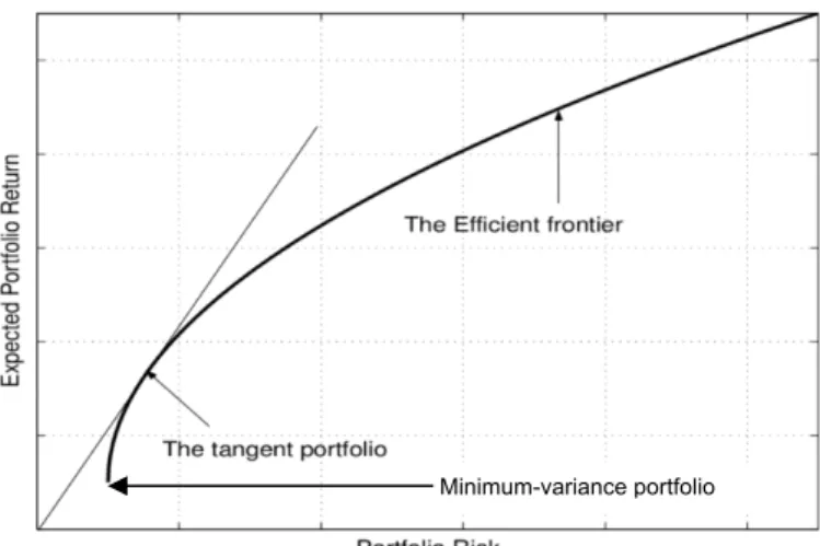
The efficient frontier graphically presents the combinations of assets which create a portfolio with a maximised expected return in regard to the inferred risk. The efficient frontiers' visual presentation can be seen in figure 3:1. Any portfolio that is below or to the right of the efficient frontier is unwanted as they do not offer a sufficient risk-return ratio with a risk to high for the expected return (Markowitz, 1952). The straight line touching the efficient frontier is the Capital Allocation Line (CAL). The point where the efficient frontier and CAL touch is the optimal portfolio for the investor maximising the expected return given the risk. This point is also called the Tangency Portfolio (Keykhaei & Jahandideh 2013; Tobin, 1958).
16
All portfolios are plotted within the efficient frontier hyperbola and as seen in figure 3:1 the tangency portfolio is located where the CAL and efficient frontier touch. The minimum-variance portfolio (Maillet, Tokpavi, & Vaucher, 2015) is located at the point on the efficient frontier where it crosses from the lower and sub-optimal portfolios to the upper part of the efficient frontier where the desired portfolios, primarily the tangency portfolio, are located or simply put, the location on the efficient frontier with the lowest standard deviation (Markowitz, 1952).
3.3.2 Capital Asset Pricing Model
The Capital asset pricing model (CAPM) was developed independently by Treynor (1961, 1962), William F. Sharpe (1964), John Lintner (1965) and Jan Mossin (1966). The model is a development of Markowitz’s modern portfolio theory and determines the return of an asset required for it to be placed in a diversified portfolio (Sharpe, 1964). In other words, CAPM is used to price securities with a certain level of risk and determining the expected return of the investment given the risk-free rate of the market and the beta of the investment.
CAPM applies four assumptions (Sharpe, 1964). 1. Investors are risk averse
2. Investors incur no transaction costs or taxes, all trades are done at competitive market prices and borrowing and lending occurs at the risk-free interest rate.
Figure 3:1, The efficient frontier. Expected return increases on the y-axis as the risk increases on the x-axis. The hyperbola represents the efficient frontier and the straight line originating from where expected return and risk is 0 is the CAL. The lowest part of the efficient frontier is the minimum-variance portfolio, portfolios below are sub-optimal (Fabozzi, Rachev & Stoyanov, 2007).
17
3. Investors are rational and invest in efficient portfolios based on the same available information.
4. Investors are homogenous in their expectations concerning volatility, return and correlations.
With these four assumptions CAPM works as a theory of equilibrium where homogenous investors identify the same efficient portfolio with the highest Sharpe ratio (Perold, 2004). As all investors price assets according to CAPM the supply and demand for risky asset must be in equilibrium. As a result, all investors will hold equal proportions of risky-assets. If all investors hold these same proportions this must be the proportion of risky assets held in the market portfolio. Thus, the efficient portfolio with the highest Sharpe ratio is the market portfolio (Perold, 2004). Treynor, Sharpe, Lintner and Mossin found the relation between the expected return of the portfolio and the expected return of the market portfolio to be:
Ε(𝑅$) = 𝑅'+ 𝛽$(𝐸(𝑅+) − 𝑅') Ε(𝑅$) = Expected return on the investment
𝑅' = Risk free rate of return 𝛽$ = Beta value
𝐸(𝑅+) = Expected market return
According to CAPM, if this formula does not hold there is a mispricing in the market and investors can outperform the market by obtaining a higher Sharpe ratio until the price is adjusted to the level where the CAPM formula holds (Perold, 2004).
3.3.3 Sharpe Ratio and Sortino Ratio
The Sharpe ratio and Sortino ratio are both measures for examining the risk-to-reward ratio of an investment. The Sharpe ratio was developed by William F. Sharpe in 1966 (Sharpe, 1966) and measures the relationship of excess return to the risk of the investment. The formula is calculated through dividing the market premium by the standard deviation (Sharpe, 1966):
S = 𝐸[𝑅 − 𝑅'] √𝑣𝑎𝑟[𝑅]
18
S=Sharpe ratio E=Expected return R= Asset return
𝑅'=Risk free rate of return
√𝑣𝑎𝑟[𝑅]= Standard deviation of the assets returns
In 1994 Sharpe published a revised version of the Sharpe ratio where the standard deviation of the asset’s return is replaced with the standard deviation of the risk premium. The revised version of the Sharp ratio is as follows (Sharpe, 1994):
S = 𝐸[𝑅 − 𝑅4] √𝑣𝑎𝑟[𝑅 − 𝑅4]
𝑅4= risk free rate of return
The Sortino ratio is a modification of the Sharpe ratio created by Frank A. Sortino and Lee N. Price (van Der Meer & Sortino 1994; Price & Sortino, 1991). As distinct from the Sharpe ratio, Sortino ratio only penalizes the negative deviations (Price & Sortino, 1991). As a result, the Sortino ratio is used to asses and compare downside risk while the Sharpe ratio is affected by both negative and positive returns that deviate from the mean. The Sortino ratio is calculated as follows (Price & Sortino, 1994):
𝑆 =𝑅6𝜎− 𝑇 9
S = Sortino ratio
𝑅6= Actual or expected return of the portfolio
T = Target return (originally MAR, Minimum Accepted Return). Often the risk-free rate
𝜎9= Downside standard deviations
3.3.4 Black-Litterman model
The Black-Litterman model (BLM) (1992) is a practical interpretation of MVO allowing for a model that is more applicable to real life investments. MVO acts under the assumption that the expected return and covariance is known and has been an important theoretical contribution to portfolio theory. In real world investments estimating an accurate expected return of assets is a strenuous task rendering MVO less viable in practice (Black & Litterman, 1992). MVO presents
19
the problem where it allocates all the capital to only a few assets creating a concentrated portfolio due to the estimation errors of the expected returns (O'Toole, 2013). The BLM offers a smoother approach more viable in practice where the investor’s beliefs are taken into account and overcomes the problem of portfolios being highly sensitive to expected returns (Black & Litterman, 1992).
3.4 Limitations and Critics of Mean-Variance Optimisation
Even though the mean-variance approach is the standard theoretical model and is widely used in portfolio management, asset allocation is the school book example for the method of choice for optimal portfolio construction, it contains some problems which makes the approach impractical to use in asset management due to its limitations. This part will cover the limitations that the traditional MVO approach has when using it with default settings.
3.4.1 Estimation Error
The first limitation to MVO is estimation error. The parameters being used in Markowitz’s modern portfolio theory are the means, correlations of security returns and the standard deviations. These parameters can be estimates in a number of ways, such as historical data, analytical models and analytical forecasts. When the investor uses historical data to estimate the parameters estimation errors are a main concern (Broadie, 1993). Estimation error, or maximization estimation error, is perhaps also the most severe limitation of the theory since the risk and return estimates are inescapable subjects for estimation errors. What estimation error contributes with is heavy over- or underweighting in certain securities which have large or small estimated returns, negative or positive correlations and large or small variances. Securities that fulfil any of these criteria are most likely subjects to have a large estimation error (Michaud, 1989). The problem and consequence with estimation error is that the measure of diverse risk that is constructed by the ”optimal” portfolio is likely to be a great underestimation of the optimal portfolios actual risk. Due to the framework’s sensitivity to these inputs, Michaud (1989) claims that MVO often does more harm to a portfolio than it does good.
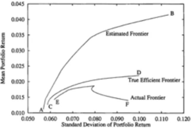
Studies show that using expected, or estimated, value rather than ”true” parameters will give estimation errors. Even if the estimation errors are relatively small can it still be a significant difference in portfolio weights amongst the portfolio investment vehicles. Broadie (1999) shows in his study the difference in outcome between the estimated frontier, true efficient
20
frontier and the actual frontier, seen in figure 3:1. The estimated frontier uses estimated parameters and the actual frontier uses the same weights as the estimated frontier but with true means and variances. The true efficient frontier and the actual frontier are unobservable due to their true and unknown parameters. The only frontier that is observable in practice and therefore appear to be the case is the estimated frontier, but the actual frontier is what really occurs due to its in fact true parameters. Due to the actual frontiers estimation errors it will always be placed far from the true efficient frontier and even more far from the estimated frontier. Smith and Winkler (2006) defines this phenomenon as “the optimizer’s curse” since actual outcomes on average are worse than the original estimates on parameters.
Figure 3:2. Mean-variance frontiers (Broadie, 1999).
Studies conducted by Best and Gauer (1991) show the impact that estimation errors have on a portfolio. In their studies they tested how sensitive an MVO portfolio was to changes. According to their findings a mean change of 11.6 per cent triggered half of the equally weighted portfolio to re-allocate into the asset that now has changed. These findings confirm the importance of precision in the data and estimates that need to be done to successfully execute MV-portfolio optimization.
To solve the problem with estimation error Broadie (1999) recommends practitioners to use historical data for estimation of the standard deviations and correlations. Broadie (1999) recommends the use of a model to estimate mean returns since these are the most complicated to estimate. Another solution comes from Swensen (2009) who suggests adding more constraints into the formula in order to avoid unreasonable or extreme weights of certain asset
21
classes. Swensen’s weight constraints span from a lower limit of five per cent to an upper limit of twenty-five to thirty per cent limit for each certain asset class weight.
3.4.2 Time Horizon
The second limitation of MVO is the time horizon in the framework. The MVO framework is based on a single-time period model and is most often used during a 1-year time period. This can be done, given that asset returns are independent of each other, so that short term (annual) periods can be used in order to characterize estimates for long term returns. This results in the problem with this is that many investors often have longer time periods for their investments. This dilemma results in investment decisions made according to the MVO being sub-optimal to the investor (Swensen, 2009).
Goetzmann and Edwards (1994) conducted a study, incorporating auto-correlation, where they simulated long-term and short-term returns of different assets and found that short-term returns lead to an incorrect conclusion of the compositions in the mean-variance portfolio as well as changes in the efficient frontier. Goetzmann and Edwards (1994) build their approach on the necessity of investors’ time-frame being defined. Markowitz’s model is not applicable since time-series behaviour is such a critical part of the estimates.
3.5 Home Bias
Home bias is a regular occurrence in portfolio management and asset selection (Perold, 2004). Some research claims that the home bias of funds is a lot higher than previously believed (Ke, Ng & Wang, 2009). Perold (2004) argues that the main reason for investors and portfolio managers exhibiting home bias is because of relative purchasing power. Investors’ income and purchasing power is correlated with the stock market of that investor’s home country, increases in the stock market will benefit the investor and market declines will affect all domestic investors and due to this investors are more inclined to be heavily invested in their home markets to not miss an increase in the domestic market.
3.6 Empirical Evidence and Previous Research
The most common strategy applied by Robo-advisors is passive portfolio management. The following section will therefore cover empirical evidence and studies that has been made on the strategy. Portfolio management is a well-established area of studies and with numerous
22
empirical studies on the market efficiency. Some studies are making strong cases of passive management and other studies commend for strategies in trading which have generated returns excess of the risk it is holding. Due to market inefficiency, strategies that are generating risk-adjusted excess return can never exclude the possibility of pricing models being erroneous regarding the model’s perspective on risk and return. This uncertainty makes any definite contradiction of the efficient market hypothesis virtually impossible (Campbell, Lo, Mackinlay & Whitelaw, 1997).
The main conclusions that can be made from Brinson et al. (1991; 1986) are that a majority of the research which has been conducted within the field of studies makes a case for actively managed funds on average being less successful in generating excess return net of their costs, meanwhile previous research which isolate the skills of portfolio managers presents which managers on average are successful in the selection assets that exceed the market performance (Berk & Van Binsbergen, 2012; Kosowski, Timmermann, Wermers & White, 2006; Ibbotson & Kaplan, 2000). Brinson et al. (1991; 1986) base this conclusion on their research where investment policy or strategic allocation stood for a greater part of the total return and also explained over 90 percentage of the total variation in the returns. The total return in a portfolio consists of the net result on the security selection, market timing and strategic allocation of asset classes.
Research on robo-advisory within the financial services industry has been made. However, this research is mainly focused on Robo-advisory as a disruptive technology and how it will act in the wealth management industry. Studies have concluded that current generation of robo-advisors main focuses are financial regulations, minimizing cost and offering simplistic wealth management to its customers (Jung et. al, 2018; Xue et. al, 2018; Baker & Dellaert, 2018; Ji, 2017) Recent studies urge the next generation of robo-advisors to elaborate on behavioural peculiarities with customers’ preferences and enable personalisation to a higher extent (Jung et. al, 2018; Xue et. al, 2018; Faloon & Scherer, 2017). Other studies that have been made on robo-advisors conclude that robo-robo-advisors are a major advance in the investment management industry. Due to automatization, investment services, which previously required highly educated and expensive personnel, will now be available to a broader market. As a result, more investors will have better portfolios and investments (Beyer, 2017; Scherer, 2017; Hougan, 2015).
23
As previously mentioned, studies on robo-advisors’ performance are scarce. A study by Bjerknes & Vukovic (2017) investigates and replicates the performance of U.S. robo-advisors as well as trying to simulate a fictitious robo-advisor and its performance on the Norwegian market. There are no studies conducted on robo-advisors performance on the Swedish market. On the following page, Table 3:1 presents some recent studies on robo-advisors.
24
Table 3:1, Previous studies on robo-advisors with summary of the results. Sorted by date.
Study Author(s) Subject Results and finding
Designing a robo-advisor for risk-averse, low budget consumers Jung, Dorner, Weinhardt & Pusmaz (2018). Robo-advisor design
Identify requirements and design principles. BlackRock Robo-Advisor 4.0: When AI replace human discretion Tokic (2018). Robo-advisor design
Case to replace human discretion with AI. Group Recommendation
based on Financial Social Network for Robo-Advisor
Xue, Zhu & Yin
(2018). Categorise users risk preference. Risk recommendation model for groups with filtering algorithms.
Robo-Advisory Jung, Dorner, Glaser & Morana (2018).
Design and outlook
Today robo-advisors target underdeveloped retail customers.
Human vulnerability and
robo-advisory Beltramini (2018). Human vulnerability Suggest an approach to machine-human interface for human vulnerability rather than machine’s performance. Humans versus ROBOTS Levine & Mackey
(2018).
Human vs Robots
Robots can easily replace humans. Human action needs to be justified with added value.
Has Your Advice Evolved with Technology?
Pandya (2018). Financial planning
Financial institutions need to engage technology into their practice.
Are Robots Good Fiduciaries? Regulating Robo-Advisors
Ji (2017). Regulations Regulations should focus on loyalty issues at to avoid conflicts of interest. Automated Advice: A Portfolio Management Perspective on Robo-Advisors Bjerknes & Vukovic (2017). Estimate robo-advisors’ performance
Replicates U.S. Robo-advisor performance and simulate fictive robo-advisor on Norwegian market. Algorithmic Portfolio
Choice: A lessons from panel survey data
Scherer (2017). Investor risk variables
Assess set of variables to be included in algorithmic portfolio advice. Robo-Advisers: What it Means to You Hougan (2015). Human vs Robots
Robots need to offer truly differentiated solutions to survive. Humans need to leverage on robo-advisors.
25
3.7 Robo-advisors’ Theoretical Framework
This research studies Lysa, Nordnet Avanza and Opti. These robo-advisors are chosen because of their available data and the transparency of their portfolio details. The robo-advisors observed in this paper all apply a systematic approach to investing and the asset selection process (Avanza b, 2019; Lysa b, 2019; Nordnet b, 2019; Opti b, 2019). The underlying assumptions and theoretical frameworks are; The EMH, Markowitz portfolio optimisation model, CAPM and risk-adjusted returns. The robots have different underlying funds as assets that have been chosen at discretion of the individual companies and their analysts. These funds all share the common feature of being low cost index funds tracking a broad index with passive management enabling the low costs (Avanza b, 2019; Lysa b, 2019; Nordnet b, 2019; Opti b, 2019). In the following section each Robo-advisors’ portfolio selection process will be studied.
3.7.1 Avanza Auto
Avanza Auto does not give the investor direct ownership in the funds invested in. Instead there are 6 pre-set portfolios offered which are recommended depending on the individual's acceptance of risk and the length of the investment. Portfolio 1-3 are for short-term investments with a time horizon of 5 years or less and portfolio 4-6 are for long-term investments with a time horizon of more than 5 year. Regardless of what portfolio is chosen by the investor there is no limit to when or how much can be withdrawn (Avanza b, 2019).
Avanza Auto utilise the practical application of Markowitz’s theory which was developed by Fisher Black and Robert Litterman (1992). The Black-Litterman approach assumes that the observable market portfolio is efficient. The optimal portfolio is achieved by combining the market portfolio and the managers belief of how the implicit weighted returns will develop over time.
Avanza Autos systematic and quantitative model is divided into 3 stages.
Stage 1 identifies the market portfolios assets, their weights and their respective equilibrium returns. Stage 2 combines the market portfolio and the given weights with the investor or portfolio managers belief of the future performance of the market portfolio and the stock market as a whole. Avanza autos model 50 per cent confidence interval that the investor or portfolio
26
managers belief of the markets future performance will prove accurate (Avanza b, 2019). Stage 3 applies a set of restrictions (see below) to avoid unrealistic purely mathematical portfolios.
• Short positions are not allowed
• The highest allowed average cost of the underlying funds is 0,15 per cent. • A minimum exposure to the Swedish market of 15 per cent.
• Investments must be in-line with Avanza funds sustainability instructions.
• Restrictions in the allocation between stocks, interests (bonds) and alternative investments.
• Restrictions to avoid assets from deviating too much from their weights in the market portfolio (with the exception from Sweden).
The portfolio allocation is spread over three different types of investments; Stocks, Interests (bonds) and alternative investments. The primary assets are stocks to increase the return and bonds for controlling and decreasing risk. Alternative investments are sometimes used as a secondary investment to increase diversification and improve the risk-reward ratio.
The asset allocation is executed with the belief of stocks yielding a greater return than that of bonds and that the Swedish market will yield greater returns than other markets. This belief combined with the greater knowledge of the Swedish market is the reason to the home bias in the portfolio composition. In addition to this Avanza identifies and acknowledges the U.S. market as one of the world’s most important markets and as a result allows for the option of increased investments in U.S. small-cap stocks. Avanza autos asset classes can be seen in the table below (Avanza b, 2019).
Rebalancing occurs primarily quarterly to keep the portfolios given weight and risk levels. If an assets weight diverges greatly from the given weight, there are measures in place to automatically rebalance the portfolio to ensure weights are in accordance with the portfolio generated by the Black-Litterman model. In addition to quarterly rebalancing of the portfolio weights the optimal allocation is re-calculated and performance is analysed annually for each of the 6 Avanza Auto portfolios (Avanza b, 2019).
27
3.7.2 Lysa
The investment process of Lysa is similar to that of Avanza Auto where the investor does not get direct ownership in the underlying funds. The investor’s portfolio is a mix of “Lysa aktier”,
aktier translating into stocks, and “Lysa räntor”, where räntor translates to interest achieved
mainly through bonds. Depending on the given risk-level and time horizon for the investment the weight of the two funds will change accordingly (Lysa b, 2019).
Lysa presents a 5-stage investment process. Stage 1 is choosing assets for the two Lysa funds, many grouping them into stocks and bonds. Stage 2 is choosing funds and ETFs (exchange traded funds) that represent the chosen assets in stage 1. Stage 3 is establishing the weights of the funds and ETFs. Stage 4 determines the weight of the Lysa funds in the investor’s portfolio. Stage 5 rebalances, analyses and updates the investor’s portfolio (Lysa b, 2019).
Lysa assumes that markets are mostly efficient and that increased expected return implies higher risk. Creating risk-adjusted returns higher than the market return, alfa, has proven to be difficult (Carhart, 1997) and close to impossible to predict what active managers will deliver alfa. Therefor Lysa’s funds and ETFs track indices with low costs. Similar to Avanza Auto Lysa seeks to offer broad exposure to the global market with a home bias resulting in 20% Swedish stocks in the stock portfolio. The reasoning behind the home bias is Swedish consumers are affected by the Swedish market and the investors total assets correlate with the Swedish market more than they correlate with a foreign market. The bonds are chosen with the aim of having little or no correlation with the stock market. This offers stable and safer returns even in a bear market (Lysa b, 2019).
The risk-aversion of the investor is determined through a set of objective and subjective questions the investor has to answer during the set-up or registration process. The investor then gets a portfolio recommended with a certain weight “Lysa aktier” and “Lysa räntor”. These weights can be adjusted by the investor (Lysa b, 2019).
3.7.3 Nordnet Robosave
Robosave applies a similar framework to that of Avanza Auto working with the assumption that markets are efficient (Fama, 1970) and the importance of diversification with uncorrelated assets in the portfolio (Markowitz, 1952). Nordnet Robosave strives for maximum
28
diversification in assets that do not correlate and are priced correctly according to CAPM (Sharpe, 1964). Robosave uses a similar framework of questions to judge the investors risk willingness and financial situation (Nordnet b, 2019).
Nordnet also applies some home bias with more exposure to the Swedish market than its weight in the world index. In addition to some home bias growth markets are over-weighted to bring up the risk and expected return of the portfolio (Nordnet b, 2019).
Nordnet Asset Management asses and changes the investment vehicles when needed on a regular basis. Nordnet has a higher cost, 0,50 per cent per year, then both Lysa and Avanza Auto requiring a higher performance by Nordnet Robosave for the long-term net return to be the same as that of other alternatives (Nordnet b, 2019).
3.7.4 Opti
Opti applies a framework a lot like that of Lysa. The underlying assumption of higher expected returns require higher risk (Sharpe, 1964) and that markets are efficient (Fama, 1970) making it hard and close to impossible to consequently find mispriced stocks and capitalise on these. This results in the investment philosophy of investing in low-cost index funds with little-to-no active management (Opti b, 2019).
Opti offers direct ownership in the funds generated by the automated portfolio and not ownership in a fund managed by the company itself like Lysa and Avanza. As a result, the investments are purely in funds and no other financial instruments such as ETFs due to the EU-regulations MiFID and MiFID II. Opti choose funds that are part of the portfolio and categories them as seen in the table below (Opti b, 2019).
Opti does not present the method used for their investing strategy as detailed as the other robo-advisors. There is more emphasis put on the fund selection process to provide as good funds as possible for the portfolio while the asset allocation is calculated through Markowitz’s portfolio model (1952).
29
4. Method
The following section covers the method applied in this research for testing and estimating returns for the Swedish robo-advisors Lysa, Nordnet, Avanza and Opti. The research is divided into seven steps. The first two steps cover the data collection and recreation of the robo-advisors’ asset allocations for an investor with a moderate risk profile who has an investment time horizon of ten years. Step three and four cover the asset correlation analysis and construction of relevant benchmarks. Step five covers the backtesting on portfolios that are constructed in step one and two. Step six calculates the efficient frontier based on empirical evidence which provides efficient portfolios. These efficient portfolios are later compared with robo-advisors’ portfolios for three different risk profiles; conservative, moderate and aggressive. Step seven covers the estimation of net returns for robo-advisors based on gross returns from step five and subtracting the cost and fee structure of each robo-advisor.
Descriptive statistics are used to analyse the outcome of backtesting the replicated portfolios and inferential statistics are used to analyse the quality and accuracy of the replication of the portfolios.
4.1 Data Collection
All data except three indices is collected from Thomson Retuer’s Eikon tool. The deviations from this approach are the non-equity indexes from Standard & Poor’s and Handelsbanken which are collected from the companies’ respective websites. This research is simulated from a Swedish investors perspective and therefor all data is collected in Swedish kronor (SEK). The data that is not directly available in SEK is manually converted to SEK by using monthly Euro (EUR)/SEK or United States dollar (USD)/SEK spot rates. The data collected is both monthly and daily based on availability. For asset class representation investment vehicles to be included in the replicated robo-advisor portfolios it is necessary to have a minimum range of data from 2010. The data for robo-advisors’ actual investment vehicles is collected during the longest time period available.
4.2 Recreating Robo-advisors’ Asset Allocations
As the Swedish robot-advisors have only been in operation a few years, the process of comparing the performance in terms of return becomes a difficult and complex task. From the
30
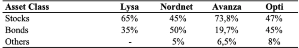
public information available, it is observable that the allocation strategies differ between the robo-advisors. Evidence of this is found in table 4:1 which shows the robo-advisors’ recommended portfolio allocations for an investor with a moderate risk profile. The underlying investment vehicles that are used in the portfolio compositions are presented in appendices 10-14. The robo-advisors’ proposed asset allocations are based on questionnaires used by each robo-advisor in the risk profiling process. To consistently estimate an investor with a moderate risk profile through the risk assessment process for all robo-advisors, a predetermined fictitious individual is used. Regarding subjective questions, the person is considered a risk neutral investor. Risk neutral implies that the investor is indifferent to risk when making investment decisions and therefor places himself or herself in the middle of the risk spectrum, focusing on expected return (Bodie et al, 2014). Regarding objective questions, the investor is 35 years old, has a gross income of 29,000 SEK per month and invests between 2000-5000 SEK each month in the robo-advisor.
Table 4:1, Robo-advisors’ recommended portfolios for a moderate investor. Recommended allocation between stocks, bonds and others.
As previously mentioned, robo-advisors have not been operating for a long time and therefor it is not possible to use the robo-advisors’ specific investment vehicles to assess the long-term performance. To determine and replicate the long-term performance of the robo-advisors, asset data with similar properties to the robo-advisors underlying investment vehicles are identified. This allows for portfolio replications of the robo-advisors’ portfolios with the same characteristics as the actual robo-advisors and makes it possible to recreate and execute the robo-advisors’ allocation strategies.
The equity part of the portfolios is decomposed by identifying the underlying investment vehicles used by each robo-advisor and the underlying indices that each investment vehicle tracks. The specifics are given in appendices 10-14. Based on the underlying indices that the vehicles track, each investment vehicle is categorised into an equity asset class.
31
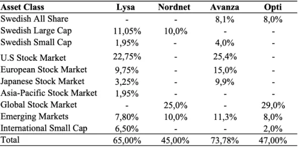
Each of the 10 asset classes under the equity part are represented by established indices. The indices used as asset classes are either underlying indices for the specific investment vehicles or indices with similar properties due to lack of historical data on the original indices. Table 4:2 presents the proposed equity allocation for an investor with a moderate risk profile.
Table 4:2, Robo-advisors proposed allocation for a moderate risk profile investor. Equity quota of the portfolio.
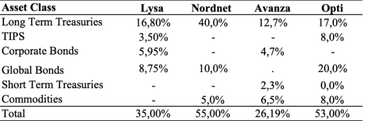
A different approach is used for constructing the non-equity portion of the portfolio. The specific bonds that are used by robo-advisors are categorised into different classes defined and categorised by Morningstar. Based on Morningstar’s classification, the different asset classes are represented by specific indices. Long term treasuries are represented by SHB Swedish All Bond Tradable index. This index has benchmark status and reflects the Swedish market for covered housing bonds and bonds issued by state and municipality (Handelsbanken, 2019)., Treasury inflation-protected securities (TIPS) are represented by S&P Sweden Sovereign Inflation-Linked Bond Index. The index is designed to track the performance of SEK-denominated inflation-linked securities (S&P Dow Jones Indices, 2019). Corporate bonds are represented by S&P Sweden Investment Grade Corporate Bond Index. This index tracks the performance of bonds issued by Swedish investment grade classified companies (S&P Dow Jones Indices, 2019). Global bonds are represented by PIMCO Global Bond Opportunity fund and tracks Bloomberg Barclays global aggregate (Morningstar, 2019). SHB Commodity index is used to represent commodities since all the robo-advisors actual commodity vehicles use SHB Commodity Index as underlying index (Handelsbanken, 2019). Handelsbanken Sweden repo tradable index is used for the short-term treasuries asset class. The index replicates an
32
investment in a fictitious loan at an interest rate corresponding to the Swedish central bank repo rate (Handelsbanken, 2019). The non-equity quota of the portfolios can be seen in table 4:3.
Table 4:3, Robo-advisors proposed allocation for a moderate risk profile investor. Non-equity quota of the portfolio.
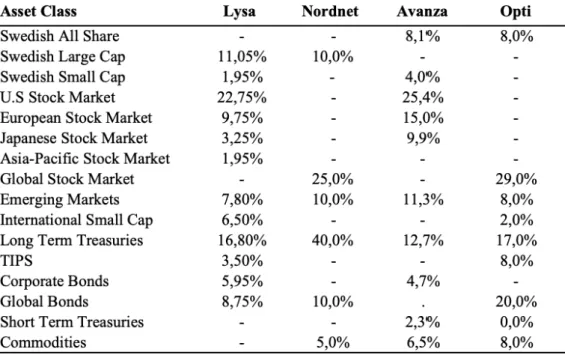
When the investment vehicles are categorised and decomposed into different asset classes, the asset classes are weighted into their respective portfolios. The process is the same for both the equity and the non-equity portion of the portfolio. The results from the final mapping and re-construction of the portfolios for a moderate investor are shown in table 4:4.
33
4.3 Asset Correlation
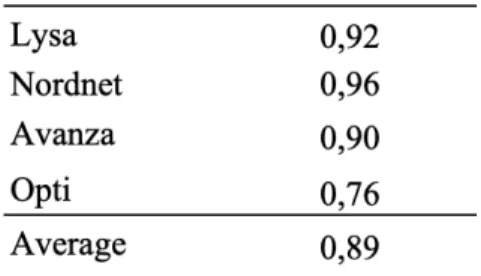
To ensure high quality and allowing for an accurate comparison of the investment vehicles representing each asset class in the constructed portfolios, an asset correlation analysis is done. The asset correlation analysis computes the Pearson correlation between the asset classes’ representative investment vehicles and the actual investment vehicles in the robo-advisors’ portfolios. In this research, the Pearson correlation is computed based on the assets monthly returns (Portfolio Visualizer, 2019). Pearson correlation measures the strength between two variables (or assets in this case) linear correlation. The value is between +1 and -1 where 1 is a total positive correlation. 0 means that there is no linear correlation at all and -1 means that there is a total negative correlation between the variables (Philip Sedgwick, 2012). Portfolio Visualizer’s correlation tool is used to calculate the correlation data for the replicated portfolios’ investment vehicles and the actual robo-advisors’ investment vehicles. Since the robo-advisors’ investment vehicles all have unique portfolio weights, a weighted Pearson correlation test is conducted to measure the overall portfolio correlation of the replicated portfolios.
Table 4:4, Robo-advisors proposed allocation for an investor with a moderate risk profile. All asset classes.
Table 4:4, Robo-advisors proposed allocation for an investor with a moderate risk profile. All asset classes
34
4.4 Benchmarks
Regarding the construction of appropriate and relevant benchmarks for the backtesting of each portfolio, two types of asset classes are used: Vanguard Total World Stock Market (VT) and PIMCO Global Bonds (PIGLX). These indices represent the asset classes that the robo-advisors' respective portfolios contain. To represent the equity part of the benchmark, given that the Swedish robo-advisors’ portfolios are diversified in a global way, Vanguard Total World Stock Market (VT) represents “holding the stock market”. The index represents the approximated return of all the stock markets, including large/small/mid-cap, emerging markets and developed markets.
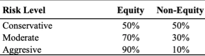
Representing the equity part of the benchmark, given that the robo-advisors invest in non-equity assets, PIMCO Global Bonds (PIGLX) represents ”holding the bond market”. To present the various risk profiles, data is used from American Association of Individual Investors (2017). The weights, or equity to non-equity ratio, represents the constructed benchmark for the conservative investor, moderate investor and the aggressive investor, shown in table 4:5
Table 4:5, Equity to non-equity ratio used in benchmark construction. Equity is represented by Vanguard Total Stock Market Index and non-equity is represented by PIMCO Global Bonds.
4.5 Backtesting
Portfolio Visualizer is used to backtest the performance of the re-constructed portfolios. The time horizon for the backtesting is from January 2010 to February 2019. The time frame used in this report is chosen based on the available data for the investment vehicles that the replicated portfolios are built upon. Due to lack of historical data older than 15 years the research is not able to assess the hypothetical performance during the financial crisis in 2007 and 2008.
35
Portfolio Visualizer is a software platform with quantitative and factor-based investment tools, for example backtesting portfolio allocations and portfolio optimisations (Portfolio Visualizer, 2019). The research is conducted with a fictitious portfolio with a starting balance of 10,000 SEK which is invested in the replicated portfolios from the selected robo-advisors.
Portfolio Visualizer’s backtesting tool calculates portfolio returns, such as end balance and Compounded Annual Growth Rate (CAGR) based on monthly asset returns. The risk characteristics of the portfolios, in this case standard deviation, Sharpe ratio and Sortino ratio, are calculated from monthly returns and annualized. The risk-free rate used in this backtesting is the historical U.S. 1-month T-bill return data. The U.S. risk free rate is used due to limitations in the Portfolio Visualizer software, making it non available to use the Swedish risk-free rate. According to the robo-advisors framework and modern portfolio theory rebalancing bands are also supported. The rebalancing bands are based on 5 per cent absolute deviation from the target allocation, or 25 per cent relative deviation from the target allocation, mapped by the allocation from the replicated portfolios, see table 4:4.
4.6 Efficient Frontier
The efficient frontier shows the return and risk curve for a mix of selected assets that minimize the portfolio risk. Portfolio risk is defined in terms of volatility given expected return (Markowitz, 1952). To calculate the efficient frontier, data from the 16 asset classes, presented in table 4:4 are used. These asset classes are used in the MVO to calculate and obtain the efficient frontier based on historical performance. By using Portfolio Visualizer output data, the asset class correlation matrix, expected return and the standard deviations are acquired. The same time-frame used for backtesting the portfolios, 2010 to 2019, is applied to calculate the efficient frontier. Standard deviations and expected returns in the efficient frontier are annualized from the monthly returns (Portfolio Visualizer, 2019).
The efficient frontier is constructed in line with Swensen’s (2009) research on estimation error in MVO where asset class weight constraints are added to ensure diversification. In this research, weight constraints are added to the efficient portfolios limiting portfolio assets to have a maximum occupancy of 30 per cent of the portfolio quota. Non-negativity constraints are added to prohibit short positions in the portfolio. In addition to these constraints a 10 per cent maximum in commodities and short-term treasuries is applied. These conditions are applied
36
due to the actual robo-advisors’ portfolios only holding a maximum 10 per cent in commodities and short-term treasuries.
4.7 Estimating Net Returns
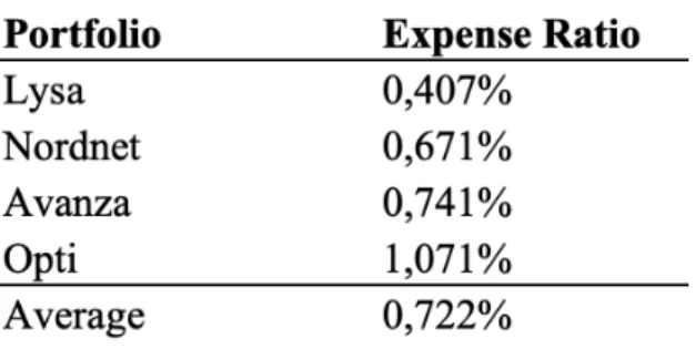
To estimate the net returns for the robo-advisors in this research, the gross returns from backtesting the allocation from table 4:4 are obtained, followed by subtracting the expenses from the portfolios gross returns. Expenses associated with each of the four robo-advisors are calculated by taking the annual management fees and adding expense ratios from the underlying investment vehicles according to their respective quota of the portfolio. For the robo-advisors that trades with ETFs there are no trading commissions added due to the fact that these costs occur when ETFs are sold or bought. In this research, this situation only occurs when rebalancing portfolios, however robo-advisors include free rebalancing as the cost is calculated as part of the annual management fees. The expense ratio of each robo-advisor is shown in table 4:6. Appendices 6-9 portrays a more detailed picture of the expense ratios for each investment vehicles.
Table 4:6, Expense ratios for the robo-advisors replicated in this research. Expense ratios are constructed from management fees and underlying investment vehicles’ expense ratios.
The benchmark’s cost structure is calculated by summing up the robo-advisors’ management fees and taking the average of this sum to represent the benchmark's management fee. The expense ratio of the equity part of the benchmark is constructed by taking the average cost of all underlying investment vehicles in the equity part of the portfolio. The non-equity part of the benchmark is constructed by taking the average cost of all the non-equity investment vehicles. For the sake of simplicity annual re-balancing is assumed to not incur transaction costs. Table 4:6 shows the constructed benchmark’s expense ratio as “average”.