Nonconforming rotated Q1 tetrahedral element with explicit time stepping for elastodynamics

JTH R

R

2011:04

N

ONCONFORMING

R

OTATED

Q

T

ETRAHEDRAL

E

LEMENT WITH

E

XPLICIT

T

IME

S

TEPPING FOR

E

LASTODYNAMICS

P

H

A Survey of High Level Test Generation

Methodologies and Fault Models

Tomas Bengtsson and Shashi Kumar

ISSN 1404 – 0018

Research Report 04:5

D

M

E

J

U

SE-551 11 J

time-stepping for elastodynamics

Peter Hansbo

Department of Mechanical Engineering, Jönköping University, SE-55111 Jönköping, Sweden.

SUMMARY

In this paper we apply a rotated bilinear tetrahedral element recently introduced by Hansbo [1] to elastodynamics in R3. This element performs superior to the constant strain element in bending and, unlike the conforming linear strain tetrahedron, allows for row-sum lumping of the mass matrix. We study the effect of different choices of approximation (pointwise continuity versus edge average continuity) as well as lumping versus consistent mass in the setting of eigenvibrations. We also use the element in combination with the leapfrog method for time domain computations and make numerical comparisons with the constant strain and linear strain tetrahedra.

KEY WORDS: Finite element method, nonconforming element, explicit time stepping.

1. INTRODUCTION

In [1], we introduced a nonconforming Rotated Bilinear Tetrahedral (RBT) element, derived from the nonconforming hexahedral element introduced by Rannacher and Turek [2]. The RBT element has properties similar to the hexahedral element: improved bending behavior compared to the Constant Strain Tetrahedron (CST), as well as allowing for under-integration in near incompressibility. The shortcomings of the CST element are well known and attempts to improve its properties has typically employed mixed (stabilized) formulations with pressure or stresses as auxiliary variables, as in the Characteristics Based Split (CBS) algorithm of Zienkiewicz et al. [3, 4], or the nodal averaging (NA) approach of Bonet et al. [5, 6, 7], or the sub-grid stabilization method of Cervera et al. [8]. While the CBS approach only addresses near incompressibility, the NA approach additionally gives improved bending behavior. In contrast, the RBT element inherits these properties from its relation with the hexahedral element. No additional variables are introduced, no stabilization necessary, and symmetric solvers such as conjugate gradients can be employed in the stationary case. For explicit solvers, the natural (in the sense that it corresponds to a quadrature method, cf., e.g., Hansbo [9]) mass lumping method based on putting the row-sum in the diagonal of the lumped mass matrix can be used (which is not the case for the conforming linear strain tetrahedron).

An outline of the paper is as follows: in Section 2 we recall the RBT element and discuss two types of continuity imposed on the solution. In Section 3 we give application to the problem of linearized elastodynamics, with mass lumping. Finally, in Section 4 we give some numerical examples to show the properties of the approximation.

2. THE ROTATED Q1APPROXIMATION

In order to define a low order approximation which is stable for Stokes problem, Rannacher and Turek [2] constructed a hexahedral element with nodes on the faces. On the reference hexahedron in Fig. 1, we indicate the local numbering of degrees of freedom for this element. Two different kinds of continuity can now be imposed: point-wise continuity and average continuity (we remark that for the classical Crouzeix-Raviart nonconforming tetrahedral element [10], this is in fact the same thing).

On the reference element ˆK (for 0 ∑ ª,¥,≥ ∑ 1) we define the shape functions by

¡_i= a0+ a1ª+ a2¥+ a3≥+ a4(ª2° ¥2) + a5(ª2° ≥2).

For each shape function, this gives six unknowns a0–a5 for the six faces of a hexahedron

element. (It may seem that symmetry requires an additional term a6(≥2° ¥2); note, however,

that this term is represented by setting a5= °a4).

Enforcing point-wise continuity in the center of the faces, we immediately obtain

¡₁=1 3(2 +2ª°7¥+2≥°2ª2+ 4¥2° 2≥2), ¡₂=1₃(°1°ª+2¥+2≥+4ª2° 2¥2° 2≥2), ¡₃₌1 3(°1+2ª°¥+2≥°2ª2+ 4¥2° 2≥2), ¡₄₌1 3(2 °7ª+2¥+2≥+4ª2° 2¥2° 2≥2), ¡₅=1 3(2 +2ª+2¥°7≥°2ª2° 2¥2+ 4≥2), ¡₆=1₃(°1+2ª+2¥°≥°2ª2° 2¥2+ 4≥2).

In [1], we made the observation that there is a reference tetrahedron ˆT inscribed in the reference hexahedron ˆK, shown in Fig. 2. Using a a sub-parametric map F : (ª,¥,≥) ! (x, y, z), based on

the shape functions of the P1_{tetratedron, to a physical tetrahedron T, we map mid side nodes}

in the reference configuration to mid side nodes in the physical configuration (an isoparametric map gives the same result). This means that the mapping will be affine and we have a first approximation scheme in the physical configuration. We can also define a second set of shape functions {√i(x)} with edge-wise mean continuity in physical space, defined by setting, on an

element T, 1 |Ei| Z Ei √_j(x) ds =Ω 1 if i = j, 0 if i 6= j.

Here Eiis the edge, of length |Ei|, associated with local node i, i = 1,...,6.

To formalize the finite element method, let Th := {T} be a conforming, shape regular

tetrahedrization of ≠Ω R3 and Eh the set of all element edges in the mesh. We can then

introduce non-conforming finite element spaces constructed from the basis previously discussed by defining the two variants

with midpoint continuity, and

V₂h:= {v : v|T± F 2 QR1( ˆT), 8T 2 Th;

Z

Ev ds is continuous, 8E 2 Eh}, (2)

with mean continuity along the edges. 3. APPLICATION TO ELASTODYNAMICS

3.1. Problem formulation and finite element approximation

We consider the equations of linear elasticity describing the deformation of an elastic body occupying a domain ≠ in R3 during a time interval (0, tmax): find the displacement u(x, t) =

[ui(x, t)]3_i=1and the symmetric stress tensor æ =£æ_{i j}§3_{i, j=1}such that

8 > > > > > > > > > > > > > > > < > > > > > > > > > > > > > > > : æ _{= ∏ r · uI + 2µ"(u) in}≠£ (0, tmax), %@ 2_u @t2 ° r · æ = f in≠£ (0, t max_), u = 0 on @≠_D£ (0, tmax), n ·æ = h on @≠_N£ (0, tmax), u(x,0) = u0(x) in≠, @u @t(x,0) = w0(x) in≠. (3)

Here "(u) =£"_{i j}(u)§3_{i, j=1}is the strain tensor with components

"_{i j}(u) =1 2 µ @u_i @x_j + @u_j @x_i ∂ , r · æ =hP3_j=1@æ_{i j}/@x_ji3 i=1,I = £

±_{i j}§3_{i, j=1}with ±_{i j}= 1 if i = j and ±i j= 0 if i 6= j, f and h are given

loads, andn is the outward unit normal to @≠. Furthermore, % is the density and ∏ and µ are

the Lamé constants. In terms of the modulus of elasticity, E, and Poisson’s ratio, ∫, we have that

∏= E∫/((1 + ∫)(1 ° 2∫)) and µ = E/(2(1 + ∫)). Finally, u0 andw0are given initial displacements

and velocities, respectively. Introducing the space

W := {v : v 2 [H1(≠)]3,v is zero on @≠D},

the weak form of (3) can be written: findu 2 W such that

µ %@ 2_u @t2,v ∂ ≠+ a(u, v) = (f , v)≠+ (h, v)@≠N 8v 2 W, (4) where a(u,v) :=Z ≠ æ(u) : "(v) dV, (5)

where æ : ø =Pi jæ_{i j}ø_{i j}denotes tensorial contraction, and (·,·)_S denotes the L₂ scalar product

To define the finite element method, we introduce the non-conforming finite element space constructed from the spaces Vh

i in (1)–(2) by defining

W₁h:= {v : v 2 [V1h]3,v is zero at the midpoints of edges on @≠D},

and

W₂h:= {v : v 2 [V2h]3,

Z

Ev ds is zero at the edges on @≠D}.

The (semi-discrete) finite element method is to finduh2 W_ihsuch that

µ %@ 2_u h @t2 ,v ∂ ≠+ ah (uh,v) = (f ,v)≠+ (h, v)@≠N 8v 2 Wih, i = 1or 2. (6) Here ah(u,v) := X T2Th Z Tæ(u) : "(v) dV (7)

has to be written as a sum over the elements due to the nonconformity of the approximation. The convergence and stability of this method follows from the analysis in [1].

We shall also consider the discrete time-harmonic eigenvalue problem of findinguh2 W_ihand

!2 R+_{such that}

ah(uh,v)°!2(%uh,v)≠= 0 8v 2 W_ih, i = 1or 2. (8)

This eigenvalue problem is of interest in itself, but will here only be used in order to ascertain the apparent stiffness of different methods.

3.2. Mass lumping

For the time dependent problem, we end up with a matrix system of the type

Md2u

dt2 + Su = f, (9)

and for the eigenvalue problem

°

S°!2_M¢_{u = 0,}

whereS is the stiffness matrix and M is the mass matrix. For explicit time stepping schemes,

it is important that the mass matrix can be lumped to a diagonal matrix ML_{. The basic}

idea of mass lumping is to use an integration scheme approximating the integrand with the shape functions in use (see [9]). Thus, for Vh

1 the integral over T of a given function f (x) is

approximated Z Tf (x) dV º 6 X i=1 Z T'i(x)f (xi) dV = 6 X i=1Wif (xi), where Wi:= Z T'i(x) dV.

Replacing f (x) by the integrands of the mass matrix, 'j(x)'k(x), we see by the properties of the

the diagonal. The integral of a shape function can also be found by summing the corresponding row in the full mass matrix (row-sum lumping), since

X j Z ≠ '_i'_jdV = Z ≠ '_iX j '_jdV

and Pj'j= 1. The weights Wi are thus immediately obtained given the full mass matrix. For

Vh

2 the situation is slightly more complicated. If we define the mean value of f (x) along edge Ei

by º_0,if := 1 |Ei| Z Ei f (x)ds

we can make the approximation f (x) ºP6

i=1√i(x)º0,if , which we note is exact if f 2 V2h, and

Z Tf (x) dV º 6 X i=1 Z T√i(x)º0,if dV.

Setting now f = √j√k, we have

Z T√j√kdV º 6 X i=1 µZ T√idV 1 |Ei| Z Ei √_j√_kds ∂ ,

which does not yield a diagonal matrix. We thus make an additional assumption: Z

Ei

√_j√_kds º

Z

Ei

√_jº_0,i√_kds = |E_{i| º0,i}√_jº_0,i√_k=

Ω

|Ei| if i = j = k,

0 otherwise.

We note that this would be exact if √ were linear (cf. the Crouzeix-Raviart element in 2D [10]). The resulting lumped mass matrix thus also has entries of the type

˜ Wi=

Z

T√i(x) dV

and these can be taken from the row sum of the corresponding full mass matrix, since 1 = P

i√iº0i1 =Pi√i.

The entries in the diagonal of the lumped element mass matrices are given explicitly by Wi= ˜Wi= |T|/6, where |T| denotes the volume of T. Since one point integration per element,

using derivative information, cf. [11], can be used for evaluating the stiffness matrix (and, since the mapping is affine, is indeed exact assuming constant material data), the implementation of the RQT element can be made competitive with the CST element.

Remark 3.1. It may seem like an unnecessary complication to introduce mean edge continuity

because it seems nothing is gained in comparison with point-wise continuity. One benefit lies in that, just like a discrete version of Gauss’ theorem is gained for face continuity in the Rannacher– Turek element, cf. [2], we retrieve a discrete version of Stokes’ theorem with edge continuity. That is, for a given displacement fieldu we have an edge interpolant º0u (of edge wise mean values of

u) such that for a face F on the tetrahedron,

Z FnF· (r £ u) dA = I @Fu · dr = I @F º₀u · dr = Z FnF· (r £ º0u) dA,

where nF is a unit normal to F and dr follows the right-hand rule. Thus the edge oriented

method has additional structure (giving bending resistance) built into it, and can be expected to be stiffer than the point oriented method (which, experiments show, tends to underestimate the actual stiffness). This will be further commented in the numerical examples below.

3.3. Time stepping

For the explicit time stepping, we use the “position Verlet" version of the leapfrog method applied to (9), i.e., for equidistant time stepping with step size k = tn+1° tn, and withunº u(tn) and

vnº du(tn)/dt, we solve, for n = 0,1,...,nmax(where tmax= k nmax),

un+1/2= un+k₂vn,

MLvn+1= MLvn+ k (f(tn+1/2) °Sun+1/2),

un+1= un+1/2+k₂vn+1.

As is well known, cf., e.g., [12], this requires a time step size k ∑ 2/!max, where !maxis computed

from the eigenvalue problem°S°!2_ML¢_{u = 0.}

4. NUMERICAL EXAMPLES 4.1. Eigenfrequencies

We consider a problem analyzed in [13], consisting of a hexahedron with side lengths Lx, Ly,

and Lzalong the corresponding axes, with slip boundary conditions on each side (i.e., with the

normal displacement prescribed to zero on each face of the cube). Assuming constant material data, the eigenvalues are then given analytically by

!2= ª_{2%(1 +∫)(1°2∫)}E where, with Æ_n=nº Lx, Øn= nº Ly, ∞n= nº Lz, n = 0,1,...,

we obtain a set of eigenvalues associated with solenoidal modes:

ªs_{i jk= (1 ° 2∫)(Æ}2_{i+ Ø}2_{j+ ∞}2_k),

and another set of eigenvalues associated with compressive modes:

ªc_{i jk= 2(1 ° ∫)(Æ}2_{i+ Ø}2_{j+ ∞}2_k), with i + j + k 6= 0.

The multiplicity of the eigenvalues is also given in [13]. We set % = 7850 kg/m3_{, E = 200 GPa,}

and ∫ = 0.33, and compare the convergence of the lowest eigenvalue for the point oriented, edge oriented, and CST element, with and without mass lumping, in Fig. 4. The point oriented approximation gives the smallest error, and the CST element is the stiffest. Note that we are measuring the error with respect to degrees of freedom (NDOF). In Fig. 5 we give the quotient of the exact eigenvalue to the approximate, and we note that the point-oriented method (with lumping) may underestimate the eigenvalue. This is unlike a standard conforming FEM, where the eigenvalues are guaranteed to be over-estimated.

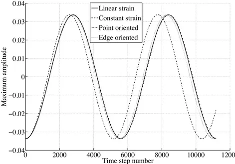
4.2. Explicit time stepping

We consider free vibration in different modes: compressive, bending, and twisting. The domain is a console of dimension (0,1)£(0,0.1)£(0,0.1), fixed at x = 0. The compression mode is obtained by releasing the displacements corresponding to a volume load f = (°1011_{,0,0), Fig. 6, the}

bending mode corresponds to the lowest eigenvector, Fig. 8, and the twisting mode is obtained by releasing the displacements corresponding to f = (0,°1011_{(z ° 0.05),10}11_{(y ° 0.05)), Fig. 10.}

The deformation plots also give information about the mesh used.

The different initial conditions are computed using the linear strain tetrahedron, and the solution is transferred to the nodes of the linear polynomials and the rotated Q1polynomials for

comparison. Thus similar starting conditions is used for each of the three elements. We compare time plots for the different cases using the same time step (the critical time step computed for the linear strain tetrahedron) over a few periods. The material data are the same as previously. Note that the linear strain tetrahedron cannot be lumped and thus does not allow for a fully explicit scheme; we useM in the place of ML_{for this element.}

In Fig. 7 we see that for pure compression, all approximations give essentially the same result. For bending, Fig. 9, the constant strain tetrahedron exhibits a marked period shortening due to its spurious bending stiffness. The edge oriented approximation is slightly stiffer, and the point value oriented is slightly more flexible, than the linear strain tetrahedron, as expected. The situation is the same, only more pronounced, in the twisting case, Fig 11.

5. CONCLUDING REMARKS

The rotated Q1 tetrahedron element allows for two different approximations: one point value

oriented, with continuity in the midpoint of the edges, and one edge oriented, with mean values along the edges as unknowns. Both approximations allow for mass lumping. Numerically we observe a slightly overly flexible response, compared to the linear strain element, for the point-oriented method, and a slightly overly stiff response for the edge-point-oriented. Both approximations perform distinctly better than the constant strain element in bending dominated situations.

REFERENCES

1. Hansbo P. A nonconforming rotated Q1approximation on tetrahedra. Computer Methods in Applied Mechanics

and Engineering 2011;200(9-12):1311–1316.

2. Rannacher R, Turek S. Simple nonconforming quadrilateral Stokes element. Numerical Methods for Partial Differential Equations 1992;8(2):97–111.

3. Zienkiewicz O, Rojek J, Taylor R, Pastor M. Triangles and tetrahedra in explicit dynamic codes for solids. International Journal for Numerical Methods in Engineering 1998;43(3):565–583.

4. Rojek J, Oñate E, Taylor R. CBS-based stabilization in explicit solid dynamics. International Journal for Numerical Methods in Engineering 2006;66(10):1547–1568.

5. Bonet J, Burton A. A simple average nodal pressure tetrahedral element for incompressible and nearly incompressible dynamic explicit applications. Communications in Numerical Methods in Engineering 1998;

14(5):437–449.

6. Bonet J, Marriott H, Hassan O. An averaged nodal deformation gradient linear tetrahedral element for large strain explicit dynamic applications. Communications in Numerical Methods in Engineering 2001;17(8):551–561.

7. Bonet J, Marriott H, Hassan O. Stability and comparison of different linear tetrahedral formulations for nearly incompressible explicit dynamic applications. International Journal for Numerical Methods in Engineering 2001;

8. Cervera M, Chiumenti M, Codina R. Mixed stabilized finite element methods in nonlinear solid mechanics Part I: Formulation. Computer Methods in Applied Mechanics and Engineering 2010;199(37-40):2559–2570.

9. Hansbo P. Aspects of conservation in finite element flow computations. Computer Methods in Applied Mechanics and Engineering 1994;117(3-4):423–437.

10. Crouzeix M, Raviart PA. Conforming and nonconforming finite element methods for solving the stationary Stokes equations. I. Revue Française Automatique Informatique Recherche Opérationnelle Série Rouge 1973;7(R-3):33–75.

11. Hansbo P. A new approach to quadrature for finite elements incorporating hourglass control as a special case. Comput. Methods Appl. Mech. Engrg. 1998;158(3-4):301–309.

12. Bathe KJ, Wilson EL. Numerical Methods in Finite Element Analysis. Prentice-Hall Inc., 1976.

13. Day D, Romero L. An analytically solvable eigenvalue problem for the linear elasticity equations. Technical Report SAND2004-3310, Sandia National Laboratories 2004.

ζ ξ η 1 4 2 5 6 3

Figure 1. Reference hexahedron ˆK.

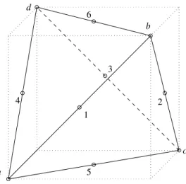
1 4 2 5 6 3 a b c d

1 2 3 4 5 6 a c b d

Figure 3. Physical element T.

6 5 4 3 2 1 1.5 2 2.5 3 3.5 4 4.5 5 5.5 6 6.5 log(1/NDOF1/3)

log(Error) Point, full

Point, lumped Edge, full Edge, lumped CST, full CST, lumped

4

3.5

3

2.5

0.92

0.94

0.96

0.98

1

1.02

log(1/NDOF

)

Exact/Approximate

Point, full

Point, lumped

Edge, full

Edge, lumped

CST, full

CST, lumped

Figure 5. Quotient between exact and approximative first eigenvalue.

0 200 400 600 800 1000 1200 1400 1600 1800 0.08 0.06 0.04 0.02 0 0.02 0.04 0.06 0.08

Time step number

Maximum amplitude

Linear strain Constant strain Point oriented Edge oriented

Figure 7. Response for compression mode.

0 2000 4000 6000 8000 10000 12000 0.04 0.03 0.02 0.01 0 0.01 0.02 0.03 0.04

Time step number

Maximum amplitude

Linear strain Constant strain Point oriented Edge oriented

Figure 9. Response for bending mode.

0

500

1000

1500

2000

2500

3000

0.015

0.01

0.005

0

0.005

0.01

0.015

Time step number

Maximum amplitude

Linear strain

Constant strain

Point oriented

Edge oriented