Tomographic reconstruction of subchannel void measurements of nuclear fuel geometries

(1)

UPTEC F15007

Examensarbete 30 hp

Mars 2015

Tomographic reconstruction of

subchannel void measurements of

nuclear fuel geometries

(2)

Teknisk- naturvetenskaplig fakultet UTH-enheten Besöksadress: Ångströmlaboratoriet Lägerhyddsvägen 1 Hus 4, Plan 0 Postadress: Box 536 751 21 Uppsala Telefon: 018 – 471 30 03 Telefax: 018 – 471 30 00 Hemsida: http://www.teknat.uu.se/student

Abstract

Tomographic reconstruction of subchannel void

measurements of nuclear fuel geometries

Magnus Ahnesjö

The Westinghouse FRIGG loop in Västerås, Sweden, has been used to study the distribution of steam in the coolant flow of nuclear fuel elements, which is known as the void distribution. For this purpose, electrically heated mock-ups of a quarter BWR fuel bundles in the SVEA-96 geometry were studied by means of gamma tomography in the late 1990s. Several test campaigns were conducted, with good results, but not all the collected data was evaluated at the time.

In this work, tomographic raw data of SVEA-96 geometry is evaluated using two different tomographic reconstruction methods, an algebraic (iterative) method and filtered back-projection. Reference objects of known composition (liquid water) are used to quantify the decrease in attenuation arising from the presence of the void, which is used to create a map of the void in the horizontal cross sections of the fuel at various axial locations. The resulting detailed void distributions are averaged over subchannels and the subchannel steam core for comparison with simulations. The focus of this work is on the void distribution at high axial locations in the fuel, in fuel bundles with part-length fuel-rods. Measurements in the region above the part-length rods are compared with simulations and the reliability of each method is discussed. The algebraic method is found to be more reliable than the filtered back-projection method for this setup. A reasonable agreement between measurements and predictions is shown. The void, in both cases, appears to be slightly lower in the corner downstream the part-length rods.

ISSN: 1401-5757, UPTEC F15 007 Examinator: Tomas Nyberg Ämnesgranskare: Peter Andersson Handledare: Stig Andersson

(3)

Sammanfattning

I kärnkraftverk av kovattenreaktormodell finns vatten i ett tvåfasflöde. Det är viktigt att veta

fördelningen av ånga i detta flöde eftersom vattnet är moderator och ånga sänker därmed reaktiviteten i reaktorn, samtidigt måste bränslet alltid vara täckt av flytande vatten för att tillgodose kylning.

Fördelningen av ånga i tvåfasflödet kallas void och är volymfraktionen av ånga. Att undersöka voiden i en reaktor under operation är opraktiskt då det är en mycket svår miljö att utföra mätningar i. Därför undersöks void och kritiskt värmeflöde med elektriskt upphettade stavar utanför reaktorn, i

testanläggningar vars geometri motsvarar kärnbränsle geometrin. Vid FRIGG i Västerås gjordes void mätningar med gamma tomografi under slutet av 90-talet. I tomografi mäts det, genom ett objekt, transmitterade gammat i ett antal projektioner som sedan kombineras för att återskapa en bild av objektet. Mätningarna gjords på ett simulerat fjärdedels-knippe med dellånga stavar precis nedströms den övre änden av de dellånga stavarna. Det området är av intresse för validering av beräkningskoder då det finns mycket få mätningar gjorda på sådana geometrier.

Två rekonstruktionsmetoder, en algebraisk metod och filtered back-projektion, har implementeras i MATLAB. Svårigheter på grund av storleken på testanläggningen och begräsningar hos mätutrustningen har blivit bemött, främst med användning av referensmätningarpå kända geometrier. Tvåfasmätningar av voiden gjordes kopplad till referensmätningar på låg effekt och med vatten nära kokpunkten. Med hjälp av referensmätningar kunde en attenueringsskillnad, som är proportionell mot voiden, mellan de två fallen beräknas. Referensmätningar gjordes också med kallt vatten och kall luft. Dessa mätningar användes för att utvärdera de två rekonstruktionsmetoderna där den algebraiska metoden valdes som den mest tillförlitliga av de två.

Från de rekonstruerade void distributionerna beräknades medelvoiden i varje delkanal. En delkanal är definierad som området begränsat av de minsta avståndeten mellan fyra stavcentrum. På grund av hög brusnivå testades tre stycken beräkningsmönster för att beräkna medelvoiden. En jämförelse med simuleringsresultat gjordes och en rimlig överenstämmelse mellan mätdata och simuleringar kunde påvisas. Gemensamt för simuleringar och mätdata var att delkanal medelvoiden var något lägre i området nedströms de dellånga stavarna.

(4)

2

1 Introduction

1.1 Nuclear power

With a worldwide increase in energy demand there is a necessity for low carbon energy supply. Nuclear power plants use the energy stored in matter to generate electricity and therefore have a very low carbon footprint. In nuclear power plants the energy stored in the nuclei of uranium is released as heat through a series of nuclear interactions. The energy release is used to boil water to be used in steam turbines. There are several ways the heat from the nuclear reactions can be extracted, for the most common type of nuclear power plants, light water reactors, two similar designs are used: Boiling water reactor (BWR) and pressurized water reactor (PWR). In BWRs the water boils directly in the reactor core, while in PWRs a primary loop circulates high pressure liquid water through the core, which in turn boils water in a secondary loop to which a steam turbine is connected. Of Sweden’s ten currently operational reactors, seven are BWRs and three are PWRs and they produced 61 TWh of electricity during 2012 [1]. During operation of a BWR the water is in a two-phase condition in the core, which creates equilibrium in the operating conditions due to the fact that water acts both as a moderator and a coolant. A consequence is that if the reactivity is high the heat flux increases, which in turn produce more steam which lowers the reactivity, thereby stabilizing the power output of the reactor. However, it is still important to have detailed knowledge and predictive capability of the production and transport of steam in the core. For example, if the heat flux from the fuel rods becomes too high all the water will boil away on the fuel surface, a so called dry-out, and the cooling of the rods will be lost and they risk damage. Safety margins (dry-out margins) to avoid such events have been determined from testing facilities like the FRIGG-loop. Likewise, it is of importance to have ability to shut down the reactor at all times during operation. Therefore, the shut-down margins are calculated, i.e., the amount of reactivity below criticality resulting from the insertion of the control rods. For the calculation of the shut-down margin, knowledge of the moderation efficiency, which is governed by the amount of liquid water present, is needed.

1.2 Void

One important property for the operation of a BWR is the void distribution. Void fraction is a measure of the volume fraction of steam in a two phase flow, i.e., the void fraction is α=0 for liquid water and α=1 for saturated steam (1-1).

𝛼 =

𝑉𝑠

𝑉𝑇

,

where 𝑉𝑠 is the volume of the steam and 𝑉𝑇 is the total volume occupied by the steam and water. By

substituting volume with density the void can then be described as 𝜌_𝑇 =𝑚𝑇 𝑉_𝑇 = 𝑚_𝑠 (𝑉𝑠 𝛼 ) + 𝑚𝑤 ( 𝑉𝑤 1 − 𝛼) = 𝛼𝜌_𝑠+ (1 − 𝛼)𝜌_𝑤 ⟺ 𝛼 =𝜌𝑤− 𝜌𝑇 𝜌_𝑤− 𝜌_𝑠

where m is the mass of the total (T), steam (s) and water (w) respectively. Since the attenuation of a material is directly proportional to the density, 1-2 becomes

𝛼 =𝜇𝑤− 𝜇𝑇 𝜇_𝑤− 𝜇_𝑠

Where 𝜌 stands for density and 𝜇 stands for the linear attenuation coefficient, i.e., the damping of the radiation per unit length travelled.

It is important to know the void distribution inside a BWR as it affects both the dry-out and shut down margins. Knowledge of the void is also important for nuclear fuel design and in-core fuel management,

1-1

1-2

(7)

5

because of its implications on the cooling efficiency and the reactivity. A subchannel analysis code [2] can be used to calculate the void for various fuel geometries.

1.3 The FRIGG loop

The FRIGG loop is an electrically heated test loop located in Västerås owned by Westinghouse Electric AB. The loop is used to simulate the thermal-hydraulic conditions of BWR fuel bundles. A test loop is very useful since it can be used for experiments that would be impossible to do in real nuclear power plants for safety reasons, such as studies of thermal-hydraulic conditions close to the critical heat flux. The FRIGG loop was constructed in 1966 and has been improved over the years to include a larger variety of testing conditions and measurement equipment for different physical properties. Among other things, the loop was used to empirically find a relative radial power distribution that minimizes the risk for dry-out in a single subchannel. This is referred to as the optimal power distribution. The FRIGG loop also has the ability to test different axial power distributions that simulate the expected power

distribution in nuclear fuel.

1.4 Fuel geometry history

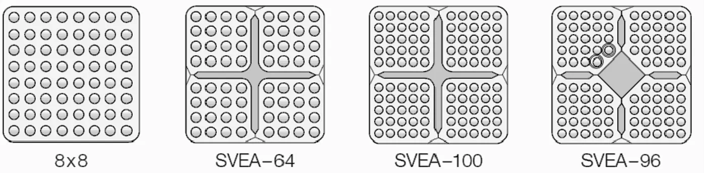
The development of fuel assemblies for BWR has gone from simple 8x8 rectangular fuel bundles to the SVEA-96 design (Figure 1-1) through a number of iterations. However, the empirical void correlations that originally had been developed in the 1960s [3] was for the older geometry and therefore a new measurement campaign was needed in order to assure the correctness of the calculations of the safety margins. Therefore a void measurement campaign was performed in the 1990s, where both average void distributions and detailed void distributions were measured. However, although some results were published [4], all measured data was not analyzed at the time. This includes in particular the detailed void distributions and subchannel void in fuel bundles with part-length rods, i.e., fuel rods in the outer corners of the bundles that have a shorter axial length than the rest of the fuel.

Figure 1-1 Four fuel designs in development of SVEA-96 which is the design used today. The fuel rods have become smaller and

increased in number and the fuel bundle has been divided into four sub-bundles. The part length rods in SVEA-96 are marked in one sub bundle by . Images from [3].

1.4.1 Part length rods

Part length rods are used because they improve shut down margins and reduce assembly pressure drops. Since the neutron flux is much higher in the center of the bundle, especially if there are rods close to the center, a more uniform distribution of thermal neutrons is achieved by using part-length rods. The part length rods also gives a benefit to the axial power distribution as the neutron flux is lowered in top of the bundle where it is better to have low power and maintain high power lower in the bundle. By having part-length rods a higher utilization of the fuel and a higher burn up ratio can be achieved.

(8)

6

1.5 Tomography

Tomographic imaging is used in a wide variety of fields, most prominently in medicine. Tomography is a non-intrusive method to image the inside structures of an object. A common type is X-ray computed tomography in which X-rays are emitted from a source to irradiate the object under investigation and sensors register the intensity of the transmitted X-rays. The source and sensors can rotate around the object and a large number of projections can then be combined to reconstruct the spatially resolved attenuation image in either in 2D or 3D. The technique is very useful in order to picture objects without intrusion, which might otherwise destroy or change the conditions inside the object. There are several mathematical approaches, two of which are algebraic reconstruction and filtered back-projection. Two common examples of measurement geometries are fan-beam, from one source-point, with sensors set in an arc, and parallel beam geometry where all sources and all sensors are located on two

corresponding lines ( Figure 1-2).

1.6 Scope of work

The aim of this work was to do an implementation and comparison of tomographic reconstruction algorithms for measurements using gamma transmission on nuclear fuel geometries. The implemented algorithms should be used to reconstruct all of the detailed void measurements done at the FRIGG loop. The primary focus was on the measurements done on geometries with part length rods especially measurements done downstream of the end of the part length rods. From the reconstructed

measurements the average void in the subchannels would be calculated and for validation purposes be compared with the result from a subchannel analysis code (VIPRE-W).

2 Tomographic void measurement at Frigg

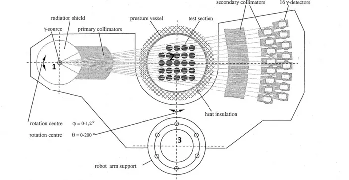
2.1 Tomographic measurement equipment and configuration

The tomographic measurements carried out at FRIGG were done with a 137Cs gamma source and a detector board [4]. The gamma radiation from 137Cs has the energy 662 keV. 16 detectors were attached in two rows, and cooling system was used to keep them at constant temperature of 19°C.

Figure 1-2 Concept of a fan-beam geometry (left) and a parallel beam geometry (right). 𝜽 and 𝜽𝒑 are the projections angles for the two geometries. 𝝋 and 𝒅 are the locations of the sensor

beams in regards to the center beam given as angle and length respectively .

𝜃𝑝

d

𝜃 𝜑

(9)

7

The detector board was transported around the pressure vessel by a robot arm. The pressure vessel had rings to which the robot orientated to find the positions. Due to the weight of the detector board the robot could not maintain its internal coordinate system as the further the arms were elongated the further it dropped its position from the programed route. Therefore, an optic servo system was set in place and compensation was made in the robot program.

2.1.1 The detector

The 16 detector elements used in the detector setup were bismuth germanate (BGO) detectors, which are scintillators. A scintillator material emits photons when irradiated by ionizing radiation and the emitted photons are then converted to electric signals through an electronic light sensor, which in this case are photomultiplier tubes. The electrical response of the detector is proportional to the energy deposited by the gamma quanta. The energy deposition by the gamma is determined by its three interaction types, photoelectric absorption where all the energy of the gamma quanta is absorbed, pair production and Compton scattering where the gamma quanta only deposits part of its energy in the BGO crystal. For 137Cs, pair production does not occur since the gamma quanta energy is less than twice the electrons rest energy (2*511 keV). Channels count events corresponding to energy deposited which from a distribution around 662 keV. The numbers of counts in the full energy peak was then registered. The registered intensity therefore also contains some background radiation, counts of gamma scattered in the object and gamma not depositing all energy in the detector. The effects from background

radiation and scattered gamma are expected to be small due to the collimators.

2.2 The object

The examined object consists of a pressure vessel in steel covered by isolating mineral wool (Figure 2-2). Inside the pressure vessel a mock-up of a quarter fuel bundle (Figure 1-1) is placed. The area between the bundle and the pressure vessel is filled with water that can be pressurized to 70 bar. The sub-bundle can be filled with water separately from the pressure vessel but maintains the same pressure as the pressure vessel. The sub-bundle is a full scale model of nuclear fuel and the heat flux can be adjusted to mimic the actual heat flux in a nuclear fuel bundle. The electrically heated fuel rods consist of a cylindrical steel casing followed by boron nitrate enclosing a copper heating cylinder.

Figure 2-1 Schematics over the detector board. There are three rotation centers where the

crosshairs are. The gamma source can rotate in 1 for 0-1.2° and combined with rotations in 2 and 3 it can form the sensor positions in Figure 2-2. A robot arm is attached to 3. Image courtesy of Westinghouse.

1

2

(10)

8

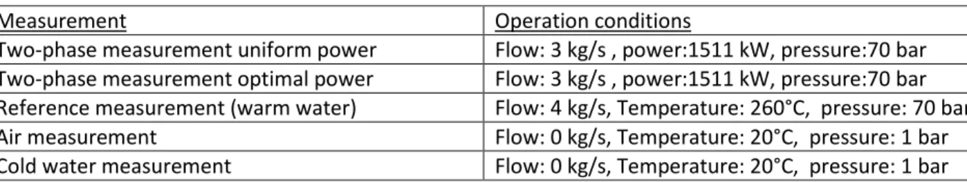
2.3 Measurement program

There were several different measurements done, both an average void measurement program with a few projections per height level designed to only measure the average void within the whole bundle, and detailed void measurements with more projections in order to get more detailed information about the void. The focus of this report is on the detailed void measurements done for fuel geometry with part length rods at three axial height levels called 𝑍= 1146 mm, 909 mm, 720 mm. This corresponds to 833 mm, 1070 mm and 1259 mm from the end of heated length (EHL) (above the part length rods). The beginning of heated length (BHL) is at 3740 mm from EHL. The two-phase measurements were done for two different radial power distributions, uniform power distribution and the optimal power distribution, as described in section 1.3. The main interest is in the fuel bundle which have part-length rods and how the void behaves above the part length rods. For each of the height levels five types detailed

tomographic measurements were done presented in Table 2-1. There was no flat field intensities measured because the object was not completely covered (chapter 2.3.1), but standard transmission measurements was done before and after each measurement (chapter 4.2.1).

Table 2-1 Five different types of measurement was done for each height level of interest (Z = 1146 mm, 909 mm and 720 mm).

The air and cold water measurements were done with no power or pressure pumps. The air measurement had cold water between the pressure vessel and the fuel bundle.

Measurement Operation conditions

Two-phase measurement uniform power Flow: 3 kg/s , power:1511 kW, pressure:70 bar Two-phase measurement optimal power Flow: 3 kg/s , power:1511 kW, pressure:70 bar Reference measurement (warm water) Flow: 4 kg/s, Temperature: 260°C, pressure: 70 bar

Air measurement Flow: 0 kg/s, Temperature: 20°C, pressure: 1 bar

Cold water measurement Flow: 0 kg/s, Temperature: 20°C, pressure: 1 bar

In the standard FRIGG setup, for all tests, several sensors for flow rates, pressure and temperature are placed inside the pressure vessel at different height locations. Some of data from these sensors was used to calculate the attenuation of water (chapter 4.1).

2.3.1 Measurement geometry

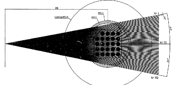
The detector board (Figure 2-1) was rotated around a center point in steps of ∆𝜃 = 1.34° for 153 projections. For each projection seven part-projections were done so that the detector elements is combined to 112 equidistant sensor positions (Figure 2-2), with detector element one corresponding to sensor position 1-7. In Table 2-2 a list of the number of projections and data measurement points is summarized. The exposure time for each part-projection was one second.

(11)

9

The fan-beam does not cover the range of the entire object for all projections and only the parts completely covered may be accurately reconstructed. The exterior object, i.e. outside the circle described by the rotating fan-beam cover, need to be compensated for either by mathematical description or by the use of references measurement (chapter 4.2.2).

Table 2-2 List of numbers of projections and combinations with part projections. The sensor position angular step is equal to the

part-projection angular interval.

Detector elements: 𝑘 16

Number of part-projections: 𝑞 7

Number of projections: 𝑝 153

Number of sensor positions: 𝑘 ∗ 𝑞 = 𝑟 112 Total number of projections: 𝑝 ∗ 𝑞 = 𝑙 1071 Total number of data points: 𝑝 ∗ 𝑟 = 𝑀 17136

Sensor positon angular step: ∆𝜑 0.2°

Projection angular step: ∆𝜃 1.3433°

3 Reconstruction Algorithms

3.1 Algebraic reconstruction

According to Beer’s law the transmitted intensities C can be expressed as 𝐶 = 𝐶0𝑒− ∫ 𝜇(𝑡)∙𝑑𝑡

Where C is the measured intensity (detector count), 𝐶0 is the intensity with no object present i.e. the flat

field intensity, µ(t) is the attenuation as a function of distance, t is the distance (position) from the source point. Rewritten for discrete form that becomes

3-1

Figure 2-2 The detector board and the measurement was moved to preform seven sub-projections so that the combined

coverage could be considered as a the above fan-beam geometry with sensor positions nr 1-112 in angular steps of 0.2° from 10.8° to -11.4° with sensor position nr 55 corresponding to the center beam. The fan-beam does not completely cover the pressure vessel or the isolation. In addition it does not cover the fuel bundle completely in some of the 153 projections. The distance from center of rotation to gamma source is 250 mm. Image courtesy of Westinghouse.

(12)

10 ln (𝐶𝑗

𝐶0) = − ∑ 𝜇(𝑡𝑖) 𝑁

𝑖=1 ∙ ∆𝑡𝑖,𝑗

where 𝑖 is the linear pixel index and 𝑗 is the sensor position. ∆𝑡𝑖,𝑗 is the distance a beam line travels

through a pixel. 3-2 can in turn be written in matrix form for a sought image where ∆𝑡 is called the weight matrix ( ln (𝐶1 𝐶0 ⁄ ) ln (𝐶2 𝐶₀ ⁄ ) ⋮ ln (𝐶𝑀 𝐶₀ ⁄ )) = − ( ∆𝑡₁₁ ⋯ ∆𝑡_1𝑁 ⋮ ⋱ ⋮ ∆𝑡𝑀1 ⋯ ∆𝑡𝑀𝑁 ) ( 𝜇₁ ⋮ 𝜇_𝑁)

M is the numbers of sensor positions in all projections, in this case M=17136. N is the total number of

pixels used to describe the area of interest. The weight-matrix describes the length each beam has to travel through each pixel and is calculated by a custom made weight-matrix algorithm developed by the authors of [5]. µ is the sought attenuation for each pixel in the region of interest and can be calculated from matrix division. In this work µ is solved by QR factorization [6].

3.2 Filtered back-projection

The Radon transform in two dimensions is the integral over a function along of a set of straight lines. The result is equivalent to the projections of absorption data measured in tomography. Then the inverse radon transform can be used to obtain an image of the object or function. The reconstruction algorithm is very efficient and since it operates in the frequency domain, a variety of frequency filters can easily be applied. Here, a Ramp-filter equivalent with the Hilbert transform is used. In this work the Matlab function iradon [6] was used which is a tool for the filtered back-projection method (FBP). 3.2.1 Interpolation to parallel beam geometry

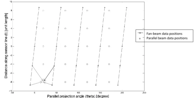
The tomographic measurement was done with a fan-beam geometry but the inverse radon transform requires a parallel beam geometry. Parallel beam data must then be constructed from the fan-beam data. The fan-beam geometry is a set of equally spaced data points in the 𝜃-𝜑 space to which each fan beam line has an exact corresponding parallel beam line in the 𝜃p-𝑑 space (Figure 3-1). From the fan

beam data points in the 𝜃p-𝑑 space, a set of parallel protection data can be calculated using linear

interpolation [7].

3-2

(13)

11

The resolution of a reconstruction using the inverse radon transform is limited by the linear spacing of the parallel sensor positions (∆𝑑). This has the consequence that in order not to ignore data points the spacing of 𝑑 must not be larger than the spacing between the fan-beam sensor positions in the 𝜃p-𝑑

space, ∆𝑑 < 𝑅 ∙ tan(∆𝜑). The same condition applies to ∆𝜃𝑝 that ∆𝜃𝑝< ∆𝜃, which holds for the chosen

values of ∆𝜃𝑝= 1.3°and ∆𝑑=0.8 mm.

4 Reconstruction and void calculation

Because of particularities of the test setup and the aim to achieve accurate void estimates, several adaptations of the reconstruction algorithms had to be implemented. Most noteworthy is the use of reference measurements. These are described in the subsections below.

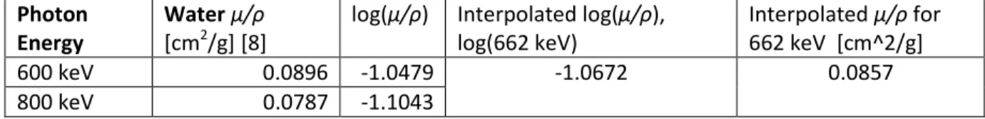
4.1 Calculating the attenuation of water at different temperatures

For each atom passed by the gamma on its track there is a specific probability for an interaction to take place. In macroscopic level this translates to values of a linear attenuation coefficient for specific elements. It is commonly given as the attenuation over density since the density of the particles is proportional to the attenuation. In [8] the values for water at two different energy levels are given. Since the attenuation can be approximated as a linear function in the log-log domain over the interval [8], interpolation is done over the logarithm values.

Figure 3-1 The fan-beams positions (*) in the 𝜽p-𝒅 space and a set parallel beam projections (o) to be

interpolated. The lines represent one fan-beam projection. The projections values for each parallel projection point can then be interpolated by linear interpolation from the four closest fan-beam projection points (arrows).

* Fan-beam data positions o Parallel beam data positions

(14)

12

Table 4-1 The interpolated data for the attenuation of the 662 keV gamma from Cs-137.

Photon Energy

Water µ/ρ [cm2/g] [8]

log(µ/ρ) Interpolated log(µ/ρ), log(662 keV)

Interpolated µ/ρ for 662 keV [cm^2/g]

600 keV 0.0896 -1.0479 -1.0672 0.0857

800 keV 0.0787 -1.1043

The density of water is given by its temperature and pressure. At the FRIGG loop, several temperature and pressure sensors give information about the conditions inside the pressure vessel. For each tomographic measurement, the temperatures and pressure were determined from the data given by these sensors. The temperatures at different levels were calculated by linear interpolation using temperature sensors above and below the fuel cross section of interest. In addition the attenuation for liquid water at the boiling point at 70 bar, 𝜇𝑙𝑏𝑝(70 𝑏𝑎𝑟) = 6.339 ∙ 10−3 mm-1, and for steam at 70 bar

𝜇𝑠(70 𝑏𝑎𝑟) = 0.313 ∙ 10−3 mm-1 is needed in order to transform attenuation maps to void maps

(chapter 4.3).

4.2 Problem specific adaptations and corrections

In order to accurately represent an object (without knowledge about its geometry), using standard tomographic reconstruction techniques, the object need to be completely covered by the fan-beam. As evident in Figure 2-2 the fan beam does not completely cover the object, therefore reference

measurements, which have identical geometry in the exterior of the covered object, are used. The reference measurements, with known geometry, are then used as corresponding flat-field intensities for each measurement point m. Since the exterior is the same in both cases the interior of the covered area can be reconstructed without artifacts induced by the exteriority of the covered object.

4.2.1 Correction for drifts in detector elements sensitivity

Before and after each measurement session a standard absorption measurement was done on a standard absorption slab. These measurements could be used to find the flat field intensities [9] however the available information of the slab dimensions and material composition was of inadequate accuracy. The standard absorption measurements are instead used only for measuring the relative detector efficiency changes between different measurements. This is done by taking the average of the standard absorption measurements done before and after each complete measurement session for each detector. The average is then used to create a factor used to correct for differences between each two-phase measurement and their corresponding reference measurement (4-1).

𝐶_𝑘,𝑙𝐷𝑉𝑐𝑜𝑟𝑟 ₌𝐶𝑘,𝑙𝐷𝑉∙𝑆𝑇𝐷𝑘𝑅𝐹 𝑆𝑇𝐷_𝑘𝐷𝑉

𝐶𝑘,𝑙𝐷𝑉 is the detector count for the detailed void measurement (two-phase measurement) for each

detector, 𝑘, and for every projection and part-projection, 𝑙. 𝑆𝑇𝐷𝑘𝑅𝐹 is the averaged standard intensity

count for the measurement used as reference for each detector, 𝑆𝑇𝐷𝑘𝐷𝑉 is the averaged standard

intensity count for the detailed void measurement. 𝐶_𝑘,𝑙𝐷𝑉𝑐𝑜𝑟𝑟 is the corrected detailed void measurement corrected for both changes in detector response and changes in source intensity between

measurements.

(15)

13

4.2.2 Specific corrections for algebraic reconstruction

The weight-matrix can only model the parts of the object that are inside the pixelated image. Some structures, such as the pressure vessel and the water outside the fuel bundle are outside of this

reconstructed image. Since the fan-beam does not cover the entire object the attenuation of the known structures outside the fuel mockup need to be modeled and corrected for.

Assuming that the isolation and the pressure vessel will give the same attenuation in both

measurements, reference measurement can be used to remove the influence of the non-beam-covered objects. Each measurement point then has its own corresponding flat field intensity, adapted from the reference measurement, and 3-3 then becomes

( ln (𝐶𝐷𝑉1 𝐶𝑅𝐹1 ⁄ ) ln (𝐶𝐷𝑉2 𝐶_𝑅𝐹2 ⁄ ) ⋮ ln (𝐶𝐷𝑉𝑀 𝐶𝑅𝐹𝑀 ⁄ ₎₎ = − ( ∆𝑡₁₁ ⋯ ∆𝑡_1𝑁 ⋮ ⋱ ⋮ ∆𝑡𝑀1 ⋯ ∆𝑡𝑀𝑁 ) ( 𝜇_𝐷𝑉1− 𝜇_𝑅𝐹1 ⋮ 𝜇_𝐷𝑉𝑁− 𝜇_𝑅𝐹𝑁)

where 𝐶𝐷𝑉𝑀 is the detector count for the detailed void measurement (two-phase flow) for sensor

position M and 𝐶𝑅𝐹𝑀 is the corresponding detector count in the reference measurement.

𝜇𝐷𝑉𝑁− 𝜇𝑅𝐹𝑁= ∆𝜇𝑁 is the calculated difference between the detailed void measurement and the

reference measurement for pixel N. 4-2 is equivalent to reconstructing the attenuation for each measurement separately then subtracting the attenuation images from each other. Furthermore, the assumption that the use of a reference measurement will eliminate the impact of the exterior is only valid when the outside conditions are similar between the measurements. That may be true for the pressure vessel and isolation, if the instrument and object relative positions are repeated, but it is not true for the water inside the vessel exterior of the image area. Here, differences in attenuation arise due to differences in temperature between measurements. To compensate for this, each beam’s path length through the water exterior of the image is calculated and the difference in attenuation between the outside liquid water subtracted. 4-2 then becomes

( ln (𝐶𝐷𝑉1 𝐶_𝑅𝐹1 ⁄ ) ln (𝐶𝐷𝑉2 𝐶_𝑅𝐹2 ⁄ ) ⋮ ln (𝐶𝐷𝑉𝑀 𝐶𝑅𝐹𝑀 ⁄ ₎₎ − ( ∆𝑡_𝑝𝑣1∙ (𝜇_𝑤_𝐷𝑉− 𝜇_𝑤_𝑅𝐹) ∆𝑡_𝑝𝑣2∙ (𝜇_𝑤_𝐷𝑉− 𝜇_𝑤_𝑅𝐹) ⋮ ∆𝑡_𝑝𝑣𝑀∙ (𝜇_𝑤_𝐷𝑉− 𝜇_𝑤_𝑅𝐹) ) = − ( ∆𝑡₁₁ ⋯ ∆𝑡_1𝑁 ⋮ ⋱ ⋮ ∆𝑡𝑀1 ⋯ ∆𝑡𝑀𝑁 ) ( 𝜇_𝐷𝑉1𝑐 _{− 𝜇} 𝑅𝐹1𝑐 ⋮ 𝜇_𝐷𝑉𝑁𝑐 _{− 𝜇} 𝑅𝐹𝑁𝑐 )

Where ∆𝑡_𝑝𝑣𝑀 is the distance through the water, exterior of the image area, for each beam path. 𝜇_𝑤𝐷𝑉− 𝜇_𝑤𝑅𝐹is the difference between the attenuation due to the difference in liquid water density between the reference measurement and the detailed void measurement, the pressure and

temperature is given by measured data from the Frigg loop and the corresponding density is then obtained from [10]. 𝜇𝐷𝑉𝑁𝑐 − 𝜇𝑅𝐹𝑁𝑐 =∆𝜇𝑁𝑐 is the corrected difference in attenuation for every pixel

described by the weight matrix as compared to the reference object.

4-3 4-2

(16)

14

4.2.3 Geometry corrections for the filtered back-projection method

The need to correct for differences in attenuation in the water exterior to the image area, as seen in chapter 4.2.2, is different for the filtered back-projection. The algorithm only reconstructs the image accurately within a circular area with the diameter equal to interpolated line source length, in this case ∅ = 𝑅 ∙ (tan(10.8°) + tan(11.4°)) = 98.1 mm. The exterior water is then in a virtual cylinder 3.6 mm thick from the inner radius of the presser vessel. Subsequently the correction is a small offset, applied to all projections, for each sensor position. As a consequence the correction is of less importance using the filtered back-projection method.

4.3 Calculating void image from attenuation image

The pixel void fraction is calculated from the difference in attenuation between the two-phase

measurement (mostly steam) and a reference measurement (water close to boiling point) as a fraction compared the attenuation difference between the attention of steam 𝜇𝑠 at 70 bar and the attention of

liquid water at boiling point 𝜇𝑙𝑏𝑝 at 70 bar. As in the case of the algebraic method, the water in the

reference measurement is below the boiling point. But the reference measurements were not made at the boiling point so the difference in liquid water attenuation between the two-phase measurement and the reference measurement has to be subtracted in order to calculate the void as the steam water fraction. The attenuation difference from the algebraic reconstruction (4-3) or from the iradon function

(chapter 3.2) is used in 4-4 to calculate the void

𝛼_𝑛=𝜇𝐷𝑉𝑛𝑐 −𝜇𝑅𝐹𝑛𝑐 −(𝜇𝑙𝑏𝑝−𝜇𝑤𝑅𝐹)

𝜇𝑠−𝜇𝑙𝑏𝑝 =

∆𝜇𝑛𝑐−(𝜇𝑙𝑏𝑝−𝜇_𝑤𝑅𝐹) 𝜇𝑠−𝜇𝑙𝑏𝑝

A consequence is that the rods are converted to the void domain even though there is no physical significance of the values in the rods. The expected void in the rods without correction for difference in water attenuation would have been zero, however the value is expected to be slightly negative since ∆𝜇 _𝑟𝑜𝑑 ≅ 0 and 𝜇𝑤𝐷𝑉< 𝜇𝑤𝑅𝐹.

5 Subchannel average void calculations

From the reconstructed images the subchannel void is calculated. The average void in a subchannel can provide validation data for subchannel analysis code, such as VIPRE-W. Different pixel patterns have been used for the subchannel averaging, as described in chapter 5.1.

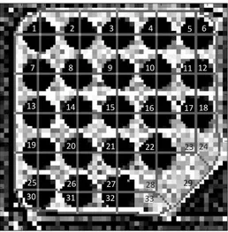
5.1 Subchannel geometry and pixel patterns

The subchannels are usually defined as the areas closed off by the shortest distances between four rod centers or wall boundaries (Figure 5-1). Also in the fuel geometries with missing rods in the examined axial level, due to part-length rods, the subchannel borders are based on the centers of the same rods, as if they were present. In order to calculate the subchannel average void three patterns to handle the rod pixels was devised. The first pattern uses a mask (chapter 5.2), the second pattern subtracts the

estimated influence from the rods on the average void (chapter 5.3) and the third pattern is a modified mask and subchannel boundaries (chapter 5.4, Figure 5-2).

(17)

15

5.2 Rod masking, pattern 1

The rods, visible in Figure 5-2, have no physical significance for the calculation of the void. Since the geometry of the rods is known to high accuracy a mask is used to separate the pixels in the rods and in the subchannels. However, due to the level of noise and various image artifacts in the rod positions, determining which pixels that are representing the rods is not trivial. The fact that the image is represented by square pixels and the rods are circular (Figure 7-7) further increases the difficulty in determining how to calculate the average void. In order to utilize the accuracy of the mask the image is up sampled by nearest neighbor interpolation. In effect the pixels are weighted by quarters determined by the location of the mask. The mask has a fixed geometry, i.e. the rods are not described

independently but as a bundle. Since the fuel bundles location in the image changes between height-levels the masks location in the image is determined by finding the lowest average value of the pixels covered by the mask.

5.3 Subtracting the rods influence, pattern 2

To avoid the problem of pinpointing the boundary of the circular rods in the rectangular pixel pattern, a second approach has been developed, where all pixels in a subchannel are used for calculating the subchannel average, including all pixels inside the fuel rod. Instead of masking these pixels, the influence of the known attenuation rod materials are accounted for. It can be noted that in the void domain, the use of reference objects should result in zero void inside the rod radius. However, some negative residual is caused by the lower temperature in the reference objects using liquid water. In addition, the rod positions are subject to statistical noise as well as rather strong edge-artifact, and possibly some objects are positioned slightly different from the corresponding reference object.

Figure 5-1 Pattern 1. A reconstructed image using the algebraic

methodwith the subchannels numbered and lined out. The rods have been masked to nearest quarter of a pixel. Black is zero void and white is 100% void. The subchannels are numbered from 1-33. The lower right corner is downstream the part-length rods and the neighboring subchannels are defined to were the centers of the part-length rods would have been.

Figure 5-2 Pattern 3. A reconstructed image using the algebraic

methodwith the subchannels lined out. The areas used to calculate the steam core subchannels is visible as the unaltered areas. The masking of the expected water film on the rods is visible as the darkened circles. The subchannels along the walls have been made smaller and the subchannels in the corners 1, 6 and 30 are removed. The part length rods are part of the mask for certain measurements.

10 20 30 40 50 60 70 80 90 10 20 30 40 50 60 70 80 90 1 2 3 4 5 6 7 8 9 10 0 11 12 13 14 15 16 6 17 18 / 19 20 21 22 23 24 / 25 26 27 28 29 30 31 32 33 6

(18)

16

Sinogram reference measurement Z=909 mm

sensor number (angle)

P ro je c ti o n n u m b e r (a n g le )

Sinogram Optimal/Reference STA corrected, Z=909 mm

Sinogram Optimal two-phase measurement STA corrected, Z=909 mm

5.4 Steam core average, pattern 3

In a stable two-phase flow water films are present on the surfaces of the rods and fuel bundle walls which lower the average void in a subchannel. To avoid the influence of water films the mask from pattern 1 was increased by 1.6 mm from all surfaces. In effect the rod mask radius was increased by 1.6 mm and the sub channels along the walls were diminished by 1.6 mm (Figure 5-2). In some cases the subchannels along the wall were removed completely as there were not enough pixels to calculate a trusted average. Furthermore with the larger mask, the effects of artefacts from rod misalignment and vibrations (chapter 8.2) are smaller as the affected pixels are ignored.

6 Validation of corrections

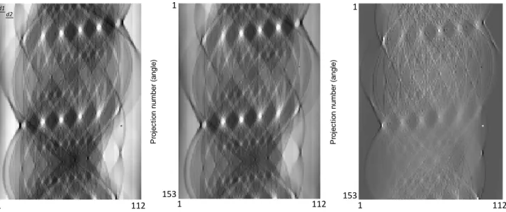
6.1 Result on sinogram of using reference measurement.

The data arranged by projection angle and sensor angle obtained from a tomographic measurement is called sinogram. By studying the sinograms of a reference measurement and a two-phase measurement and the sinogram obtained by dividing the values of the two-phase measurement and the reference measurement as in (4-2) one advantage of the use of reference measurement can be seen. In Figure 6-1 the data from each individual detector can be identified by intensity shifts for every seventh sensor position for the reference measurement and the two-phase measurement. But in the sinogram for the two-phase data divided by the reference data the detectors cannot be visually identified. By using reference measurements the problem with different detector responses and different flat field

intensities is easily resolved. Before this, the two-phase measurement has been corrected for detector variance in respect to the reference measurement in accordance to 4-1 (STA corrected).

Figure 6-1 Sinograms for measurements done at Z=909 mm. They are arranged by projection numbers (153) and sensor positions

(112) which can be converted to projection angle and sensor angle. The two-phase measurement for the optimal power distribution has been corrected using (4-1) for comparison with the reference measurement. The third image to the right is

calculated by dividing the intensity of each pixel in the two-phase measurement with the corresponding value in the reference measurement. Data from detectors one (d1) and two (d2) (sensor position 1-7 and 7-14) are marked in the reference

measurement. 1 1 153 112 1 1 153 112 1 1 153 112 d2 d1 R

(19)

17

7 Results

The two methods were used to reconstruct and calculate the pixel void for three axial positions (z = 1146 mm, 909 mm and 720 mm) for each of the two radial power distributions. Some example results are presented in chapter 7.1 and 7.2, for all images see Appendix A: Two phase reconstruction and Appendix B: Reconstructions of Air to Water measurements.

7.1 Results of the algebraic reconstruction method

The algebraic method was used to make reconstructions with two different resolutions. The pixel sizes used were 1.5 mm and 1.25 mm which resulted in images of 49x49 pixels and 59*59 pixels. The pixel size 1.5 mm was chosen as primary resolution in accordance to [9]. At the 720 level, the part length rods are visible (Figure 7-4 and Figure 7-3). They have a different constitution than the other rods with a second heating element looping back through the rod.

Figure 7-1 Image of the void distribution for

two-phase flow with the uniform power distribution at Z= 909 mm and 1.5 mm pixels. Void α=1 is white and α=0 is black.

two-phase flow with the uniform power distribution at Z= 909 mm and 1.25 mm pixels. Void α=1 is white and α=0 is black.

two-phase flow with the optimal power distribution at Z= 720 mm and 1.5 mm pixels. Void α=1 is white and α=0 is black.

two-phase flow with the uniform power distribution at Z= 720 mm and with pixel size 1.5 mm. Void α=1 is white and α=0 is black.

(20)

18

There is no obvious difference between the optimal and uniform measurements evident by looking at Figure 7-4 and Figure 7-3, but by calculating the subchannel void distribution a difference can be inferred, see chapter 7.4. The noise level is apparently large, with several pixels having unphysical void levels below zero or higher than that of saturated steam. This noise is larger in the reconstructions with higher resolution, which can be expected since the more pixels used, the lower is the number of

measured constraints per unknown variable. The part length rods are ending at the 720 level and there is a difference in the interior of the rods between the reference measurements and the two phase

measurements, which can be explained by the rods ending on just slightly different heights between measurements.

7.2 Filtered back-projection

The filtered back-projection method does not have any constraints on the number of pixels used, in the sense that the algebraic method has. Instead there is an upper limit for the pixel size which is 0.8 mm as explained in chapter 3.2.1

The resolution in Figure 7-5 and Figure 7-6 is higher without the apparent increase in noise levels, which the algebraic method is subject to. But in several locations there seems to be higher void at the upper right side of each rod. This issue is discussed further in chapter 7.3 and chapter 8.

7.3 Comparison with air to water reference measurements

The two-phase measurements and the reference measurements were done with high pressure and high heat flux, and the resulting images have higher noise levels than the cold measurements. The noise levels make it difficult to evaluate the effectiveness of the different methods. The conditions during the cold water measurement and air measurement were more stable, with no applied pressure and no heating. These measurements have been used to compare the quality of each method. In order to compare the results, the reconstructed values of the attenuation are rescaled to the void domain in accordance to 4-4. Because the air and water measurements have no differences in attenuation in the exterior water area and air can be interpreted as steam 4-4 becomes 7-1.

Figure 7-6Pixel void for the optimal power distribution at z=1146 mm. Void α=1 is white and α=0 is black. Pixel size is 0.8 mm.

Figure 7-5 Pixel void for the optimal power

distribution at z=909 mm. Void α=1 is white and

(21)

19 𝛼_𝑎= ∆𝜇̅𝑎

𝜇𝑎𝑖𝑟− 𝜇𝑤

∆𝜇̅_𝑎 is the calculated attenuation difference for each pixel between the cold water measurement and air measurement ,the latter is seen as a two phase measurement. 𝜇𝑎𝑖𝑟 is the attenuation of air which is

assumed to be zero, 𝜇𝑤 is the attenuation of cold, liquid water, calculated as 0.00855 mm-1 (chapter 4.1).

For the algebraic method several pixel sizes was investigated and visible artifacts, especially in the middle, are present for pixels size smaller than 1.25 mm (Figure 7-8). The reconstructed image with pixel size 1.5 (Figure 7-7) has less such artefacts and is a much clearer image compared to two-phase

measurements. In the images with lower resolution effects of spatial aliasing (chapter 5.2) is evident as grey pixels in the boundary between rods and subchannel. For full list of images see Appendix B.

In chapter 3.2.1 an upper limit of the pixel size for the filtered back-projection method is determined to be 0.8 mm. Compared to the lower limit of 1 mm pixels size for the algebraic method the filtered back-projection method has higher resolution than the algebraic method as applied here. But inspection of Figure 7-9 shows a pattern of lighter and darker patches that is arranged in horizontal stripes. The rods

Figure 7-7 Same conditions as Figure 7-8 but with 1.5 mm

pixels. Spatial aliasing is evident as there are grey pixels in the rods circumference.

Figure 7-9 FBP reconstructed image for air with cold

water reference measurements. Axial level is 1146 mm and the pixel size is 0.8 mm.

7-1

Figure 7-8 Difference between air and water measurement

done with the algebraic method. Z=1146 mm and pixel size is 1 mm. The black line is not believed to be an artefact from the reconstruction but rather a discrepancy of the detector response in this specific measurement.

(22)

20

Figure 7-10 the calculated subchannel void distribution with the rods masked for the void image calculated with the algebraic method,

optimal power distribution at z=909 mm and with pixel size 1.5 mm. A: Pattern 1, the subchannel void calculated with the rod-pixels omitted. B: Pattern 2, the subchannel void calculated for all pixels in a subchannel with the contribution of the rods subtracted. The rods are visually marked. C: Pattern 3, the average void for the sub channel steam core. D: The average void image with the rods masked. For A,B and C their corresponding total average is given in the table in the middle.

also appear slightly distorted because of the gradients in the image between light and dark areas. The rods appear to shadow some places and increase the pixel values in others. Such artefacts are typical when using the filtered back-projection method as it performs poorly when sharp edges are present in the object [11]. That is the case with the boundaries between rods and subchannels. Due to the artefacts the algebraic method was chosen over the filtered back-projection method, see chapter 8.1

7.4 Presentations of average subchannel void

The average subchannel void was calculated using three methods described in chapter 5. For each method an average of all subchannel average void was calculated from the void in each subchannel weighted with its area.

In Figure 7-10 subchannel void in the corner seems to be slight lower than the void in the rest of the subchannels. The void in the steam core (C) is higher than the void calculated for the whole subchannel, due to the fact that water films are present on the surface on the rods. The subchannels along the walls have a higher void but there are too few pixels to have statistical accuracy of the values in those pixels (chapter 7.4.1). Furthermore the walls might be slightly misaligned between measurements and then a large number of pixels in the wall subchannels will have a misleading value.

A B D _α _C α α α α

0.76

0.74

0.80

(23)

21 7.4.1 Noise estimation

As seen in chapter 7.1 and chapter 7.3 there is more noise in the two-phase measurements compared to the air-water measurements. That might be because of misalignment and high steam flow in the two-phase measurement, see chapter 8.2. A way to quantify the effect of the noise on the subchannel void estimates is to calculate the standard error of mean (7-1).

𝜎

√𝑁= 𝜎mean,

where N is the number of pixels. Due to the presence of duplicate pixel values from the mask adjustments (chapter 5.2) the standard deviation was calculated for each unique pixel value in the subchannel. Furthermore in order to use this method other assumptions regarding correlations between pixels have been made which is discussed in chapter 8.3.

In Figure 7-11 it can be seen that the statistical noise for the subchannels along the walls is higher and the value therefore more uncertain. The uncertainty is the least for the large subchannel in the lower right corner. In case C the number of pixels used to calculate the average was fewer when compared to case A and B so the uncertainty is higher. In case B, where more pixels are used to calculate the

subchannel average, the standard error of mean is lower than in the other cases, despite the fact that there is a larger variation in pixel values between rod pixels and channel pixels. The average error is around 0.09 void units for case B compared to 0.12 void units for case C and 0.11 void units for case A.

7-1

Figure 7-11 Maps over the standard error of mean corresponding to A,B and C in Figure 7-10. The color scale was chosen to

highlight differences between sub channels along the walls and the subchannels in the middle of the subchannel. Some values are much higher than the range of the color scale.

A C B Vo id u n its Vo id u n its Vo id u n its

(24)

22

Figure 7-12 Comparison with VIPRE-W simulations, for z=909 mm and optimal power distribution. The relative power between

rods is show in greyscale with light indicating higher power and grey indicating lower power. Total void is the subchannel void calculated with the rods masked (Pattern 1). The steam void is calculated as the subchannel steam core values (Pattern 3). Corner values with rods were omitted.

7.5 Comparison with VIPRE-W calculations

VIPRE-W is a program that calculates the avarage subchannel void given input of pressure, flow rate, power and power distribution. A comparison with the tomographic reconstruction was done for two resolutions of the algebraic reconstruction (Figure 7-12).

The VIPRE-W simulations show a slightly lower void in the corner with no rods, which is also what the tomographic measurements show. The measurements show that the void is about 7 % void percent units lower in the part length subchannel which is about 8 % lower than the center subchannels for the total void. In comparison the standard error of mean are about 10 % void percent units but only about 3 % void percent units for subchannel 29. However the standard error of mean is not an accurate method for determining the error, see chapter 8.3. But due to the variance of subchannel void reconstructions it is difficult to draw conclusions other than that there seems to be no large deviation from the predictions of the VIPRE-W simulations. The filtered back-projection method show a relative larger difference between total void (including water film) and the steam core void.

8 Discussion

8.1 Selection of reconstruction algorithm

The filtered back-projection method has a better spatial resolution than the algebraic method, however the artefacts from the transform is evident in Figure 7-9. The white and gray shadowing effects do not affect the geometric shape of the object, but the void in each pixel and subchannel becomes difficult to assess. This becomes evident in when studying the FBP case in Figure 7-12. The void along the left side wall and lower side wall for the total void is lower than the void in the other subchannels when in the algebraic method the opposite is true. When looking at the average void for all subchannels the filtered

Algebraic, 1.25 mm Algebraic, 1.5 mm VIPRE-W To tal v o id Steam c o re

(25)

23

back-projection method results in lower values of void which does not agree with the expected total average void. The algebraic method does not have such artefacts and for calculating the average subchannel void that is more important than spatial resolution. However the algebraic method is sensitive to noise in the data as errors in one point might affect the solution of several other points.

8.2 Misalignment between two-phase and reference measurements

When comparing images of two-phase void with the air-water images the difference in quality of the description of the rod is clear (Figure 7-1 and Figure 7-8). An explanation for this is that the fuel bundle might have been removed and inserted again since there were different fuel geometries and

measurements were done on different days. In Figure 7-2 along the left wall there is a row of high void pixels with a row of very low void pixels right left of it. This implies that the left wall between

measurement have moved slightly resulting in attenuation differences that result in high-low void structures. Furthermore the flow, pressure, and heat expansion could have made the rods move relative to each other and the walls. Part of the structures visible inside the rods (see Figure 7-2 ) can also be explained by this as the inner structure of the rods is that of two cylinders of high attenuation metal material with low attenuation isolation material between. However the misalignment between

measurements is expected to be small in the scale of < 1 mm. The steam core average void can then be considered to be more accurate than the complete subchannel void, considering the possible

displacement of the rods, as the steam core values are based on pixels is located 1.6 mm and more from all high-attenuation structures.

8.2.1 Vibrations in the rods

In the phase measurement the rods are heated which cause expansion of the material. The two-phase flow is also varied especially with height level. At some levels there is slug flow with high variation in density. These variations in the flow and expansion cause the rods to vibrate which would be seen as circular artifacts in the rods and slightly higher void around the circumference of the rods. In chapter 7.1 the noise in the rod seems to be like circular artefacts and around some rods a small area of higher void can be seen, often in the upper-right hand side of rods.

8.2.2 Use of image alignment software

The reconstruction is a linear operation which means that there is no mathematical difference in dividing the intensities 𝐶𝐷𝑉𝑀 and 𝐶𝑅𝐹𝑀 before the reconstruction or subtracting two separately reconstructed

images from the same measurement data. There is however ever a difference in computation time which is doubled because two reconstructions are done rather than one. As mentioned in chapter 8.2 the fuel bundles can be misaligned, which causes errors in calculating the void. By reconstructing the reference measurement and the two-phase measurement separately, prior to subtraction to achieve the void image, image processing might be used to align the rod structures and improve the results.

However there is difficulties to this method as the misalignment is often less than the pixel size (<1 mm) used in representing the image, in addition the individual pixels have a substantial level of noise. Then a new image has to be interpolated in order to move the structure a smaller distance in the image than the pixel size. The development of a suitable image processing algorithm may also prove challenging. Tests using matlab function imregister have been used for preliminary tests of such an approach, but it was not found

to improve the void images in a satisfactory way.

8.3 Noise estimation of the average subchannel void

To estimate the noise level and to estimate the accuracy of the method the standard error of the mean was calculated (7-1) for each subchannel. But the standard deviation is not a very good method because of several not so obvious assumptions that has to be made. The first assumption is that the values are

(26)

24

uncorrelated, which is an underlying assumption when using the standard error of the mean. This is however not true for the pixels of a tomographic reconstruction. The measurements are of the average attention for a beam path which in combination with the other projections gives the reconstructed image. In the solution, however, a pixel can then be solved for a value higher than it actually is and then the neighboring pixel, as compensation, is solved as a lower value. That implies that neighbor pixels may have negative correlation coefficients.

Furthermore, the standard error of the mean is based on the assumption that the pixel values are sampled stochastic variables of the same population, i.e., the same probability distribution and the same true average and variance. This is likewise not true, since large variations of the void are to be expected within the subchannels. For example, at high axial locations in the fuel, such as above the part-length rods, the flow type is predominantly annular flow, where the void fraction is very low close to the fuel rod, where a liquid film is present, and the void fraction is much higher in the central subchannel. Therefore, the usage the standard error of the mean is at best a rough estimate of the uncertainty of the measurement results. Finally, because of the method for fitting the mask described in chapter Rod masking5.2 the standard deviation is calculated for all pixels not completely covered by the mask which is slightly larger area then for the subchannels average.

8.3.1 Evaluating the different reconstruction methods

There has been no quantified comparison between the reconstruction methods but as discussed in chapter 8.1. the filtered back-projection method has artefacts not necessarily reveled by calculating the standard deviation. Determining the optimal resolution for the algebraic method using this method is also not obvious as the difference between pixels values might come from actual difference in

attenuation instead of noise. One measure might be to calculate the standard deviation for the pixels in the rods which should be closer to zero but as discussed in chapter 8.2 the difference might not come from inaccuracy in the calculation method but from misalignment. In [9] the a resolution close to 50x50 pixels where chosen so the 1.5 mm can be consider as the primary calculation method.

9 Conclusions

Two methods, one algebraic and one filtered back-projection method, for tomographic reconstruction were implemented and a comparison between them was done using low noise calibration

measurements. The algebraic method was found to be the more suitable of the two for the tomographic measurements done at FRIGG. The filtered back-projection method was found unsuitable for the

reconstruction of detailed void measurements due to the artefacts from high differences in attenuation in the object (chapter 7.3 and 8.1). The detailed void measurement done downstream the end of the part length rods was reconstructed and the subchannel average void was calculated. Three methods for calculating the subchannel average void was compared with computer simulation code. The measured subchannel average void shows a reasonable agreement with predictions and simulations (chapter 7.5). The void in the region downstream the part length rods is found to be slightly lower, about 1%, than the void in the other subchannels (chapter 7).

10 Outlook

The images are quite coarse and some are quite noisy. There are other methods of solving an over determined linear equation system, but there are also issues inherent with the measurements which could be improved. A more precise mathematical description of beam paths modelling the cross section of the source and the cross sections of the detectors could be implemented. More complex iterative solving algorithms, that could be less noise sensitive at higher resolution, are a possibility for improving

(27)

25

the result. For example adding constraints of physical values of attenuation to the solution or make other parameterizations than square pixels. Estimations of the errors can be done using synthetic data and such error simulations can be used to find the largest error contributions.

A short attempt was done in applying an image alignment method but was abandoned as the result of the reconstructions was not improving enough to warrant the time. However with more time and more sophisticated tools and knowledge it is likely to improve the results.

The exposure time for each measurement with a detector was one second which might not have been long enough to accurately form an average over the changing two-phase flow. The exposure time should be long enough so that the expected fluctuations in the attenuation due to shifting void are on the level of the statistical error of the detector, which is about 0.15 %. The effects of two-phase fluctuations can be simulated and with time discrete transmission data for a sight line a suitable measurement time for the projections can be found. The measurement time should so that both the statistical error in the detectors and the two-phase fluctuations converge [12].

11 References

[1] Statistiska Centralbyrån, "SCB," Statistiska Centralbyrån, 17 12 2013. [Online]. Available: http://www.scb.se/sv_/Hitta-statistik/Statistik-efter-amne/Energi/Tillforsel-och-anvandning-av-energi/Arlig-energistatistik-el-gas-och-fjarrvarme/6314/6321/24270/. [Accessed 25 11 2014]. [2] J.-M. Le Corre, C. Adamsson and Brynjell-Rahkola, "Validation of VIPRE-W Sub-channel Void

Predictions," in NURETH-13, N13P1080, Kanazawa, 2009.

[3] O. Nylund, Upgrade of the FRIGG test loop for BWR fuel assemblies, Västerås: ABB Atom AB, 1997. [4] G. Windecker and H. Anglart, "Phase distribution in BWR fuel assembly and evaluation of

multidimensional multi-field model," in NURETH-9, San Fransisco, California, October 3-8 1999. [5] P. Andersson, S. Jacobsson Svärd, E. Andersson Sundén and H. Sjöstrand, "Neutron tomography of

axially symmetric objects using 14 MeV neutrons from a portable neutron generator," REVIEW OF

SCIENTIFIC INSTRUMENTS, vol. 85, 2014.

[6] The MathWorks, Inc., "Matlab Documentation," 2014. [Online]. Available: http://se.mathworks.com/help/.

[7] P. Andersson, T. Bjelkenstedt, E. A. Sundén, H. Sjöstrand and S. Jacobsson-Svärd, "Neutron tomography using mobile neutron generators for assessment of void distributions in thermal hydraulic test loops," submitted to Physics Procedia, 2014.

[8] Pysical Measurement Laboratory, "Tables of X-Ray Mass Attenuation Coefficients," The National Institute of Standards and Technology, 08 10 2014. [Online]. Available:

http://physics.nist.gov/PhysRefData/XrayMassCoef/tab4.html. [Accessed 10 09 2014].

[9] K. Holmquist, "Tomograpic reconstruction of the void distrution in the nuclear fuel test loop FRIGG," Uppsala Univetsity, Uppsala, 2006.

[10] Spirax Sarco, "Steam Tables," Spirax Sarco, 2015. [Online]. Available:

http://spiraxsarco.com/resources/steam-tables.asp. [Accessed 11 11 2014].

[11] F. E. Boas and D. Fleischmann, "CT artifacts: Causes and reduction techniques," Imaging Med., vol. 4, no. 2, pp. 229-240 , 2012.

[12] P. Andersson, E. Andersson Sundén, S. Jacobsson Svärd and H. Sjöstrand, "Correction for dynamic bias error in transmission measurements," REVIEW OF SCIENTIFIC INSTRUMENTS, no. 83, 2012.

(28)

Appendix-A: Two-phase reconstruction

FBP, Optimal, Z 909 mm, 0.8 mm pixels FBP, Optimal, Z 1146 mm, 0.8 mm pixels

FBP, Uniform, Z 909 mm, 0.8 mm pixels FBP, Uniform, Z 1146 mm, 0.8 mm pixels

Algebraic, Optimal, Z 720 mm, 1.25 mm pixels Algebraic, Optimal, Z 909 mm, 1.25 mm pixels

(29)

Algebraic, Optimal, Z 1146 mm, 1.25 mm pixels Algebraic, Uniform, Z 720 mm, 1.25 mm pixels

Algebraic, Uniform, Z 909 mm, 1.25 mm pixels Algebraic, Uniform, Z 1146 mm, 1.25 mm pixels

Algebraic, Optimal, Z 720 mm, 1.5 mm pixels Algebraic, Optimal, Z 909 mm, 1.5 mm pixels

(30)

Explanation of titles:

Reconstruction method (Algebraic/FBP), Power distribution (Optimal/uniform), axial level (z [mm]), pixel size ([mm])

Algebraic, Optimal, Z 1146 mm, 1.5 mm pixels

Algebraic, Optimal, Z 909 mm, 1.5 mm pixels Algebraic, Uniform, Z 720 mm, 1.5 mm pixels

Algebraic, Uniform, Z 909 mm, 1.5 mm pixels Algebraic, Uniform, Z 1146 mm, 1.5 mm pixels

(31)

Appendix B: Reconstructions of Air to Water measurements

FBP, Z 1146, 0.3 mm pixels FBP, Z 1146, 0.6 mm pixels

FBP, Z 1146, 0.8 mm pixels FBP, Z 1146, 1.0 mm pixels

FBP, Z 1146, 1.5 mm pixels Algebraic, Z 1146, 0.8 mm pixels

(32)

Iterativ_Water_Air_Z720_ims73.5_pxS1.5_iterativRekonWater.mat 5 10 15 20 25 30 35 40 45 5 10 15 20 25 30 35 40 45

Iterativ_Water_Air_Z909_ims73.5_pxS1.5_iterativRekonWater.mat

5 10 15 20 25 30 35 40 45 5 10 15 20 25 30 35 40 45

Explanation of the titles:

Reconstruction method (Algebraic/FBP), axial level (z [mm]), pixel size ([mm])

Algebraic, Z 1146, 1.0 mm pixels Algebraic, Z 1146, 1.25 mm pixels