Method
An Analysis of Willingness to Pay to Reduce Mortality Risk
Henrik Andersson1,?, Mikael Svensson21 Dept. of Transport Economics, Swedish National Road and Transport Research Institute (VTI), Sweden 2 Dept. of Business, Economics, Statistics & Informatics, ¨Orebro University, Sweden
February 12, 2007
Abstract This study investigates whether or not the scale bias found in contingent valuation (CVM) studies on mortality risk reductions is a result of cognitive constraints among respondents. Scale bias refers to insensitivity and non near-proportionality of the respondents’ willingness to pay (WTP) to the size of the risk reduction. Two hundred Swedish students participated in an experiment where their cognitive ability was tested before they took part in a CVM-study where they were asked about their WTP to reduce bus-mortality risk. The results imply that WTP answers from respondents with a higher cognitive ability are less flawed by scale bias.
Key words cognitive ability; contingent valuation; mortality risk; near-proportionality; scale bias JEL codes: D80; I10; Q51
? To whom correspondence should be addressed. Corresponding address:
1 Introduction
Economists usually prefer revealed-preference (RP) to stated-preference (SP) methods when non-marketed amenities are to be evaluated. Preferences in RP-studies are not only based on actual choices made by individuals, but it is also assumed that actual choices, compared to hypothetical choices made by re-spondents in SP-studies, are made on a more informed basis. SP-methods have an important role to play when knowledge among analysts about the decision alternatives and the consequences decision makers face is limited, or when market data does not exist for the amenity of interest. One SP-method that has been used to evaluate a wide range of non-marketed amenities is the contingent valuation method (CVM), a method where respondents are asked directly about their willingness to pay (WTP) for the amenity.
CVM has been under heavy criticism for being inadequate to measure individual preferences (Dia-mond and Hausman, 1994). In addition to the criticism of hypothetical bias, much of the criticism has been based on the lack of scale sensitivity found in many CVM-studies.1This has particulary been found in studies on “non-use values”, where respondents have been found to be willing to pay the same amount to save wild species or protect environmental resources regardless of numbers and amounts (Desvousges et al., 1993; Kahneman and Knetsch, 1992). Whereas the advocates of CVM consider the lack of scale sensitivity to be a result of bad survey design (Carson and Mitchell, 1995; Carson et al., 2001; Smith, 1992), its opponents argue that it is not capable of eliciting individual preferences (Desvousges et al., 1993; Diamond and Hausman, 1994; Kahneman et al., 1999). Recent research suggests, however, that a general dismissal of the CVM on the basis of scale insensitivity is unwarranted, and that scale insen-sitivity can be in line with economic theory, and may also appear in well conducted studies (Heberlein et al., 2005). For instance, if respondents prefer to save 300 rather than 800 wolves (Heberlein et al., 2005, p. 16), a standard scale test in a CVM-study would falsely reject the WTP answers as not being valid estimates of the respondents’ preferences.
When individuals’ preferences for a reduction of their own mortality risk are elicited, respondents of CVM-studies are usually asked to state their WTP for small reductions in the probability of death. Since individuals will personally benefit from the risk reduction, we expect them to be willing to pay more for a larger risk reduction than for a smaller one. Hence, scale sensitivity is here a necessary condition for the estimates to be valid. Moreover, WTP should also be near-proportional to the size of the risk reduction (Hammitt, 2000a). Eliciting individuals’ preferences for reductions in the probability of death seems, however, to be cognitively constraining for the respondents (Carson et al., 2001). Hammitt and Graham (1999) analyzed scale sensitivity in 25 CVM-studies on mortality risk reductions, and found that WTP increased with the size of the risk reduction in most of them. In none of the studies was the
increase in WTP near-proportional to the risk reduction. In addition, Hammitt and Graham (1999) also performed a scale sensitivity test on their own data set in the study. Different samples answered questions on risk reductions of different size, with the large risk reduction being 10 times greater than the smaller one. Among other things they tested if it had any effect on the analysis of scale sensitivity to include only individuals who answered correctly to a single question regarding probability comprehension. They found no such effect. What they did find however, was that respondents with higher confidence in their answers, gave answers with close resemblance to theoretical predictions. This is in line with the results in Corso et al. (2001) and Alberini et al. (2004) where proportionality could not be rejected for “better informed” and “more confident about their answers” respondents, respectively.
Psychology literature has shown that we often make decisions based on heuristics (short cuts), since mental short cuts lighten the cognitive burden of decision-making (Kahneman et al., 1982; Kahneman, 2003). Cognitive constraints, it is argued, make the kind of questions employed in SP-studies impossible to implement with accuracy. In this study we investigate whether or not cognitive constraints can explain the lack of scale sensitivity found in CVM-studies on mortality risk reductions. We assume that individuals with lower cognitive ability have a higher share of decision-making driven by heuristics, which results in less well-considered answers. Our hypothesis is that respondents with a higher cognitive ability are more able to understand the probability changes and, therefore, state a WTP that is more proportional to the magnitude of the risk reduction and thus more in line with the theoretical predictions. The aim here is to test this hypothesis, and we do this by letting a sample of Swedish students take part in an experiment where, prior to answering WTP questions, they take part in a test, the result of which is used as a proxy for cognitive ability. Thus, we examine whether or not cognitive ability is correlated with WTP answers in line with our hypothesis. In the survey the students are asked about their WTP to reduce the mortality risk they face when riding the local bus, a risk we assume most respondents are familiar with.
The paper is structured as follows. The following section contains the theoretical model and a discus-sion on why WTP should be near-proportional to the magnitude of the risk reduction. The experiment is described in section 3. The data that was collected and the regression results in section 4 reveal a positive correlation between cognitive ability and WTP answers less flawed by scale bias. This is especially true for respondents with the highest score in the test of cognitive ability and for respondents with good skills in probability laws, compared with respondents only showing good skills in pure computational exercises. Finally, the last section offers a discussion and some concluding remarks. Our findings con-firm that knowledge and understanding of the good in CVM-studies are important in order to get valid
WTP estimates. Part of the scale insensitivity found in CVM-studies can, therefore, be regarded as a methodological problem, and hence a problem which can be reduced with more research.
2 Marginal Willingness to Pay to Reduce Mortality Risk
The population mean of marginal WTP to reduce mortality risk is usually denoted “the value of a statistical life” (VSL), and is a measure of the marginal rate of substitution between mortality risk and wealth. The decision individuals face can be illustrated with a state-dependent expected utility model (Rosen, 1988). Let w, p, and us(w), s ∈ {a, d}, denote wealth, baseline probability of death, and the
state-dependent utilities, respectively, with subscripts a and d denoting survival and death. The survival lottery will then be given by
EU0(w, p) = pud(w) + (1 − p)ua(w). (1)
For a marginal change of p we have the standard result that
VSL = dw dp ¯ ¯ ¯ ¯ EU constant = ua(w) − ud(w) pu0 d(w) + (1 − p)u0a(w) , (2)
where prime denotes first derivative (Hammitt, 2000b). Under the reasonable assumptions (which are standard in the literature) that ua(w) > ud(w), u0a(w) > u0d(w) ≥ 0, and u00s(w) ≤ 0 for s ∈ {a, d}, VSL
is positive and increasing with w and p (Jones-Lee, 1974; Weinstein et al., 1980).2
Equation (2) denotes “true” marginal WTP. In CVM-studies respondents are asked to state their WTP for a small but finite risk reduction, ∆p. Now let w0 and p0 denote the initial wealth level and baseline risk in equation (1). WTP in equation (3) then defines the maximum amount an individual is willing to pay to reduce, remaining at the same utility level, the mortality risk by ∆p, i.e.
EU1= (p0− ∆p)ud(w0− WTP) + (1 − p0+ ∆p)ua(w0− WTP) = EU0. (3)
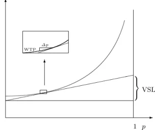
WTP will be increasing and concave with ∆p. Moreover, as mentioned, a necessary (but not suffi-cient) condition for WTP answers from CVM-studies to be valid estimates of individuals’ preferences for mortality risk reductions are that they are near-proportional to the size of ∆p (Hammitt, 2000a). Equation (2) can be used to illustrate the effect of ∆p on VSL, which will be less than or equal to 1/[1 + ∆p/(1 − p)].3 The income effect on VSL is not constrained by the theoretical model. Empirical evidence suggests that the income elasticity of VSL is less than one, and based on that evidence Ham-mitt (2000a) showed that the income effect would only cause a small departure from proportionality. The relationship between marginal and non-marginal WTP is also illustrated in Figure 1. For small p,
the distance between the tangent to the indifference curve at the initial baseline risk and the indifference curve, after the risk reduction, will be small, and hence WTP is near-proportional.
[Figure 1 about here.]
Let us also illustrate the near-proportionality with a numerical example. We employ the state-dependent utilities from Pratt and Zeckhauser (1996), i.e. ud(w) = ln(w) and ua(w) = 10 + 5 ln(w),
and we let w, p, and ∆p be given, and estimate WTP. Two different scenarios are included, one with a higher baseline risk and one with a lower risk. In each scenario WTP is estimated for two different risk reductions. The ratio between these risk reductions is 2.5 in both scenarios. The purpose of this setup is to show that the departure from proportionality is smaller for the low p and small ∆p, but near-proportional also for the high p and larger ∆p. As can be seen in Table 1, the WTP ratio in the “low risk” scenario is closer to proportionality than the WTP ratio in the “high risk” scenario, 2.498 and 2.453, respectively. The baseline risk in the “high risk” scenario has been deliberately chosen to be relatively high for a mortality risk, ph= 0.01, and since the percentage risk reductions are equal in the
high and low risk scenarios, this consequently means that the risk reductions also are relatively large. Still, WTP is near-proportional for these risk reductions as well.
[Table 1 about here.]
3 The Experiment
The experiment was conducted on 200 undergraduate students at Karlstad University in Sweden in the fall of 2005.4The students were informed in class that they would be given the opportunity to take part in an experiment with the aim of providing valuable information for government authorities within the transport sector. They were not informed that the aim was to examine how WTP is affected by cognitive skills, since we suspected that it could increase the number of protest answers. The students were informed that the experiment would take place after the next lecture of the class, that participation would be voluntary, and that they would receive SEK 50 (ca. USD 7) as compensation for their participation.5 In order to avoid “interviewer bias” the same person: (i) informed the students about the opportunity to take part in the experiment in class, and (ii) was present during the experiment, handing out the questionnaires to the students and informing them about how the experiment was going to be carried out.6
The experiment consisted of three parts: (i) the test of cognitive ability, (ii) the CVM-survey, and (iii) follow-up questions on demographics, socio-economics and some questions related to academics and “traffic experience”. The test of cognitive ability and an alternative variable to measure cognitive skills are contained in the next section, followed by a section where the CVM-survey is briefly described.7
3.1 Cognitive Ability
In the cognitive ability test the respondents were given 5 minutes to answer 17 questions. A pilot study, conducted prior to the main study, contained 15 questions. In view of the low variance of the test score in the pilot study, we decided to add 2 questions to the main study. The test is not in any way a complete cognitive ability test, instead we focus on the respondents’ skills in thinking about probabilities, syllogisms and computation; which have been deemed important in related studies (Benjamin and Shapiro, 2005).8 Recent research has shown, however, that simple tests with only a few questions can work as well as longer tests, such as the Wonderlic or SAT tests, to measure cognitive ability (Frederick, 2005).9
Cognitive processes are by many distinguished into two types of processes (Epstein, 1994; Kahne-man and Frederick, 2002; SloKahne-man, 1996). Stanovich and West (2000) label these processes System 1 and 2 and they can be described as “automatic, largely unconscious, and relatively undemanding of computational capacity” and “conjoins the various characteristics that have been viewed as typifying controlled processing”, respectively (Stanovich and West, 2000, p. 658).10 Hence, System 2 is the cogni-tive processes operating when we use formal rules and concentration, in opposite to the instant reaction process of System 1. For instance, consider the following question, which was included in our cognitive test:
A bat and a ball cost SEK 110 in total. The bat costs SEK 100 more than the ball. How much does the ball cost?.11
System 1 operations provide an intuitive answer of SEK 10. System 2 operations then need to step in
and correct this faulty intuitive answer, which in many cases never happens. In our sample 90 percent of the respondents gave the wrong answer to this question, almost all of them answering SEK 10. Since there was a time limit to the cognitive test, this most likely also disrupted the likelihood of System 2 processes of thinking to step in and identify the error (Kahneman and Frederick, 2002). Stanovich and West (2002) also showed that among more intelligent individuals there will be a larger tendency for
System 2 operations to step in and correct System 1 operations when they are incorrect.
In the test of cognitive ability we also included some questions regarding their capability of thinking about probabilities, for instance standard questions on whether or not respondents made the common mistake to believe that the statistical law of large numbers applies to small numbers as well. As an-other example of a well-known question from the heuristics literature, respondents were in one question informed about Linda (Kahneman and Frederick, 2002, p. 62):
Linda is 31 years old, single, outspoken and very bright. She has a university degree from a large established university and she is deeply concerned with issues of discrimination and social justice.
Based on this description of Linda, respondents were asked which out of four alternatives that was most likely to be true regarding Linda. One of the alternatives was that she worked as an elementary school teacher, whereas another alternative was that she worked as an elementary school teacher and was active in a feminist organization. These two alternatives are the “critical options” (Kahneman and Frederick, 2002, p. 62). Most respondents gave an incorrect answer, with 90 percent stating that it was a higher likelihood that Linda was a feminist teacher compared to being only a teacher.
The answers given in our test of cognitive ability are assumed to depend on the respondents’ underly-ing cognitive abilities, and in order to explore if our test of cognitive ability measured different aspects of cognitive processes among the respondents, factor analysis was employed. Since the respondents’ cogni-tive abilities are not directly observable, they are defined as latent variables, and when there are several indicator variables of the latent variable, factor analysis can be used - confirmatory or exploratory - to study the correlations between a large number of variables (Barthomolew, 1987; Lawley and Maxwell, 1963). The results from the factor analysis can then be used to create new variables using the so called factor loadings.12The results can also be used, as we do in section 4, to create standard dummy variables based on the variables that was significant in the factor analysis.
In the follow-up part we asked the respondents about how many academic credits they had at the time of the survey and for how many semesters they had studied. If we assume that academic credits earned are a proxy for ambition and motivation, we can examine if those with more academic credits are more eager to “do well” in the experiment, and thus provide us with WTP answers more in line with theoretical predictions.13 However, since students have individual freedom to choose how many courses to take each semester (within some limits), and failed courses and re-take exams are quite common, there is some variation in how many academic credits per semester each student takes. Ambitious students can increase the number of credits, and underachieving students might require extra semesters to reach the amount of academic credits required for a diploma.14 Thus, we regard academic credits per semester as a better proxy for ambition and motivation than just simply total academic credits.15
3.2 Contingent Valuation Survey
In the second part of the experiment the respondents were asked to state how much they were willing to pay to reduce the risk of being involved in a fatal bus accident. This mortality risk was chosen for two reasons: (i) we assumed it to be a risky activity familiar to the students and one many of them are exposed to16, and (ii) it is an activity that the students cannot influence by their own skills (cf. driving or cooking). Before being presented with the risk scenario and the WTP questions, the respondents were informed of the annual risk of dying for an individual in his/her 50s and the annual risk of dying in a
road-traffic accident.17In order to visualize these probabilities, a graph paper containing 10,000 squares was used, where the appropriate number of squares had been blacked out to represent each mortality risk. The respondents were also told that, in a city of the size of Karlstad, eight individuals will on average die annually in road-traffic accidents. The combination of a visual aid and verbal probability analog was used since it has proved to provide answers more consistent with standard economic theory (Corso et al., 2001).
Each respondent was faced with two WTP questions, one for the smaller risk reduction ∆pS= 4·10−5,
and one for the larger ∆pL = 6 · 10−5. Thus, the ratio between the risk reductions was equal to 1.5 for
all respondents. To control for order effects (starting point bias), half of the respondents first answered the question on the smaller risk reduction, and for the other half the order was reversed. Since the respondents answered two questions, there was a risk that, when they gave their second answer, they tried to show consistency in their answers. If so, their second answer might not reflect their preferences. The aim of this study is not to estimate monetary values that can be used for policy evaluations, but to test if more cognitively skilled respondents give answers more in line with the theoretical predictions. We also wanted to test if there was any framing effect from the initial bus fare, and half of the sample were, therefore, told that the annual bus fare of the reference bus company was SEK 3,000 and the other half that it was SEK 4,200.18 Thus, the sample consisted of four subgroups depending on the order of the WTP question and the amount of the annual bus fare.
In order to examine if scale bias is influenced by preference certainty, each WTP question was followed by a question on how certain the respondents were about the answers. The respondents could state that they were Definitely sure, Probably sure, or Unsure. There are different ways to define questions regarding preference certainty, e.g. to have only two alternatives (Blumenschein et al., 2005), or to use a 1-10 scale (Blumenschein et al., 1998, 2001; Champ et al., 1997; Hultkrantz et al., 2006). The use of this type of ex-post calibration has had varying success in the literature, and is inherently hard to evaluate in a consistent matter. For instance, when using a 1-10 scale, some have found that only using respondents with a certainty of 10 gives the best predictions (Champ et al., 1997), whereas others have found that the best calibration is by using those with a certainty of 8 and above (Champ and Bishop, 2001). Blumenschein et al. (2001) found that, when a qualitative scale was used, only using those who were “definitely sure” managed to eliminate hypothetical bias in a convincing matter. There is no clear theoretical or empirical guide to what type of preference-uncertainty questions to use. We decided in favor of the qualitative approach, since eliciting VSL for policy purposes is not the focus of this study, and we, therefore, wanted to use the questions we believed were less demanding for the respondents to answer.
Figure 2 illustrates how the first of the two WTP questions was put to the respondents.19 The only difference between the first and second questions was that the beginning of the first sentence in the second question was changed to “We would now like to know. . . ”. In Figure 2 the WTP question used is for the small risk reduction and the low bus fare. Since we wanted to avoid a framing effect by letting respondents compare new companies with an existing one, they were all presented as new companies, but with Bus company A as the reference bus company.20
[Figure 2 about here.]
Closed-ended WTP questions are considered more reliable and are recommended when eliciting pref-erences in CVM-studies for policy purposes (NOAA, 1993; Hanemann, 1994; Varian, 1999). Our aim here is not to elicit VSL estimates for policy purposes, however. The closed-ended format has a prob-lem with anchoring effects (Green et al., 1998), and given our aim (testing cognitive ability and scale bias), open-ended questions better serve our purpose. When open-ended WTP questions are used, zero-answers, i.e. respondents state a zero WTP, are quite common. Zero-answers are a problem, since they can be given both as protest answers and as true answers of the respondents’ preferences.21We, therefore, included a follow-up question where respondents who had stated a zero WTP could mark, out of five given alternatives, the most appropriate explanation for their zero-answer, or alternatively give an open answer.
4 Results
In this section we first present the descriptive statistics and variable names of the data collected in the experiment as well as the results from the factor analysis of the cognitive ability test. The section thereafter presents the regression results of WTP and the analysis of scale sensitivity. Scale sensitivity can be divided into two validity tests, “weak” and “strong” (Corso et al., 2001), where weak sensitivity is fulfilled if WTP increases with the size of the risk reductions, and strong sensitivity when WTP is near-proportional to the risk reduction. Scale sensitivity can be tested on group (between-test) and individual level (within-test). In the following sections we will perform both type of tests, but mainly focus on the within-test.
4.1 Descriptive statistics
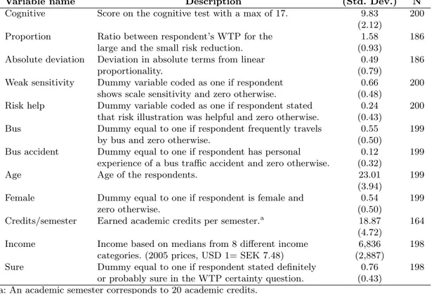
Descriptive statistics of our sample reveal that 54 percent of the participants were women and that the mean age was 23 years. The variable Cognitive is the cognitive test score, which has a mean of 9.83, and a lowest and highest score of 4 and 16, respectively. The sample mean of total amount of academic
credits earned is 51.10, and Credits/semester, which defines earned credits per semester, shows a slightly lower average than the required 20 credits for full time students, 18.87. Variables used in the analysis and descriptive statistics are found in Table 2. Since not all the respondents answered all the questions on individual characteristics and accident experience, some of the variables have fewer observations than 200.
[Table 2 about here.]
The variables Weak sensitivity, Proportion and Absolute deviation indicate how well, according to our hypothesis, respondents answered the survey. Weak sensitivity is a dummy variable which takes the value one if respondents state a higher WTP for the larger risk reduction than for the smaller one.
Proportion is a measure of the ratio between the WTP for the larger and smaller risk reductions, and Proportion is equal to 1.5 for fourteen percent of the sample and has a mean value of 1.58, which is
close to proportionality. Absolute deviation is estimated as the absolute difference between the WTP and risk-reduction ratios. For instance, since the ratio between the risk reductions is 1.5, a WTP ratio of 1.75 or 1.25 will mean an absolute deviation of 0.25.
Fourteen of the respondents stated a zero WTP for both risk reductions. The follow-up questions for the zero-answers indicated that 12 zero-answers were “true” (“risk reduction too small” or “cannot afford to pay”) and that 2 were protest answers (“question unclear” or “WTP should not be used”). Regarding the variables which indicate experience of the good, Bus and Bus accident, 55 percent of the respondents frequently took the bus, and 12 percent had personal experience of some sort of bus accident.
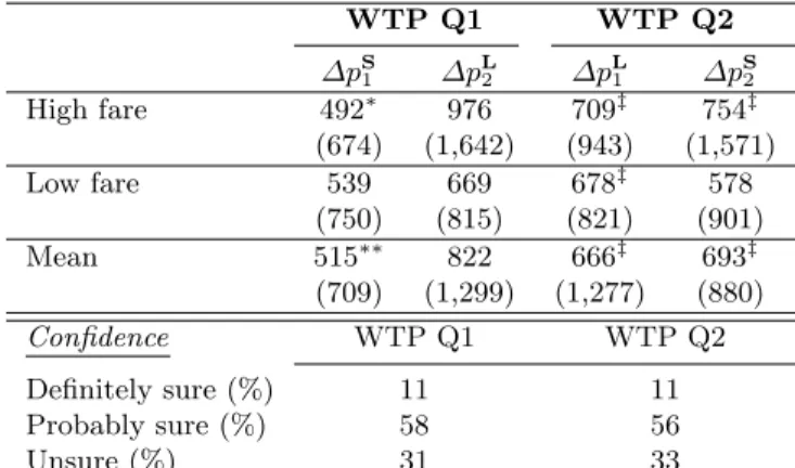
The answers to the WTP questions are shown in Table 3, where the mean estimates of the WTP answers to the first question show that the respondents had a higher WTP for the larger risk reduction than for the smaller one. Moreover, the results reveal no statistically significant framing effect from the different bus fares on mean WTP. However, the results indicate a starting point bias. Respondents who first stated their WTP for the larger risk reduction (Large Risk ), stated a higher WTP for the smaller risk reduction than those respondents who were first asked about their WTP for the smaller risk reduction, and vice versa.22The differences were not statistically significant, though.
[Table 3 about here.]
The relationships between Cognitive and Weak sensitivity, and Absolute deviation are examined in Table 4.23The highest scoring group has the highest share of respondents showing weak scale sensitivity and the lowest absolute deviation from linear proportion. For instance, in the specification with two groups, 77 and 59 percent show weak scale and the deviation is 0.38 and 0.57 for the high (11-16) and low (4-10) score groups, respectively, differences which are statistically significant. As can further be seen,
the share of respondents showing weak scale decreases and the deviation increases in size for groups with lower cognitive scores. A comparison of geometric means also showed that the results were not sensitive to outliers. Moreover, there is no clear pattern between Cognitive and Credits/semester. Partial correlation analysis between Cognitive and Credits/semester also shows no statistically significant correlation.
[Table 4 about here.]
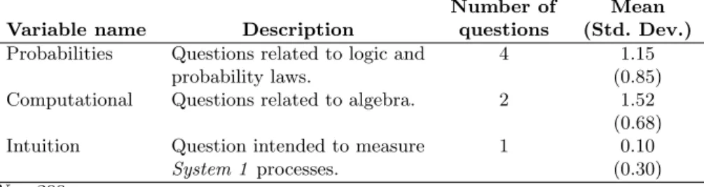
Based on the factor analysis three variables measuring different aspects of cognitive abilities were also used in the analysis of scale sensitivity. The factor analysis indicated a first factor which was dependent on four questions, where three of them measured primarily System 2 processes of understanding the logic of probabilities (Bayes’ theorem and law of large numbers) and the fourth question was a general quiz question on logic, and we label this variable Probabilities.24 The second variable created based on the factor analysis identification consists of two questions measuring pure computational ability, or algebra, and we label it Computational. A third factor was almost only dependent on one single questions, the example from Frederick (2005) mentioned in the last section, and since it was the most pure System 1 related question we call it Intuition and include it as a single dummy variable.
[Table 5 about here.]
4.2 Regression Analysis
We start this section by analyzing how the respondents’ first WTP answers are affected by different attributes using multivariate OLS. Multivariate probit and OLS regressions are then run to test for weak and strong scale sensitivity. Three different specifications regarding cognitive ability are used in these regressions: (i) Cognitive, (ii) the variables created from the factor analysis, Probability, Computational and Intuition, and (iii) to allow for non-linearity, Cognitive divided into four different categories based on test scores from Table 4, with the group with the lowest score as the reference group. Functional forms of the regressions were determined by goodness-of-fit and diagnostic tests.
The results of the WTP regressions are presented in Table 6. In the two regressions on the whole sample WTP for the larger risk reduction (Large risk ) is statistically significantly higher than for the smaller reduction. The coefficient estimates are 0.42 and 0.41, which implies a 52 and 51 percent higher WTP for the larger risk reduction. We cannot reject the hypothesis that WTP is proportional to the size of the risk reduction in either of the regressions. All the other coefficient estimates of the covariates are statistically insignificant. Among other things, the result implies that WTP is not related to cognitive ability, independent of measured by Cognitive or by the variables from the factor analysis, Probability,
To further examine the relationship between WTP and cognitive ability the sample was divided into four subgroups (the same groups as in Table 4) based on the respondents’ test score. We find a statistically significant higher WTP for the larger risk reduction only in the groups with test scores 9-10 and 12-16. The coefficient estimates are 0.50 and 0.69 which imply that the WTP for the larger risk reduction is 65 and 100 percent higher in the 9-10 and 12-16 group, respectively. We cannot reject, however, that WTP is proportional to the size of the risk reduction. Thus, both groups pass the weak and strong scale sensitivity tests. Moreover, in the highest scoring group we find that respondents who have bus-accident experience state a higher WTP, and those who found the visual aid helpful (Risk help) state a lower WTP.
[Table 6 about here.]
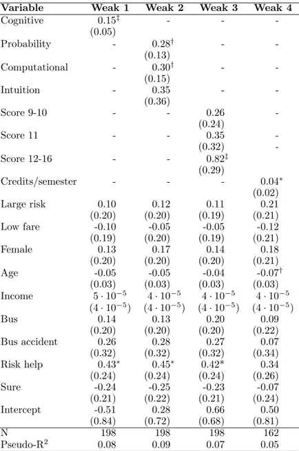
Whereas the analysis of WTP so far has been between-tests, we now move on to within-tests of scale sensitivity. The results of the probit regressions on Weak sensitivity are shown in Table 7. A positive coefficient indicates a higher probability of showing weak scale sensitivity, i.e. stating a higher WTP for the larger risk reduction. The results in the first column show that a higher score on the cognitive test is associated with a higher probability of showing weak scale sensitivity. The second specification, with cognitive ability divided into three variables, a higher score on the probability related variable as well as computational related variable is positively related to showing weak scale sensitivity. In third specification, when Cognitive was recorded into binary variables, we find that coefficient estimates are increasing with cognitive score, but only statistically significantly for the group with the highest test score. In other words, only the group with the best test score is statistically significantly more likely than the group with the lowest test score to show weak scale sensitivity. Moreover, in these specifications, respondents who stated that the risk illustration in the questionnaire was helpful when they answered the WTP questions (Risk help), are more likely to show weak scale sensitivity. In the last regression in Table 7 we see that the coefficient sign for Credits/semester is also positive and statistically significant. However, the impact is quite small.
[Table 7 about here.]
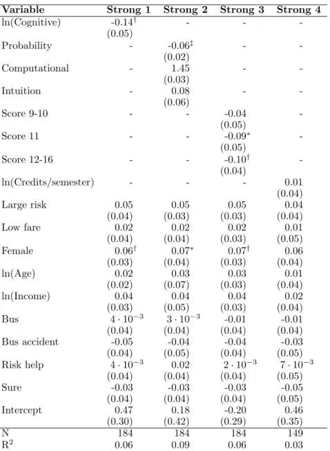
Regarding strong scale, the results in Table 4 indicate a positive relationship between strong scale sensitivity and cognitive ability. The test for strong scale sensitivity is further conducted by examining the correlation between Absolute deviation and different explanatory variables. As explained in section 2, WTP should be increasing and concave, i.e. Proportion ∈ (1, 1.5), and near-proportional to the size of the risk reduction, i.e. close to 1.5. Restricting the sample to respondents with Proportion ∈ (1, 1.5) only gives us 21 observations, however. Thus, very few respondents’ WTP was strictly increasing and concave.
We did not find any statistically significant relationships for this small group and we, therefore, decided to analyze the deviation from proportionality for the whole sample. In the analysis, negative coefficient estimates indicate a more near-proportional WTP.
The results are shown in Table 8, and the same pattern as in the test for weak scale sensitivity appears. A higher cognitive score implies less deviation from proportionality. In the second specification we see that a higher score on Probability is significantly associated with a more near-proportional WTP. No significant association can be found for Computational or Intuition. In the third specification we also see that groups with higher cognitive scores show lower deviation from proportionality, a deviation which is statistically significant for the two highest scoring groups. In the fourth specification, the coefficient sign for Credits/semester is not statistically significant. Moreover, the coefficient for Female is positive and statistically significant in three of the regressions, which means that male respondents stated a more near-proportional WTP.25
[Table 8 about here.]
5 Discussion
The results of this study support our hypothesis, that more cognitively skilled respondents will give answers less flawed by scale bias. When analyzing both the descriptive statistics and the regression results, respondents scoring higher in the cognitive ability test gave answers less flawed by scale bias. However, in the test for strong scale sensitivity only 21 out of 200 respondents (10 percent) stated a WTP that was increasing and strictly concave with with the size of the risk reduction, and we, therefore, treated positive as well as negative deviations from proportionality as equals. Our strong scale sensitivity test should, therefore, be seen as a test of deviation from proportionality, where we allow for positive “errors” in both directions, i.e. WTP ratios outside the 1 − 1.5 range.
Since the policy implications might be different, depending on the explanations for the results, it is important to discuss the underlying reasons for them. An alternative hypothesis to the one tested in this study, i.e. that scale sensitivity is related to cognitive ability, is that our findings are a result of more motivated respondents being more eager to do well in the cognitive test and thinking over the WTP questions more carefully. Thus, the respondents with low cognitive scores might not have had less cognitive ability, but might have been less motivated during the experiment. In an attempt to single out which parts of the cognitive test that was most important for the results, factor analysis was used. On the basis of this analysis, we found indications that respondents’ test score on the questions demanding skills in probability laws, rather than e.g. pure computational ability, was most importantly related to scale sensitivity. The result that it was certain parts of the cognitive test, rather than the full test,
which was significantly associated with scale sensitivity, indicates that motivation might not explain our results. This would mean that exogenous differences in cognitive ability among respondents might be a motivating factor for our results, and thus, respondents with lower cognitive ability might have a harder time grasping the scenario and the concept of WTP for risk reductions. Note that our results do not tell us how people with lower cognitive ability behave in real market situations, only that they might find it harder to grasp this kind of hypothetical scenarios.
Given that cognitive ability seems to be important for scale sensitivity, it seems difficult to overcome this problem by simply improving the survey designs and the policy implications are uncertain. One policy implication could be that it is necessary to test the respondents’ probability comprehension and to exclude those who fail the test from the analysis. A problem with such an approach is that there is a risk that the estimated values might not be representative of the targeted population. Another policy implication would be, that a minimum requirement in SP-studies on risk reductions should be to include an example scenario where the analyst carefully explains the nature of tradeoffs between probability changes and other consumption to the respondents. This is already today included in many studies, and together with the use of believable survey scenarios and risk illustrations, it will increase the understanding of the hypothetical scenario with the potential to mitigate the dependency on cognitive ability for scale sensitivity.
Questions on preference certainty are usually employed in closed-ended surveys, and the existing empirical evidence indicates that the hypothetical bias tends to be smaller among respondents who are more sure of their answer, which results in a lower stated WTP for this group (Blumenschein et al., 1998, 2001, 2005; Champ et al., 1997; Champ and Bishop, 2001). In our study where we use open-ended questions the variable used to analyze preference uncertainty was, however, insignificant in all the regressions, including the WTP regression. Moreover, the respondents who stated that the risk illustration (Risk help) was helpful were also more likely to show weak scale sensitivity. An analysis of Risk help did not provide us with any clear answers to why the risk illustration was considered helpful. Among other things, we did not find that the risk illustration was helpful for those with better understanding of probabilities.
Standard scale tests in the literature generally focus on the comparison of different sub-samples that have stated WTP for different risk reductions (between-tests). In this paper we primarily focus on scale tests on individual level, i.e. an internal scale test (within-test). A critique against within-tests is that they are irrelevant and meaningless since it is hard to imagine that an internal scale test will not pass a validity test of at least weak scale sensitivity (NOAA, 1993; Hammar and Johansson-Stenman, 2004). This was also supported by findings in Frederick and Fischhoff (1998), one of few studies that have
examined within- and between-tests, where they showed that within-tests lead to more scale sensitivity (Frederick and Fischhoff, 1998). However, 36.5 percent of the respondents showed no scale sensitivity at all in our study and only 10 percent stated a WTP that was increasing and concave with the size of the risk reduction, i.e. as predicted by economic theory. Our data clearly demonstrate that the assumption that within-tests necessarily pass a scale test is an all too optimistic assumption. This has also been shown in the literature review conducted in Hammitt and Graham (1999), where they also point out the fact that plenty of respondents state the same WTP, even if they get to answer different risk reduction questions after one another. Moreover, Bateman and Brouwer (2006) asked respondents to state their WTP to reduce skin-cancer risk for themselves and their household and tested for weak scale sensitivity. They used a split sample design, and “[i]n summary” (p. 210) found weak scale sensitivity in a subsample that received dichotomous choice questions, but in contrast to our findings, no weak scale sensitivity in a subsample that answered open-ended questions.
Between-tests are, however, important when VSL (or any other non-marketed amenity) is estimated for policy purposes. A weakness with the standard between-tests is that they focus on average values, which do not necessarily reveal anything about the consistency and internal validity of each respon-dent’s WTP. Large positive and negative deviations might result in a near-proportionality of the mean estimate.26 We could not reject proportionality in the WTP regression, and thus near-proportionality could not be rejected using between-tests in our study. Within-tests measure the validity of each indi-vidual’s stated WTP to a larger degree, and we, therefore, argue that within- and between-tests are not substitutes but rather complements, and that internal scale tests can be important as validity tests of respondents’ preferences. However, it is important in internal validity tests to be aware of the proba-bility that respondents had the opportunity to give answers they believed were “correct” but did not necessarily reflect their preferences.
Finally we briefly discuss the VSL elicited from this study. The population mean VSL estimate on the basis of only the WTP answers to the first WTP question, which is not affected by any starting point bias, is SEK 13.4 million. This can be compared with the official Swedish VSL for the transport sector which is SEK 17.1 million (SIKA, 2005), a value which originates from an early CVM-study by Persson and Cedervall (1991). From Persson et al. (2001) the preferred VSL was equal to SEK 24.4 million. Johannesson et al. (1996) and Hultkrantz et al. (2006) estimated VSL for a risk reduction as both a private and a public good. The private and the public good estimates in Johannesson et al. (1996) were SEK 48.7 and 36.2 million, whereas in Hultkrantz et al. (2006) they were 53.2 and 20.2, respectively.27 The result is more similar to that of a recent Swedish RP-study where marginal WTP for car safety was estimated (Andersson, 2005). VSL in that study was estimated at SEK 13.1 million.
A comparison of VSL estimates from different studies is always problematic, since the values are context related. Comparison with Swedish CVM-studies might not be very informative, since they are all flawed by scale bias. Moreover, in this study we ask about bus mortality risk, whereas Andersson (2005) examines car mortality risk. Bus mortality risk is not a pure private good, and there is a risk that values also represent paternalistic altruism (safety orientated) or that respondents answer strategically when they state their WTP for that kind of risk reduction, which also makes comparison with the value in Andersson (2005) difficult. Note that, since we conducted within-tests on scale sensitivity, our findings should not be affected by potential strategic bias, altruism, or whether stated WTP also reflects preferences to reduce injury risk (the respondent’s both answers should be affected to the same relative degree). How the student population can affect VSL studies in general is also somewhat uncertain. There is some evidence that a hypothetical bias is a more severe problem in student samples (Murphy et al., 2005). Even though the aim of this paper is not to elicit a VSL for policy purposes, our values seem reasonable given our sample and compared with other recent Swedish studies, which (together with results on scale sensitivity) can be regarded as a validity test of our experiment.
Acknowledgements The authors would like to thank Lars Hultkrantz, Gunnar Isacsson, Gunnar Lindberg, Fridtjof Thomas, seminar participants at VTI, Karlstad University, ¨Orebro University and Gothenburg Uni-versity, and conference participants at the “27thNordic Health Economists’ Study Group Meeting” for valuable
comments and support. Financial support from the Swedish National Road Administration is gratefully acknowl-edged. The authors are solely responsible for the results and views expressed in this paper.
Notes
1Scale and scope are used interchangeably in the literature to define the size of the good. We choose to
use scale, since it dominates in the literature on mortality risk reductions. This also complies better with the definitions on scale and scope in production theory.
2The effect of the baseline risk (p) on VSL is often referred to as the “dead-anyway effect” (Pratt and
Zeckhauser, 1996). For an analysis on how VSL is affected by aversion to financial risks, see Eeckhoudt and Hammitt (2004).
3 VSL(∆p)
VSL =
[ua(w)−ud(w)]/[(p−∆p)u0d(w)+(1−(p−∆p))u0a(w)] [ua(w)−ud(w)]/[pu0d(w)+(1−p)u0a(w)] =
1 1+∆p ±· u0a(w) u0a(w)−u0d(w) −p ¸
4The experiment included students from the following disciplines; business administration, economics, human
resources, teaching and political science. Most of these students were business majors (70 percent). A preliminary analysis showed that the area of study had no significant influence on either the cognitive test or the WTP answers, and the analysis based on area of study is, therefore, omitted.
5All prices in the paper are 2005 prices. USD 1 = SEK 7.48 (December 2005, www.riksbanken.se, 01/27/06.) 6This person was Mikael Svensson, one of the authors.
7More detailed information about the experiment, e.g. questions used in the test on cognitive ability, the
CVM-survey design, etc., is available upon request from the authors.
8Our test is a crude measure of cognitive ability, and content areas such as verbal reasoning, figural reasoning
or short-term memory, which are also thought to be important aspects of mental and cognitive ability, are not tested. The questions used can be found in previous experiments and are similar to those used in intelligence tests (Frederick, 2005; Kahneman and Tversky, 1972, 1983; Rabin, 2002).
9Frederick (2005) used three questions in his test.
10In the words of Frederick (2005, p. 26): “System 1 processes occur spontaneously and do not require or
consume much attention. Recognizing that the face of the person entering the classroom belongs to your math teacher involves System 1 processes.”.
11This question was taken from the three-item cognitive test reported in Frederick (2005).
12This can be performed either by using the “regression method” or the Bartlett scoring method (Barthomolew,
1987).
13It has been found that student self-discipline better predicts grades than student IQ (Duckworth and
Selig-man, 2005; Wolfe and Johnson, 1995).
14A full semester corresponds to 20 credits. Since a Swedish academic year consists of two semesters, a full-time
student is supposed to acquire 40 credits per year.
15Our analysis also showed that the total numbers of academic credits had no significant effect in the regressions. 16The campus at Karlstad University is located approximately 9 kilometers (ca. 5.6 miles) from the city center
and the students often use the bus in order to get to/from the university and/or city center.
17We decided to use a baseline risk of an age group other than the respondents’ own. The risk of a 50 year-old
was used by both Persson et al. (2001) and Carlsson et al. (2004), which is why we decided to use the risk of that particular age group.
18The annual bus fare at the time of the survey in Karlstad was SEK 3,690. 19The question has been freely translated from Swedish to English by the authors.
20The survey asks about the city council selecting from one of three bus companies that are distinguished by
the levels of safety, when contracting out the service to a private firm. This corresponds to the actual procedure in the city of Karlstad as well as most other Swedish cities.
21Protests answers can have different explanations. For instance, that the respondent has problems
understand-ing the hypothetical scenario, or that the respondent objects to the fact that a monetary value can be placed on the non-marketed amenity.
22This is contrary to what has been found for environmental public goods, where the WTP for the smaller
quantity was larger if presented first (for references, see Clark and Friesen, 2006).
23The intention was to divide the sample into equal-sized groups based on the test result. However, the test
score is made up of integers, which is why the group sizes differ.
24The qualitative results of scale sensitivity in section 4.2 also hold if Probabilities only includes the first two
and/or three of the questions instead of all four.
25Excluding the covariates Bus, Bus accident, Risk help and Sure from the regressions in Tables 7 and 8 resulted
in a statistically significant coefficient estimate for Female also in the fourth specification in Table 8. Apart from that result, the effect on the coefficient estimates was negligible.
26A result we also got in this study when group comparisons, based on the groups in Table 4, of Proportionality
were conducted.
27Johannesson et al. (1996) show a range of SEK 30-59 million for the private good and SEK 17-49 million for
References
Alberini, A., M. Cropper, A. Krupnick, and N. B. Simon: 2004, ‘Does the Value of a Statistical Life Vary With the Age and Health Status?: Evidence from the USA and Canada’. Journal of Environmental
Economics and Management 48(1), 769–792.
Andersson, H.: 2005, ‘The Value of Safety as Revealed in the Swedish Car Market: An Application of the Hedonic Pricing Approach’. Journal of Risk and Uncertainty 30(3), 211–239.
Barthomolew, D. J.: 1987, Latent Variable Models and Factor Analysis. New York, NY, USA: Oxford University Press.
Bateman, I. J. and R. Brouwer: 2006, ‘Consistency and construction in stated WTP for health risk reductions: A novel scope-sensitivity test’. Resource and Energy Economics 28(3), 199–214.
Benjamin, D. J. and J. M. Shapiro: 2005, ‘Does Cognitive Ability Reduce Psychological Bias?’. Harvard University, Mimeo.
Blumenschein, K., G. C. Blomquist, M. Johannesson, N. Horn, and P. Freeman: 2005, ‘Eliciting Will-ingness to Pay without Bias: Evidence from a Field Experiment’. Mimeo, University of Kentucky, Lexington, KY, USA.
Blumenschein, K., M. Johannesson, G. C. Blomquist, B. Liljas, and R. M. O’Conor: 1998, ‘Experimental Results on Expressed Certainty and Hypothetical Bias in Contingent Valuation’. Southern Economic
Journal 65(1), 169–177.
Blumenschein, K., M. Johannesson, K. K. Yokoyama, and P. R. Freeman: 2001, ‘Hypothetical versus real willingness to pay in the health care sector: results from a field experiment’. Journal of Health
Economics 20(3), 441–457.
Carlsson, F., O. Johansson-Stenman, and P. Martinsson: 2004, ‘Is Transport Safety More Valuable in the Air’. Journal of Risk and Uncertainty 28(2), 147–163.
Carson, R. T., N. E. Flores, and N. F. Meade: 2001, ‘Contingent Valuation: Controversies and Evidence’.
Environmental and Resource Economcis 19(2), 173–210.
Carson, R. T. and R. C. Mitchell: 1995, ‘Sequencing and Nesting in Contingent Valuation Surveys’.
Journal of Environmental Economics and Management 28(2), 155–173.
Champ, Patricia A. and, B. R. C., T. C. Brown, and D. W. McCollum: 1997, ‘Using Donation Mechanisms to Value Nonuse Benefits from Public Goods’. Journal of Environmental Economics and Management 33(2), 51–162.
Champ, P. A. and R. C. Bishop: 2001, ‘Donation Payment Mechanism and Contingent Valuation: An Empirical Study of Hypothetical Bias’. Environmental and Resource Economics 19(4), 383–402.
Clark, J. and L. Friesen: 2006, ‘The Causes of Order Effects in Contingent Valuation Surveys: An Experimental Investigation’. University of Canterbury, New Zealand, Mimeo.
Corso, P. S., J. K. Hammitt, and J. D. Graham: 2001, ‘Valuing Mortality-Risk Reduction: Using Visual Aids to Improve the Validity of Contingent Valuation’. Journal of Risk and Uncertainty 23(2), 165– 184.
Desvousges, W. H., J. F. Reed, R. W. Dunford, K. J. Boyle, S. P. Hudson, and K. N. Wilson: 1993,
Contingent Valuation: A Critical Assessment, Chapt. Measuring Natural Resource Damage with
Con-tingent Valuation: A Test of Validity and Reliability, pp. 91–159. Amsterdam, The Netherlands: Norht-Holland.
Diamond, P. A. and J. A. Hausman: 1994, ‘Contingent Valuation: Is Some Number Better than No Number?’. Journal of Economic Perspective 8(4), 45–64.
Duckworth, A. L. and M. E. Seligman: 2005, ‘Self-Discioline Outdoes IQ in Predicting Academic Perfor-mance of Adolescents’. Psychological Science 16(12), 939–944.
Eeckhoudt, L. R. and J. K. Hammitt: 2004, ‘Does Risk Aversion Increase the Value of Mortality Risk?’.
Journal of Environmental Economics and Management 47(1), 13–29.
Epstein, S.: 1994, ‘ntegration of the Cognitive and Psychodynamic Unconscious’. American Psychologist 49(8), 709–724.
Frederick, S. and B. Fischhoff: 1998, ‘Scope (In)sensitivity in Elicited Valuations’. Journal of Risk,
Decision and Policy 3(2), 109–123.
Frederick, S.: 2005, ‘Cognitive Reflection and Decision Making’. Journal of Economic Perspectives 19(4), 25–42.
Green, D., K. E. Jacowitz, D. Kahneman, and D. McFadden: 1998, ‘Referendum contingent valuation anchoring and willingness to pay for public goods’. Resource and Energy Economics 20(2), 85–116. Hammar, H. and O. Johansson-Stenman: 2004, ‘The value of risk-free cigarettes - do smokers
underes-timate the risk?’. Health Economics 13(1), 59–71.
Hammitt, J. K. and J. D. Graham: 1999, ‘Willingness to Pay for Health Protection: Inadequate Sensitivity to Probability?’. Journal of Risk and Uncertainty 18(1), 33–62.
Hammitt, J. K.: 2000a, ‘Evaluating Contingent Valuation of Environmental Health Risks: The Propor-tionality Test’. AERE (Association of Environmental and Resource Economics) Newsletter 20(1), 14–19.
Hammitt, J. K.: 2000b, ‘Valuing Mortality Risk: Theory and Practice’. Environmental Science &
Hanemann, W. M.: 1994, ‘Valuing the Environment Trough Contingent Valuation’. Journal of Economic
Perspectives 8(4), 19–43.
Heberlein, T. A., M. A. Wilson, R. C. Bishop, and N. C. Schaeffer: 2005, ‘Rethinking the Scope Test as a Criterion for Validity in Contingent Valuation’. Journal of Environmental Economics and Management 50(1), 1–22.
Hultkrantz, L., G. Lindberg, and C. Andersson: 2006, ‘The Value of Improved Road Safety’. Journal of
Risk and Uncertainty 32(2), 151–170.
Johannesson, M., P.-O. Johansson, and R. M. O’Connor: 1996, ‘The Value of Private Safety Versus the Value of Public Safety’. Journal of Risk and Uncertainty 13(3), 263–275.
Jones-Lee, M. W.: 1974, ‘The Value of Changes in the Probability of Death or Injury’. Journal of Political
Economy 82(4), 835–849.
Kahneman, D. and S. Frederick: 2002, Heuristics and Biases: The Psychology of Intuitive Judgment, Chapt. Representativeness Revisited: Attribute Substitution in Intuitive Judgment., pp. 49–81. Cam-bridge University Press.
Kahneman, D. and J. L. Knetsch: 1992, ‘Valuing Public goods: The Purchase of Moral Satisfaction’.
Journal of Environmental Economics and Management 22(1), 57–70.
Kahneman, D., I. Ritov, and D. Schkade: 1999, ‘Economic Preferences or Attitude Expressions?: An Analysis of Dollar Responses to Public Issues’. Journal of Risk and Uncertainty 19(1-3), 203–235. Kahneman, D., P. Slovic, and A. Tversky: 1982, Judgement under Uncertainty: Heuristics and Biases.
New York, NY, USA: Cambridge University Press.
Kahneman, D. and A. Tversky: 1972, ‘Subjective Probability: A Judgement of Representativeness’.
Cognitive Psychology 3(3), 430–454.
Kahneman, D. and A. Tversky: 1983, ‘Can irrationality be intelligently discussed?’. Behavioral and Brain
Sciences 6, 509–510.
Kahneman, D.: 2003, ‘Maps of Bounded Rationality: Psychology for Behavioral Economics’. American
Economics Review 93(5), 1449–1475.
Lawley, D. N. and A. E. Maxwell: 1963, Factor Analysis as a Statistical Method. London,UK: Butter-worths.
Murphy, J. J., P. G. Allen, T. H. Stevens, and D. Weatherhead: 2005, ‘A Meta-Analysis of Hypothetical Bias in Stated Preference Valuation’. Environmental and Resource Economics 30(3), 313–325. NOAA: 1993, ‘Report of the NOAA Panel on Contingent Valuation’. Federal Register 58, Arrow, K,
Persson, U. and M. Cedervall: 1991, ‘The Value of Risk Reduction: Results of a Swedish Sample Survey’. IHE Working Paper 1991:6, The Swedish Institute for Health Economics.
Persson, U., A. Norinder, K. Hjalte, and K. Gral´en: 2001, ‘The Value of a Statistical Life in Transport: Findings from a new Contingent Valuation Study in Sweden’. Journal of Risk and Uncertainty 23(2), 121–134.
Pratt, J. W. and R. J. Zeckhauser: 1996, ‘Willingness to Pay and the Distribution of Risk and Wealth’.
Journal of Political Economy 104(4), 747–763.
Rabin, M.: 2002, ‘Inference by Believers in the Law of Small Numbers’. Quarterly Journal of Economics 117(3), 775–816.
Rosen, S.: 1988, ‘The Value of Changes in Life Expectancy’. Journal of Risk and Uncertainty 1(3), 285–304.
SIKA: 2005, ‘Kalkylv¨arden och kalkylmetoder - En sammanfattning av Verksgruppens rekommendationer 2005’. Pm 2005:16, SIKA (Swedish Institute for Transport and Communications Analysis), Stockholm, Sweden.
Sloman, S.: 1996, ‘The Empirical Case for Two Systems of Reasoning’. Psychological Bulletin 119(1), 3–22.
Smith, V. K.: 1992, ‘Arbitrary Values, Good Causes, and Premature Verdicts’. Journal of Environmental
Economics and Management 22(1), 71–89.
Stanovich, K. and R. West: 2000, ‘Individual differences in reasoning: Implications for the rationality debate?’. Behavioral and Brain Sciences 23, 645–726.
Stanovich, K. and R. West: 2002, Heuristics and biases: The psychology of intuitive judgement, Chapt. Individual differences in reasoning: Implications for the rationality debate?, pp. 421–440. New York, NY, USA: Cambridge University Press.
Varian, H. R.: 1999, ‘Commentary on “Economic Preferences of Attitude Expressions?: An Analysis of Dollar Responses to Public Issues” by Kahneman et al.’. Journal of Risk and Uncertainty 19(1-3), 241–242.
Weinstein, M. C., D. S. Shepard, and J. S. Pliskin: 1980, ‘The Economic Value of Changing Mortality Probabilities: A Decision-Theoretic Approach’. Quarterly Journal of Economics 94(2), 373–396. Wolfe, R. and S. Johnson: 1995, ‘Personality as a Predictor of College Performance’. Education and
Fig. 1 The value of a statistical life: the marginal rate of substitution between mortality risk (p) and wealth (w), and WTP for a non-marginal risk reduction (∆p).
-6 1 p w VSL ÃÃÃÃÃÃ ÃÃÃÃÃÃ ÃÃÃÃÃ ³³∆p ³³ WTP 6
Fig. 2 Willingness to pay question with small risk reduction and low annual bus fare
We would first like to know how much you are willing to pay to travel with Bus
company B instead of Bus company A. The risks of accidents with fatal outcome for Bus companies A and B are:
– Bus company A: Risk = 10 per 100,000 – Bus company B: Risk = 6 per 100,000
An annual pass with Bus company A costs SEK 3,000 (SEK 250 × 12).
What is the maximum extra mount you are willing to pay per year to travel with Bus company B instead of Bus company A?
The maximum extra amount I am willing to pay is . . . SEK.
Are you definitely sure, probably sure or unsure regarding your answer (mark with an x)?
Table 1 Near-proportionality of WTP High baseline risk Low baseline risk
ph 0.01 pl 0.0001 ∆ph1 0.002 ∆pl1 0.00002 ∆ph2 0.005 ∆pl2 0.00005 ∆ph2 ∆ph1 2.5 ∆pl2 ∆pl1 2.5 WTPh1 2,231 WTPl1 22.44 WTPh2 5,472 WTPl2 56.06 WTPh2 WTPh1 2.453 WTPl2 WTPl1 2.498 WTP derived from EU0= EU1. ud(w) = ln(w) and ua(w) = 10 + 5ln(w) w = 100, 000
Table 2 Description of dependent and explanatory variables
Mean
Variable name Description (Std. Dev.) N Cognitive Score on the cognitive test with a max of 17. 9.83 200
(2.12)
Proportion Ratio between respondent’s WTP for the 1.58 186 large and the small risk reduction. (0.93)
Absolute deviation Deviation in absolute terms from linear 0.49 186
proportionality. (0.79)
Weak sensitivity Dummy variable coded as one if respondent 0.66 200 shows scale sensitivity and zero otherwise. (0.48)
Risk help Dummy variable coded as one if respondent stated 0.24 200 that risk illustration was helpful and zero otherwise. (0.43)
Bus Dummy equal to one if respondent frequently travels 0.55 199 by bus and zero otherwise. (0.50)
Bus accident Dummy equal to one if respondent has personal 0.12 199 experience of a bus traffic accident and zero otherwise. (0.32)
Age Age of the respondents. 23.01 199 (3.94)
Female Dummy equal to one if respondent is female and 0.54 199
zero otherwise. (0.50)
Credits/semester Earned academic credits per semester.a 18.87 164
(4.72)
Income Income based on medians from 8 different income 6,836 198 categories. (2005 prices, USD 1= SEK 7.48) (2,887)
Sure Dummy equal to one if respondent stated definitely 0.76 198 or probably sure in the WTP certainty question. (0.43)
Table 3 Willingness to pay and preference uncertainty WTP Q1 WTP Q2 ∆pS 1 ∆pL2 ∆pL1 ∆pS2 High fare 492∗ 976 709‡ 754‡ (674) (1,642) (943) (1,571) Low fare 539 669 678‡ 578 (750) (815) (821) (901) Mean 515∗∗ 822 666‡ 693‡ (709) (1,299) (1,277) (880) Confidence WTP Q1 WTP Q2 Definitely sure (%) 11 11 Probably sure (%) 58 56 Unsure (%) 31 33
WTP Q1 and WTP Q2 refer to the first and second WTP questions. Respondents who in Q1 stated their WTP for ∆pS
1, in Q2 stated their WTP for ∆pL1, and vice versa. Superscripts S and L refer to small and large risk
reductions, and subscripts 1 and 2 refer to sample group.
VSL in million SEK, and WTP and VSL in 2005 price level. USD 1= SEK 7.48 Standard deviations in parenthesis.
H0 : ∆pS= ∆pL; ** significant at 0.05 level, * significant at 0.10 level
H0 : WTPiQ1 = WTPiQ2; ‡ significant at 0.01 level, i ∈ {1, 2}
Framing effect of different bus fares not statistically significant.
WTP Q1 and WTP Q2 for same ∆p, and given the same bus fare, not statistically significantly different. Wilcoxon rank-sum employed for mean comparisons.
Table 4 Cognitive score, weak sensitivity, deviation from proportionality and credits per semester Cognitive Weak sensitivity Absolute deviation Credits/semester
score Mean N Mean N Mean N 12-16 0.81b 43 0.37e 42 19.55 34 11 0.70 30 0.40 30 18.26 22 9-10 0.62 77 0.55 68 18.47 65 4-8 0.54 50 0.58 46 19.24 43 9-11a 0.64c 107 0.51f 98 18.42 87 11-16 0.77d 73 0.38g 72 19.04 56 4-10 0.59 127 0.57 114 18.78 108 Full sample 0.66 200 0.49 186 18.87 164 Values for Weak sensitivity; share of respondents showing weak scale sensitivity. a: Cognitive score groups (CSG) 9-10 and 11 grouped together.
b: Statistically significantly different from CSG 4-8 and 12-16 at 0.01 and 0.05 level, respectively. c: Statistically significantly different from CSG 4-8 and 12-16 at 0.05 and 0.01 level, respectively. d: Statistically significantly different from CSG 4-10 at 0.05 level.
e: Statistically significantly different from CSG 4-8 at 0.05 level.
f: Statistically significantly different from CSG 4-8 and 12-16 at 0.1 and 0.05 level, respectively. g: Statistically significantly different from CSG 4-10 at 0.1 level.
Cognitive score and Credits/Semester not statistically significantly correlated. Wilcoxon rank-sum employed for mean comparisons.
Table 5 Descriptive Statistics for Variables based on Factor Analysis results Number of Mean Variable name Description questions (Std. Dev.) Probabilities Questions related to logic and 4 1.15
probability laws. (0.85) Computational Questions related to algebra. 2 1.52
(0.68) Intuition Question intended to measure 1 0.10
System 1 processes. (0.30)
N = 200
Table 6 Regression results WTP to reduce bus-mortality risk All Cognitive score
Variable respondents 4-8 9-10 11 12-16 ln(Cognitive) 0.22 - - - - -(0.34) Probability - 0.07 - - - -(0.10) Computational - 0.09 - - - -(0.12) Intuition - -0.18 - - - -(0.27) Large risk 0.42‡ 0.41† -0.01 0.50∗ 0.33 0.69† (0.16) (0.16) (0.42) (0.29) (0.48) (0.29) Low fare -0.21 -0.20 -0.13 -0.34 -0.19 0.08 (0.16) (0.16) (0.43) (0.29) (0.42) (0.31) Female -0.08 -0.07 0.12 0.01 0.38 -0.27 (0.16) (0.17) (0.41) (0.29) (0.62) (0.31) ln(Age) 0.07 0.06 -1.01 0.11 -1.01 -0.35 (0.31) (0.31) (1.67) (0.38) (1.58) (1.31) ln(Income) -0.17 -0.17 -0.45 0.20 0.01 -0.03 (0.21) (0.21) (0.50) (0.37) (0.65) (0.46) Bus 0.02 0.01 0.15 -0.19 0.68 -0.12 (0.17) (0.17) (0.45) (0.31) (0.53) (0.33) Bus accident 0.07 0.04 -0.53 -0.26 0.15 1.15† (0.25) (0.25) (0.65) (0.53) (0.53) (0.45) Risk help -0.24 -0.26 0.08 -0.18 -0.20 -0.80† (0.19) (0.20) (0.49) (0.34) (0.57) (0.38) Sure 0.28 0.28 0.24 0.32 0.77 -0.08 (0.18) (0.18) (0.43) (0.32) (0.53) (0.31) Intercept 6.56‡ 6.84‡ 12.84† 3.69 7.76 7.38∗ (2.05) (1.95) (6.00) (3.25) (6.37) (3.81) N 185 185 45 68 30 42 R2 0.08 0.09 0.10 0.11 0.06 0.19
Dependent variable, the natural logarithm of the WTP answer to the first WTP question. Two-tailed test: ‡ significant at 0.01 level, † at 0.05 level, * at 0.1 level.
Standard errors in brackets.
Large risk and Low fare are dummies equal to one if respondent in the first WTP
question stated his/her WTP for the larger risk reduction and was presented with the lower bus fare, respectively.
Table 7 Probit regression results: Weak scale sensitivity
Variable Weak 1 Weak 2 Weak 3 Weak 4
Cognitive 0.15‡ - - -(0.05) Probability - 0.28† - -(0.13) Computational - 0.30† - -(0.15) Intuition - 0.35 - -(0.36) Score 9-10 - - 0.26 -(0.24) Score 11 - - 0.35 -(0.32) -Score 12-16 - - 0.82‡ (0.29) Credits/semester - - - 0.04∗ (0.02) Large risk 0.10 0.12 0.11 0.21 (0.20) (0.20) (0.19) (0.21) Low fare -0.10 -0.05 -0.05 -0.12 (0.19) (0.20) (0.19) (0.21) Female 0.13 0.17 0.14 0.18 (0.20) (0.20) (0.20) (0.21) Age -0.05 -0.05 -0.04 -0.07† (0.03) (0.03) (0.03) (0.03) Income 5 · 10−5 4 · 10−5 4 · 10−5 4 · 10−5 (4 · 10−5) (4 · 10−5) (4 · 10−5) (4 · 10−5) Bus 0.14 0.13 0.20 0.09 (0.20) (0.20) (0.20) (0.22) Bus accident 0.26 0.28 0.27 0.07 (0.32) (0.32) (0.32) (0.34) Risk help 0.43∗ 0.45∗ 0.42* 0.34 (0.24) (0.24) (0.24) (0.26) Sure -0.24 -0.25 -0.23 -0.07 (0.21) (0.22) (0.21) (0.24) Intercept -0.51 0.28 0.66 0.50 (0.84) (0.72) (0.68) (0.81) N 198 198 198 162 Pseudo-R2 0.08 0.09 0.07 0.05
Dependent variable, Weak sensitivity.
Two-tailed test: ‡ significant at 0.01 level, † at 0.05 level, * at 0.1 level. Standard errors in brackets.
Large risk and Low fare are dummies equal to one if respondent in the first WTP
question stated his/her WTP for the larger risk reduction and was presented with the lower bus fare, respectively.
Table 8 Regression results: Strong scale sensititvy
Variable Strong 1 Strong 2 Strong 3 Strong 4
ln(Cognitive) -0.14† - - -(0.05) Probability - -0.06‡ - -(0.02) Computational - 1.45 - -(0.03) Intuition - 0.08 - -(0.06) Score 9-10 - - -0.04 -(0.05) Score 11 - - -0.09∗ -(0.05) Score 12-16 - - -0.10† -(0.04) ln(Credits/semester) - - - 0.01 (0.04) Large risk 0.05 0.05 0.05 0.04 (0.04) (0.03) (0.03) (0.04) Low fare 0.02 0.02 0.02 0.01 (0.04) (0.04) (0.03) (0.05) Female 0.06† 0.07∗ 0.07† 0.06 (0.03) (0.04) (0.03) (0.04) ln(Age) 0.02 0.03 0.03 0.01 (0.02) (0.07) (0.03) (0.04) ln(Income) 0.04 0.04 0.04 0.02 (0.03) (0.05) (0.03) (0.04) Bus 4 · 10−3 3 · 10−3 -0.01 -0.01 (0.04) (0.04) (0.04) (0.04) Bus accident -0.05 -0.04 -0.04 -0.03 (0.04) (0.05) (0.04) (0.05) Risk help 4 · 10−3 0.02 2 · 10−3 7 · 10−3 (0.04) (0.04) (0.04) (0.05) Sure -0.03 -0.03 -0.03 -0.05 (0.04) (0.04) (0.04) (0.05) Intercept 0.47 0.18 -0.20 0.46 (0.30) (0.42) (0.29) (0.35) N 184 184 184 149 R2 0.06 0.09 0.06 0.03
Dependent variable, the natural logarithm of the sum of perfect proportion (1.5) and Absolute deviation. The constant (1.5) was needed since we take logarithms. Two-tailed test: ‡ significant at 0.01 level, † significant at 0.05 level, * at 0.1 level. Robust standard errors in parenthesis.
Large risk and Low fare are dummies equal to one if respondent in the first WTP
question stated his/her WTP for the larger risk reduction and was presented with the lower bus fare, respectively.