The Valuation of Unlisted Equity
Master’s Thesis within: Business Administration Authors: Chakraborty Bidita
Hansson Victoria
Tutor: Manduchi Agostino
Wixe Sofia
i
Acknowledgements
Firstly, we would like to thank our tutors Agostino Manduchi and Sofia Wixe for their support and guidance through this process. We appreciate their encouragement and their help through problems encountered during our research.
We would also like to thank our fellow seminar students for their feedback and their help that has made it possible to improve this thesis.
………. ……….
Bidita Chakraborty Victoria Hansson
ii
Master Thesis in International Financial Analysis
Title: The Valuation of Unlisted EquityYear of publication: 2013
Author: Bidita Chakraborty & Victoria Hansson Tutor: Agostino Manduchi & Sofia Wixe
Subject terms: Valuation, Unlisted Equity, Price-to-Equity, Price-to-Book Value
Abstract
Background: A stakeholder of a company uses information related to the value of the company in order to make wiser business decisions. Defining a value for a business is of in-terest in several situations and for several stakeholders. A listed company, i.e. a company in which has its shares admitted to trading on a regulated market, is often valued based on market prices. For unlisted equity however the valuation is in general a more difficult task, as market prices are not readily available. The International Monetary Fund (IMF) puts forward the Balance of Payments and International Investment Position Manual, 6th ed. (BPM6) where seven equity valuation models are suggested. It is furthermore suggested that these models can be transferred and utilized on unlisted equity. This thesis aims to test the BPM6 methods on unlisted equity in Sweden between 2006 and 2012.
Purpose: The purpose of this thesis is to investigate the reliability of the suggested BPM6 valuation models, intended for listed companies, on unlisted companies in Sweden. A con-clusion regarding which model reflects the value of equity the best aims to be drawn. That model will subsequently be used in order to calculate a hypothetical market value. That val-ue will be compared to an actual one in the sense that the unlisted equity chosen for this study have all undergone an initial public offering (IPO), making a comparison possible. Method: This is solely a quantitative study. Firstly, a database consisting of peer groups, based on industry classifications, was created. The variables gathered in the various peer groups were all based on listed equity. The data underwent statistical tests in order to find the best regression model to predict market value for each industry and year. Five different regression models were tested, as alternatives to the Equity model and the Price-to-Book Value model. Secondly, the predicted value was compared to the actual value for the unlisted equity in order to test the reliability of the valuation models.
Conclusion: The result of this study shows that the model producing the most accurate prediction on equity value of unlisted companies is the multi-factor model. The model was based on a combination of earning and book value measures. Furthermore, this study shows that the predicted market values do not differ extensively from the actual market values, implying reliability. The results however produced some dispersion with both overestima-tions and underestimaoverestima-tions. Regardless of such results, the authors are able to draw a clear conclusion regarding the reliability. The authors conclude that the suggested models in the BPM6, put forward by IMF, serve as good indicators for valuing unlisted equity.
iii
Magisteruppsats inom Internationell Finansiell Analys
Titel: Värderingen av onoterade bolagPubliceringsår: 2013
Författare: Bidita Chakraborty & Victoria Hansson Handledare: Agostino Manduchi & Sofia Wixe
Nyckelord: Värdering, Onoterade bolag, Pris/vinst, Pris/bokfört värde
Abstrakt
Bakgrund: En intressent i ett företag använder information relaterat till värdet av bolaget för att göra förnuftiga affärsbeslut. Att definiera ett värde för en verksamhet är av intresse i flera situationer samt för olika intressenter. Ett noterat bolag, dvs. ett bolag som har sina ak-tier upptagna till handel på en reglerad marknad, värderas ofta baserat på marknadspriser. För onoterade aktier däremot är en värdering i allmänhet en svårare uppgift eftersom mark-nadspriser ofta är svårtillgängliga. Internationella Valutafonden (IMF) presenterar och före-slår användandet av sju värderingsmodeller i Balance of Payments and International
In-vestment Position Manual sjätte upplagan (BPM6). Vidare föreslås det att dessa modeller
kan överföras och användas på onoterade bolag. Denna avhandling syftar till att testa mo-dellerna på onoterade bolag i Sverige mellan 2006 och 2012.
Syfte: Syftet med denna avhandling är att undersöka tillförlitligheten i de föreslagna BPM6 värderingsmodellerna, avsedda för noterade bolag, på onoterade bolag i Sverige. En slutsats om vilken modell som speglar värdet av det egna kapitalet bäst önskas göras. Denna modell kommer senare att användas för att beräkna ett hypotetiskt marknadsvärde. Detta värde kommer att jämföras med ett faktiskt värde i den mening att de onoterade bolag som valts för denna studie har alla genomgått en börsintroduktion, vilket gör en jämförelse möjlig. Metod: Denna studie baseras endast på kvantitativ data. Först skapades en databas bestå-ende av branschindelade peer groups. De variabler som samlades i de olika grupperna var alla baserade på noterade bolag. Variablerna genomgick statistiska tester för att hitta den bästa regressionsmodellen till att förutsäga ett marknadsvärde för varje bransch och år. Fem olika regressionsmodeller testades, som alternativ till Pris/vinstmodellen och Pris/bokfört värdemodellen. Slutligen jämfördes de hypotetiska värdena med de faktiska värdena på de onoterade bolagen för att testa tillförlitligheten av BPM6 värderingsmodellerna.
Slutsats: Resultatet av denna studie visar att modellen som producerar det bästa förutsagda värdet på det egna kapitalet av de onoterade bolagen var multifaktormodellen. Modellen byggde på en kombination av inkomst och bokfört värde mått. Vidare visar denna studie att de hypotetiska marknadsvärdena inte skiljer sig mycket från de verkliga värdena, vilket in-nebär tillförlitlighet. Resultaten producerade dock viss spridning med både övervärderingar och undervärderingar. Oavsett spridningen, kan en tydlig slutsats göras gällande tillförlit-ligheten. Författarna drar slutsatsen att de föreslagna modellerna i BPM6, framtagna av IMF, verkar som goda modeller för att värdera onoterade bolag.
iv
Table of Contents
Acknowledgements ... i
Abstract ... ii
Abstrakt ... iii
1 Introduction ... 1
1.1 Background ... 1 1.2 Problem Discussion ... 2 1.3 Purpose ... 3 1.4 Delimitations ... 42
Theoretical Framework ... 5
2.1 Currently used Valuation Methods ... 5
2.2 BPM6 Equity Valuation Models ... 5
2.3 Models Included in this Study ... 6
2.3.1 Price to Earnings ... 6
2.3.2 Price to Book Value ... 6
2.3.3 Own Funds at Book Value (OFBV) ... 7
2.4 Models Excluded from this Study ... 8
2.4.1 Recent Transaction Price ... 8
2.4.2 Net Asset Value ... 8
2.4.3 Present Value of Earnings ... 9
2.4.4 Apportioning Global Value ... 9
2.5 Argumentation for delimitation of Models ... 9
2.6 Previous Research ... 10
2.7 Issues with Valuing Equity ... 10
2.8 Transferability ... 12
3
Method ... 14
3.1 Research Approach ... 14 3.2 Research Technique ... 14 3.3 Credibility ... 15 3.3.1 Reliability ... 15 3.3.2 Validity ... 15 3.4 Data Collection ... 15 3.5 Model Analysis ... 19 3.6 Hypotheses Testing ... 213.7 Analyzing the data ... 21
4
Empirical Results ... 23
4.1 Characteristics of Data Sample ... 23
4.2 Summary of the Statistical Procedure ... 23
4.3 Results of Regression Models ... 25
4.3.1 Results for 2006 ... 25
4.3.2 Results for 2007 ... 25
4.3.3 Results for 2008 ... 27
4.3.4 Results for 2010 & 2011 ... 28
4.4 Summary of Hypotheses ... 29
v
5
Analysis ... 32
6
Discussion ... 37
7
Conclusion ... 39
References ... 40
Appendices ... 42
vi
Figures, Tables and Appendices
Figure 4-1. Distribution of industries for the study ... 23
Figure 4-2. Scatterplot of Market Values ... 31
Figure 5-1. Graphical interpretations of the disparity of results ... 34
Table 1. GICS Industry Classifications ... 17
Table 2. Variables included in Regression analysis ... 18
Table 3. Regression Models on Market Value of Equity ... 20
Table 4. Coefficients for ‘Financials’ Mid Cap 2006 ... 25
Table 5. Coefficients for ‘Industrials’ Mid Cap 2006 ... 25
Table 6. Coefficients for ‘Industrials’ Mid Cap 2007 ... 26
Table 7. Coefficients for ‘Industrials’ Small Cap 2007 ... 27
Table 8. Coefficients for ‘Information Technology’ Small Cap 2007 ... 27
Table 9. Coefficients for ‘Health Care’ Small Cap 2008 ... 27
Table 10. Coefficients for ‘Consumer Discretionary’ Small Cap 2010 ... 28
Table 11. Coefficients for ‘Consumer Staples’ Small Cap 2011 ... 28
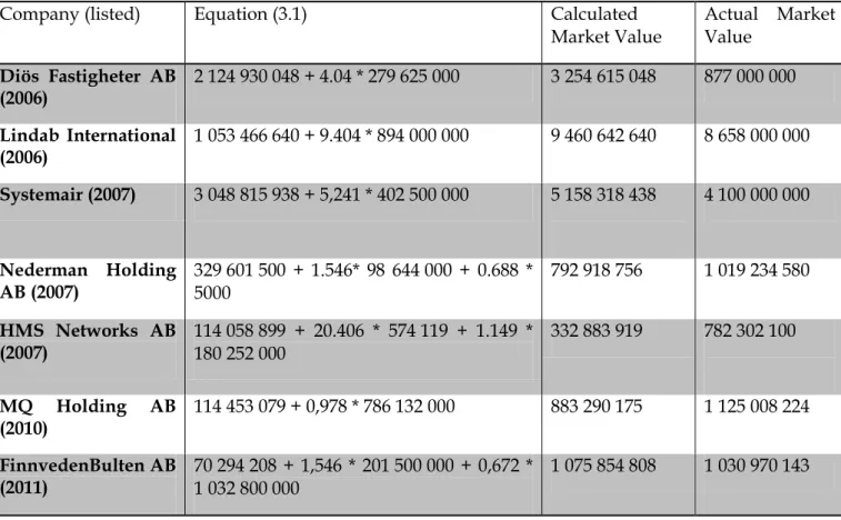
Table 12. Overview of calculated and actual market values ... 30
Appendix 1. ... 42
Appendix 2. ... 48
Appendix 3. ... 57
Appendix 4. ... 58
1
1 Introduction
The first chapter will give the reader an introduction to the subject of the thesis. Background information will introduce the reader to the problem discussion and furthermore to the pur-pose intended to be fulfilled throughout the research.
1.1 Background
In order to make wiser business decisions, a stakeholder of a company uses information often related to the value of the company. However, the process of valuing a business is not an easy one. The main reason being that in order to know what a company is worth today one must also know where it is headed in the future. There is an uncertainty that lies in the techniques utilized today that concerns the forecasting of the remaining life expectancy (Hult, 1998). Defining a value for a business is of interest in several situations and for several stakeholders. The value determines the price in the case of a takeover or a disposal but is also needed dur-ing mergers, capital investment, initial public offerdur-ings or credit processes. In each one of these cases it is evident that private persons as well as managers, investors and financial insti-tutes are interested in the valuation of a business (Hult, 1998).
Over the last decade financial markets have experienced periods of major booms and reces-sions, displaying that companies’ market values, which are heavily affected by the economy itself, can change rapidly. The importance of having knowledge regarding companies’ market values and what factors are value drivers has increased, not only for controlling parties in the company but also from an accounting, financing and business leader perspective (Pwc, 2007). A company is considered to be listed, i.e. public, if its shares are admitted to trading on a reg-ulated market. The valuation of an unlisted company is in general a more difficult task than the valuation of a public company due to the lack of a noted price as a reference. According to Nilsson, Isaksson & Martikainen (2006) the selling price of companies with similar character-istics can be used as an indication for determining the value of unlisted firms. However, these prices are often, if even existing, confidential information and one might face difficulties try-ing to find perfectly comparable companies. In most international macroeconomic statistical manuals, market prices are regarded as the most suitable valuation principle of assets accord-ing to International Monetary Fund (IMF) (2009). Such a method is straightforward when handling regularly traded assets in the markets, but more complicated for unlisted equity as market prices are not readily available. Since such prices cannot be directly observed,
estima-2
tions have to be made in its place (IMF, Balance of Payments and International Investment Position Manual, 6th ed. (BPM6), 2009).
Depending on how appraised stock prices differ from market prices, estimations can be more or less reliable. Since information is not equally available for all assets, International Ac-counting Standards Board (IASB) developed the acAc-counting guidelines IFRS 13 with the con-cept of fair value hierarchy. Firstly an assessment is made in order to establish how much in-formation that can be observed regarding prices and, thereafter the most appropriate level for fair value estimations is chosen. The structure is split into three parts ranging from 1-3, with the same priority. Level 1 entails quoted prices in active markets for identical assets or liabili-ties. Depending on how much is traded on the specific asset, the fair value is achieved by tak-ing the product of the quoted price and the quantity traded. Level 2 consists of inputs that can be found either directly (prices) or indirectly (derived from prices). Level 3 corresponds to unobservable inputs. Such inputs should be developed using market participant assumptions (Larsen, Nunes, Palmer, Garey & Todorova, 2011). Regardless of which level is chosen for fair value approximations, such level should be applied consistently (Ernst & Young, 2011). The purpose of valuing an unlisted company is often the determinant for how such valuation is conducted in terms of the magnitude and direction of the analysis as well as what method-ology is utilized. Furthermore, the purpose is also the basis for what definition of value that should be the starting point for the valuation. Since a valuation is of subjective nature, it is of high importance to have knowledge of why the valuation is made as well as who is principal (PwC, 2007).
1.2 Problem Discussion
When actual market values with an adjustment for movements in share prices and exchange rates are not available, the task of determining value of equity is a complicated one. As has been said before, defining the value is of interest in several situations and for several stake-holders. However, there is an uncertainty that lies in the techniques utilized today and such is especially the case for unlisted equity. In light of this, the BPM6 manual serves as a standard framework for alternative methods of approximating market value of equity in unlisted com-panies. There are seven methods recommended for application by the BPM6; recent transac-tion price, net asset value, present value and price-to-earnings ratios, market capitalizatransac-tion method, own funds at book value and a portioning global value.
3
Kumah, Damgaard and Elkjaer (2009) have analyzed the seven valuation methods and tested generally applicable methods on Danish companies. The purpose of Kumah et al.’s study was to investigate to what extent the suggested methods produce both reliable and robust results for their dataset of Danish companies. Since models of relative nature1 are based on comparables, an important attribute in achieving reliable market value approximations is to ensure that such comparables are suitable. Reliability is a way for the compiler to test suitabil-ity and is referred to as the extent to which the techniques utilized produce consistent results (Saunders, Lewis & Thornhill, 2007).
Kumah et al. (2009) conclude that although the seven models put forward in the BPM6 pro-vide enhanced guidance there are still possibilities for diverse interpretations within each model. Furthermore, they suggest that in order for IMF to provide precise guidelines, similar studies should be conducted for other markets. In Sweden, no such extensive research has yet been conducted. This is why the authors wish to conclude if the models are appropriate for valuing unlisted equity in Sweden.
1.3 Purpose
The purpose of this thesis is to investigate the reliability of the suggested BPM6 valuation models, intended for listed companies, on unlisted equity in Sweden as suggested by Kumah et al. (2009).
After testing the suggested models the authors aim to conclude which model reflects the value of equity the best. That model is subsequently used in order to calculate a hypothetical market value. In order to test whether the hypothetical value is reliable, the unlisted equity chosen for this thesis will all have undergone an initial public offering, thus creating a possibility to compare the hypothetical value to an actual one. This research aims to fulfill an evaluative purpose as it aims to test the BPM6 methods on unlisted equity in Sweden.
1 For further description on the theory of relative models the reader is suggested to read section 2.1 Currently used Valuation Methods of this paper.
4
1.4 Delimitations
In the interest of focus, the study will concern Swedish companies that have undergone an IPO in the past six years. The reason for choosing this “timeframe” is due to the restriction of data availability. Searching for data prior to this period is aside from being time-consuming, a difficult task for a larger sample size.
In order to generate hypothetical market values for the dataset of unlisted equity, the calcula-tions will be made based on listed firms in the OMX Nordic Exchange Market. In order to ensure a large enough samples set the decision was made to include Danish and Finnish com-panies. This decision can be made on the basis of the ‘Nordic Model’ which economically implies that the Nordic countries have much in common. They are small and open economies that rely on foreign trade. Since they are also modern industrialized economies considered as competitive in the global market, it can be concluded that the Nordic countries face similar business potentials and risks (Norden, 2013).
5
2 Theoretical Framework
The purpose of chapter two is to present the basic theories as well as previous studies regard-ing the subject. The theories discussed will serve as a theoretical framework as it is intended to help the reader understand the empirical results and the analysis in the following chapters.
2.1 Currently used Valuation Methods
Theoretical models for valuing equity, both listed and unlisted, can be divided into two sub-groups; absolute and relative valuation models. Absolute valuation models aim at estimating a company’s fundamental value. In such valuation models firm-specific characteristics, e.g. dividends affect the value, meaning that the estimated value does not have to correspond with the market price. Depending on whether the assessments made regarding the business’ future earnings and risk are in line with market expectations or not, may result in potential differ-ences in value (Kumah et al., 2009).
Relative valuation models on the other hand, value a company based on comparables. The compiler identifies companies with identical or similar characteristics as reference. Due to arbitrage reasons, the asset which is valued must trade at similar prices as its comparables (Kumah et al., 2009). According to Hitchner (2006) relative valuation models are often uti-lized by compilers due to simplicity, data availability and use of comparable companies (cited in Kumah et al., 2009).
The Discounted Cash Flow (DCF) model and Relative Valuation model are the two most commonly used approaches when valuing companies2. They are often used simultaneously as they, once correctly used, should conclude the same results (PwC, 2007).
2.2 BPM6 Equity Valuation Models
The seven methods of approximating market value of equity suggested by the IMF are pre-sented in the following section. It is further suggested that these methods can be utilized for unlisted equity. Important to stress is that these are not ranked, implying that each model would need to be evaluated according to circumstances and the reliability of results (IMF, 2009).
2
The DCF model is explained in detail by Brealey, Myers & Allen (2006), Corporate Finance 8th ed and the Relative Valuation Method by PwC (2007), Företagsvärdering – översikt av området baserat på erfarenhet.
6
2.3 Models Included in this Study
2.3.1 Price to Earnings
According to this method, Price to earnings (P/E) ratios for listed companies can be calculated and applied to unlisted equity (Kumah et al. 2009). The P/E ratio is considered to be a form of relative valuation as the value of a company is determined based on available market values of other companies (Edenhammar & Thorell, 2009). The ratio is calculated for an entire com-pany as the accumulated value of the comcom-pany’s value divided by its earnings. A high ratio might indicate that the market believes in the prosperity of the company in the near future while a low ratio may indicate that the company is headed towards stagnation in the business cycle. The ratio is thus suggested to be used for companies within the same industries that can be expected to have the same prospects and are at the same stage in the business cycles (Edenhammar et al. 2009). With consideration to this, Kumah et al. (2009) recommend that the ratios should be calculated for industry groups in order to estimate across similar compa-nies rather than calculating a common P/E ratio to be applied to all compacompa-nies within that industry group.
This method is fairly easy to implement and also uses actual market values rather than predic-tions such as expected earnings and interest rates which serve as clear advantages. A disad-vantage is that it does not take individual company characteristics into account e.g. if a certain company is expected to prosper faster in the future than its peers, such effect will not be taken into account by the P/E model. The assumption that a model based on listed equity can be transferred to unlisted equity is also made in this model; this will be discussed more in depth in section 2.8 Transferability.
2.3.2 Price to Book Value
The price to book (P/B) value method is of a relative nature, implying that comparables are used in order to approximate the market value of a firm’s equity. The method is considered as a market capitalization method where compilers adjust companies’ book values at an aggre-gate level. The BPM6 manual argues that book value do not necessarily estimate market val-ues well and therefore puts forward the concept of Own Funds at Book Value (OFBV). When approximating OFBV, data is gathered from companies and subsequently adjusted with ap-propriate ratios. A suitable example is the ratio of market capitalization to book value for listed companies within the same industry and with similar operations. An alternative way of
7
estimating OFBV is to revalue assets that contain costs for the company at current period prices, using appropriate indices (IMF, 2009). The implementation of the price to book value method requires applying a calculated P/B ratio generated from a peer group of listed compa-nies to a specific unlisted company.
Essentially, the price to book value method possesses the same advantages and disadvantages as the relative price to earnings method. There are however some differences for certain sce-narios where one model may be superior to the other. The present value of earnings are often-times regarded as the general theory of equity valuation, implying that it may, on the face of it, seem more attractive to use earnings as input rather than book value. For cases in which earnings are highly volatile or negative, book values may be more suitable to use as input in the sense that such values tend to be more stable. Furthermore, book values do to some degree include earnings as well as the accumulated earnings of previous years’. It is important to point out however that no method can be regarded as being better than the other (Kumah et al., 2009).
2.3.3 Own Funds at Book Value (OFBV)
The own funds at book value (OFBV) method for valuing equity is of absolute nature. The purpose with this method is an attempt to standardize the term book value since it diverges across countries. According to the IMF, this model for valuing equity is “the value of the
en-terprise recorded in the books of the direct investment enen-terprise, as the sum of (a) paid-up capital (excluding any shares on issue that the enterprise holds in itself and including share premium accounts; (b) all types of reserves identified as equity in the enterprise’s balance sheet (including investment grants when accounting guidelines consider them company re-serves); (c) cumulated reinvestment earnings; and (d) holding gains or losses included in own funds in the accounts, whether as revaluation reserves or profit or loss.” Emphasize is put on
frequent revaluations of asset and liabilities as the higher the frequency of revaluations the closer the estimation to market values. By the same token, market value approximations tend to be poor in terms of reflecting the true value when handling data that has not been revaluat-ed for several years (Kumah et al., 2009).
The OFBV method for valuing equity has two main advantages, namely that the method is relatively easy to utilize and, if implemented by all countries would promote homogeneity in recording. Nevertheless, the method also has disadvantages. Even though actions have been
8
taken by IASB in order to estimate market values, differences still appear between valuations. Such differences are especially noteworthy in terms of handling intangible assets, which may be a major element of a company’s market value. Kumah et al. (2009) state that book values might undervalue market values in the sense that several intangible assets are eliminated from the IFRS. Conversely, overestimates may also be a possibility within the OFBV method as experiences have shown that book values are only written down after a certain loss has been sustained. Both these scenarios lead to book values not reflecting market values correctly. A further drawback this equity valuation method possesses is that the IFRS regulations are not fully implemented in all countries meaning that accounting standards still differ (Kumah et al., 2009).
2.4 Models Excluded from this Study
2.4.1 Recent Transaction Price
Recent prices for a maximum of a year back, at which unlisted instruments were traded, may be used as an estimate as long as there has been no material change in the company’s position since the transaction date. To the extent that market conditions from when the trade was con-ducted are unchanged, the recent price serves as a good indicator of current market values. However, recent transaction prices become increasingly misleading as time passes and condi-tions change. Furthermore this method cannot be implemented in case the company has initi-ated corporate actions such as large dividends or stock splits since the transaction date (IMF, 2009).
2.4.2 Net Asset Value
The net asset value method targets first-hand information from knowledgeable insiders of a business, such as the management or independent auditors. The aim is to obtain total assets at current value deducted by liabilities at the market value in order to make assessments of un-traded equity. The requirement is that valuations need to be conducted within the past year and should preferably contain intangible assets. Since first-hand information is required for the net asset valuation technique it is evident that insiders, who most often have superior knowledge about the specific company, generate such information (IMF, 2009).
9 2.4.3 Present Value of Earnings
To calculate the present value or the fundamental value of a company, expected future earn-ings can be discounted. This method requires the prediction of future earnearn-ings and the deter-mination of an appropriate discount rate with consideration to risk factors. However, it is time-consuming to make reliable earnings forecasts, if even possible at all, at a company level (Kumah et al. 2009).
2.4.4 Apportioning Global Value
IMF states that the current market value of each of the companies in a listed global enterprise group can be based on the market price of its shares on the exchange on which its equity is traded, if it is a listed company. Sales, net income, assets or employment figures can be used as apportioning indicators (Kumah et al., 2009).
2.5 Argumentation for delimitation of Models
Despite the seven suggested models put forward in the BPM6 manual, four of these models are unfeasible for this study due to the limitation of data. The secluded models are not based on common publicly available data, such as price, earnings, and book values.
The argument for the ability to use common publicly available data rules out the method of recent transaction price as, while this method might be easy to implement, it requires that a recent transaction price exists which is rarely the case for unlisted equity. This is also why apportioning global value cannot be used, as many unlisted companies are not a part of a listed group. Moreover, in order to avoid the potential of bilateral asymmetries that arise from subjective assumptions about a company or its future expected earnings the present value of earnings method has been ruled out. For the very same reason, the net asset value method has been eliminated as it requires the compiler to have access to inside or first-hand information about a company.
It should however be clarified that the ruled out models are not in any way inferior to the cho-sen models e.g. the recent transaction price. If such a price exists, it will often give the most accurate value equivalents for equity (Kumah et al., 2009). The choice of the models to in-clude is thus simply based on practical reasons.
10
2.6 Previous Research
Ohlson (1995) puts forward in his framework the clean surplus relation i.e. that the change in book value must equal earnings minus dividends. The purpose of the Ohlson framework is to investigate if one can develop a solid theory of a company’s value that relies on the clean sur-plus relation in order to identify a distinctive role for the following variables – earnings, book value and dividends. Overall, Ohlson’s framework contributes as a benchmark model, to the accounting literature, that relates a company’s market value to the accounting/information variables stated above. The main assumption that this theory relies on is the clean surplus re-lation as well as the feature that dividends reduce book value but leave current earnings unaf-fected. According to Peasnell (1981), the present value of expected dividends and the clean surplus relation indicate that a company’s market value equals the book value plus the present value of future expected abnormal earnings. This implication allows for the valuation analysis to disregard dividends and focus on the prediction of abnormal earnings. The primary value indicators are thus composed by earnings and book values. Specifically, the core of the valua-tion funcvalua-tion expresses market value as the weighted average of (i) capitalized current earn-ings and (ii) current book value.
The importance of including earnings is also stressed by Kantor & Pike (1987) that claims that earnings prospects is the single most important factor in the determination of the value of unlisted equity. Beaver (1981) points out that under the assumption of perfect market condi-tions, earnings and value are really two sides of the same coin (cited in Kantor & Pike, 1987).
2.7 Issues with Valuing Equity
According to Kumah et al. (2009) there are three main complications, two of which are topi-cal for this thesis, when valuing equity. The complications, (i) liquidity and (ii) the value of control, apply to both absolute as well as to relative valuation methods.
The liquidity of an asset deals with the trading costs associated with the trading of such asset. Stocks that belong to unlisted companies are significantly harder to value and is therefore not as easily marketable i.e. they are considered to be illiquid. (Bodie, Kane & Marcus, 2009). “The cost of illiquidity” consists of three components; the bid-ask spread, the price impact when trading and the opportunity cost of waiting (Damodaran, 2005).
11
The first component i.e. the bid-ask spread refers to the difference between the bid price and the ask price. Depending on the degree of liquidity of an asset, the size of the bid-ask price tends to vary. If an investor aims to trade a highly liquid asset the spread tends to be insignifi-cant in the sense that the buyer and seller generally agree upon the appropriate price.
The price impact component of the illiquidity cost refers to the impact that a trader can create by trading on an asset, by pushing the price up when buying the asset and pushing it down while selling. This impact can be explained by an informational factor e.g. an investor that buys a large block of the asset signals good news about the company to other investors while selling a large block indicates negative news – indirectly this affects the attitude towards the asset that investors have and consequently pushes the price.
The third component is the opportunity cost of waiting. In theory, an investor could reduce the bid-ask spread and the price impact costs of trading by trading the asset over a longer period of time. However, there is a cost of waiting e.g. the price of an asset that the investor wants to buy (sell) because he or she believes that it is undervalued (overvalued) may rise while the investor waits to trade which in turn can lead to reduced expected profit for the investor. The probability that the investor assigns that the price will rise (fall) while he or she waits to buy (sell) thus affects the cost of waiting to a great extent (Damodaran, 2005).
The second complication, value of control also has a significant impact when valuing equity. Unlisted companies often have either one single investor or very few owners. When investors acquire a controlling share in a company, a control premium is often included since investors believe they can increase the value of the company through efficiency gains. If a controlling portion of a private firm is offered for sale, this particular portion should have a substantially higher value than if it is a non-controlling share. However, the estimation of how much the value of control is worth is a difficult task (Damodaran, 2005).
Pratt, Reilly & Schweis (2000) distinguish the value of the controlling and the non-controlling share of a business by allocating different terms for the two situations. An asset’s lack of
mar-ketability concerns the inability of the owner of a non-controlling equity share to convert his
or her investment to cash quickly and at a reasonably low and predictable price. Illiquidity refers to the owner of the entire business enterprise i.e. the controlling party, and his or her ability to convert the investment into cash.
12
2.8 Transferability
Relative equity valuation models intended for listed equity rely on four assumptions in order to be regarded as suitable valuation models for unlisted equity. If not fulfilled, such models would not be satisfying in the sense that estimations are likely to be incorrect and hence not be appropriate to use for valuation. The four assumptions are the law of one price (LOOP), existence of comparables, transferability of the model and projections outside the data range (Kumah et al., 2009).
The first assumption is that in capital markets, LOOP implies that identical securities should trade at identical prices. In general it is expected that LOOP holds in the long run restoring a potential arbitrage situation (Lamont & Thaler, 2003). The assumption of LOOP is likely to hold for the Nordic market as there are a large number of active investors on the market and due to lack of capital restrictions.
The second assumption is the possibility to find comparables when performing a relative val-uation model for unlisted equity. Eberhart (2001) concludes through investigations that the greater the similarity between the comparables and the firm being valued, the better compara-bility, implying that more information is generated. When identifying suitable comparables, the compiler needs to locate companies with identical multiples in order to have a virtuous peer group. Even though identical multiples are not generated and the independent variables do not fully explain all variation in market values, compilers may be able to utilize a model as long as there are no systematic differences, such as liquidity, between listed and unlisted companies (Kumah et al., 2009).
The implication of the third assumption, transferability of the model, refers to if models intui-tively intended for listed companies can be successfully transferred and utilized for unlisted companies. Transferability is achieved by satisfying three main criteria. Firstly, assessments regarding future risks and potential earnings need to be identical for listed and unlisted com-panies. This criteria would be a concern in the case that only listed companies were able to get lucrative contracts in certain business areas, which is not the case on the Nordic market. Fur-thermore the potential differences in risk are embedded in earnings or other accounting varia-bles rather than in the business environment (Kumah et al., 2009). Secondly, the listed and unlisted companies must have similar capital structures implying that the two types of compa-nies face the same optimization problem of deciding the financial leverage ratio. Kumah et al.
13
(2009) state that when tax rates do not differ between listed and unlisted companies the com-piler can conclude that the financial leverage ratios are in fact identical. The third implication refers to homogeneity in accounting regulations. For transferability, such accounting regula-tions should not result in systematic differences in accounting data between the listed and unlisted companies (Kumah et al., 2009). The general criteria to adopt IFRS standards in ac-counting, concerns all listed companies within OMX Nordic Exchange Market (Deloitte, 2013) and therefore can be said to be consentient regarding financial reporting.
The final assumption states that it should be possible to create realistic assessments regarding enterprises not included in the input data. Such projections can refer to factors such as liquidi-ty, the reason being that unlisted companies tend to be less liquid than otherwise similar listed companies (Kumah et al., 2009).
14
3
Method
In this chapter the authors will describe the research approach that has been applied in this thesis. The reader will also be provided with an insight in which research technique that has been used. Lastly, the data collection and research process will be explained.
3.1 Research Approach
According to Saunders et al. (2007) method is the procedures and techniques used to obtain and analyze data. Since this thesis aims to investigate the reliability of equity valuation mod-els, put forward in the BPM6 manual, the deductive research approach is appropriate. Such approach starts with the collection of previous studies before forming a hypothesis regarding a certain relationship between two or more variables. In order to test such hypothesis, collection of data is necessary, most often conducted in a quantitative manner. As the aim with this the-sis is to make inferences regarding the reliability of valuation models, done by testing the sig-nificance on quantitative variables, data concerning earnings, volume, OFBV and EBIT will be collected. This thesis will thus process the quantitative information with the help of statis-tics, enabling the examinations of relationships between variables.
In order to be able to fulfill the objectives of a study one should utilize exploratory, descrip-tive or explanatory studies. Explanatory studies put emphasize on investigating a situation or a problem in order to establish causal relationships between variables, often made in terms of quantitative data gathering. Once the data is collected one can subject it to statistical tests in line with what the aim with the test is in order to get a clarified view of the relationship (Saunders et al. 2007).
3.2 Research Technique
For the objective of testing the reliability of equity valuation models to unlisted equity, the authors have chosen to use a combination of a quantitative event study and a statistical meth-od. The use of financial market data in an event study can measure the impact of a specific event on the value of a firm according to MacKinlay (1997). Given rationality in the market-place, the benefit from an event study stems from the fact that the effects of an event will im-mediately be reflected in security prices. Hence, the measure of an event’s economic impact can be constructed by observing significant variables over a certain time period. For the ob-jective of this particular thesis the statistical method will be used in order to analyze the col-lected data. The events that will be studied relate to each company’s financial variables
ob-15
served in the event of an IPO. These events will serve as a basis for deciding whether the hy-pothetical value generated from the statistical method is reliable or not.
3.3 Credibility
In order to reduce the possibility of incorrect answers, attention has to be paid on the credibil-ity of research findings i.e. to put emphasize on reliabilcredibil-ity and validcredibil-ity (Saunders et al., 2007).
3.3.1 Reliability
The extent to which the chosen data collection techniques and analysis procedures will yield consistent findings is referred to as reliability. Easterby-Smith, Thorpe & Lowe (2002) sug-gest that in order to assess the reliability factor the following three questions should be posted:
1. Will the measures yield the same results on other occasions? 2. Will similar observations be reached by other observers?
3. Is there transparency in how sense was made from the raw data?
Robson (2002) argues that there may be four threats to reliability, some of which apply to this thesis as well. Subject and participant error implies that various results are achieved at differ-ent times, which will be controlled by the fact that the authors have divided the data into both industry categories as well as years, taking business cycles into account. The possibility of misreading the observed financial reports is also a factor that is a threat to reliability, referred to as observer error. The room for error however is fairly small since the data has been col-lected manually for every company in the respective peer groups and not through a data base.
3.3.2 Validity
Validity refers to whether the findings are concerned with what they appear to be about or not i.e. if the relationship between the variables is a causal relationship or not. Causal relationship refers to a relationship between variables in which the change in one variable is a result of the other variable(s) (Saunders et al., 2007). It is reasonable to believe that the independent varia-bles will be causally related in the sense that higher earnings and EBIT will cause a higher OFBV the forthcoming years.
3.4 Data Collection
Information concerning IPOs is chosen as benchmark values in order to determine the reliabil-ity of the equreliabil-ity valuation models. Statistics regarding which Swedish companies that have
16
become public between the years 2006-2012 is provided by NASDAQ OMX. The total num-ber of IPOs during this period creates a population of 26 companies. The year 2009 however has been secluded from this study as no IPO’s were conducted that year. Due to restrictions generated by insufficient peer groups and changed circumstances e.g. companies no longer listed on OMX Nordic, 13 of these were secluded from this study and the remaining were sorted based on industry classifications. However, as the regression models were conducted, five companies had to be excluded as the variables included in those demonstrated
multicollinearity and negative goodness-of-fit measures3. Thus, the final data set of unlisted
companies consists of eight companies.
The financial data has been collected from every company’s annual report retrieved from each company’s webpage. According to NASDAQ, all public financial information from the past three years of a company must be publicly available on the webpage. Furthermore, financial reports since at least five years back must be available on the webpage. It is also a criterion that the financial reporting of listed firms is substantially harmonized across stock markets in Stockholm, Helsinki and Copenhagen in order to simplify information for investors (Directive on Markets in Financial Instruments, Mifid 2004/39/EC). The decision is made to include those companies that went public between 2006 and 2012 in the sample as it is simpler to find the needed financial information for this time range, due to the legal requirements stated above. It is important to keep in mind that the companies work with different fiscal years for their annual reports e.g. Denmark divides their fiscal years into the second half of one year combined with the first half of the following year. This is also the case for some of the Swe-dish companies and hence there may be a possibility of subject and participant error (see sec-tion 3.3.1 Reliability).
In order to categorize the listed companies in reliable peer groups a detailed industry classifi-cation system is utilized. This is mainly due to the fact that the financial variables chosen for testing the valuation models e.g. potential earnings and risk most likely differs across various industries (Kumah et al., 2009). The GICS structure consists of 10 sectors, shown in Table 1, and these are the classifications that are used for the purpose of this study.
3 The reader is referred to section 3.7 Analyzing the data for further information regarding multicollinearity
17
Each of the investigated IPOs used in this study are classified according to the GICS struc-ture. Thereafter peer groups within the same corresponding GICS sector are selected from NASDAQ OMX. NASDAQ also uses the GICS classification system for listed companies which provides homogeneity in the classification approach.
In order to generate reliable estimates the data sample needs to be rather large, thus the peer groups in this study includes all listed companies on the Nordic Exchange Market. Although the valuation model will only be applied to Swedish companies, the Swedish stock market at the sector group level is of limited quantity. By including data from the entire Nordic ex-change market, estimations will be based on a larger number of observations. According to Kumah et al. (2009) the Nordic market is overall similar to the Swedish market and provides comparable business potentials and risks. Since the peer groups are based on the Nordic mar-ket, this implies that the financial statements collected are based on different currencies. As the unlisted companies are solely Swedish, the decision is made to convert the financial varia-bles into Swedish Kronor (SEK). The year-end exchange rates used are gathered from
Riksbanken for each observed year (2013).
For each of the years, firms listed after the year of the observed IPO are secluded as it is not a valid case to study for that particular IPO. For this purpose, information is collected from Avanza bank about the time of IPOs of the listed firms within each peer group. For further
Table 1. GICS Industry Classifications
Sector Sector Code Energy 10 Materials 15 Industrials 20 Consumer Discretionary 25 Consumer Staples 30 Health Care 35 Financials 40 Information Technology 45 Telecommunication 50 Utilities 55
18
segmentation, the peer groups are divided into mid- and small-cap in order to remove the scale effects likely to distort calculations. A company is put into different segments depending on its size of market capitalization. Companies with a market value smaller than EUR 150 million belong to the Small Cap segment whereas companies with a market value between EUR 150 million and EUR 1 billion belong to the Mid Cap segment (NASDAQ OMX, 2011). Kumah et al.’s (2009) paper serves as a point of departure for this study and, therefore similar variables are included in this study as well for the purpose of testing the BPM6 models. The variables included in the research are presented in Table 2:
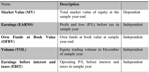
Table 2. Variables included in Regression analysis
Name Description
Market Value (MV) Total market value of equity at the sample year-end
Dependent
Earnings (EARNS) Profit and loss (P/L) before tax in sample year
Independent
Own Funds at Book Value (OFBV)
Own funds at book value at sample year-end
Independent
Volume (VOL) Equity trading volume in December
of sample year
Independent
Earnings before interest and taxes (EBIT)
Operating P/L before interest and taxes in sample year
Independent
Market value is the general valuation principle and is therefore an appropriate measure for equity valuation. The earnings measure chosen for investigation is the P/L before tax. The decision to include such measure is due to the listed companies included in the data set are operating in various countries. By taking the earnings before tax, the effect of possible differ-ences in such rates is excluded.
EBIT has been included as an alternative earnings measure in order to cross-check whether financial items, e.g. interest incomes and costs, generate additional information in terms of explaining market values or not. In the EBIT measure, financial items are not accounted for unlike P/L before tax. By performing a cross-check, the authors can ensure that results gained are not subject to a consequence of a more or less precise definition of earnings measure.
19
Specifically, it is argued in the BPM6 manual that OFBV is an appropriate measure of book value. When observing annual reports it is noticed that the majority of companies in the data set have the same design of reporting equity figures, which is equivalent to the definition of OFBV. Therefore, the choice is made to include the total equity that is attributable to parent company shareholders.
A trading volume variable is included in the research by the fact that liquidity is likely to in-fluence market values (Kumah et al., 2009). Furthermore, illiquid investments are likely to trade at lower prices compared to liquid investments and thus generate higher return (Damodaran 2005). The statement empowers the argument for including a trading variable. The reason for why December was chosen for every year observed was largely due to it being the closest to the end of period when the financial statement is compiled, generating the most reliable result.
3.5 Model Analysis
In this study, a multiple regression model is used to describe the relationship between selected financial data and the market value of equity. By finding the relationship, this model will help determine what variables are of importance when estimating market value and subsequently which one of the recommended valuation techniques put forward in the BPM6 manual gener-ate the most reliable results. The equation that provides the relationship between k independ-ent variables and the dependindepend-ent variable is (Donnelly, 2013);
Where represents a regression coefficient that predicts the change in a dependent variable
due to a one-unit increase in an independent variable while the other variables are held con-stant, represents the y-intercept of the regression line and is an error term for capturing randomness. This study will, by identifying the values for and all , predict the market value of equity which is denoted as . The rule of thumb concerning the number of observa-tions for each independent variable is 10-20 (Harrell, 2001).
Five different combinations of the independent variables are chosen, similar to Kumah et al’s (2009) research. The first model includes earnings and the liquidity variable volume and can be regarded as an alternate method of the P/E valuation method. The second model includes OFBV and volume and can be regarded as a variant of the P/B valuation method. The third
20
model includes earnings, OFBV and volume as independent variables, as suggested by the Ohlson (1995) framework in section 2.6 Previous Research. In order to determine whether or not financial items have an impact on the reliability of the chosen model, the independent variable EBIT is included instead of earnings for the fourth and fifth model. The fourth mod-el, similar to the first modmod-el, is regarded as an alternative method the P/E valuation method. Table 3 describes the regression models used as equations where represents the constant,
represents the coefficients and represents the error term, reflecting randomness.
The research is conducted in two steps. Firstly, the independent variables of the listed compa-nies in the respective industry groupings and years are regressed against the dependent varia-ble, market value. The specific models for each year and industry are run in order to match the unlisted company the best i.e. to locate the most successful fit. This in order to test which combination of variables does the best job in explaining market values. Thereafter, the gener-ated parameters from the regression that show the best fit are used in order to calculate a hy-pothetical market value of the unlisted companies in each year and industry. In the second step of the research, the hypothetical market value is compared to the initial public offering price. The IPO value is collected from each company’s prospectus and determined by the
Table 3. Possible Regression Models on Market Value of Equity
Regression 1 – Earnings model on market value of equity
Regression 2 – OFBV model on market value of equity
Regression 3 – Multi-factor model on market value of equity
Regression 4 – EBIT model on market value of equity
Regression 5 – Multi-factor model on market value of equity
21
number of shares multiplied by the introduction price. By performing this study, a conclusion is made regarding the reliability of the put forward equity valuation model.
3.6 Hypotheses Testing
Hypothesis testing is used in order to test an assumption, in this case that the independent var-iables (earnings, EBIT, volume and OFBV) affect market value. In order to see whether the coefficients included in each regression model have an effect on market value as a whole, i.e. to test the overall significance of the model, done by examining the F-value, the following statement is examined;
: All : At least one
The null hypothesis assumes that no relationship exists between the dependent and independ-ent variables i.e. that earnings, EBIT, volume and OFBV do not explain market value on a statistically significant level. Rejecting the null hypothesis provides support that a relationship exists between the variables and that it is appropriate to use such model for determining mar-ket value.
Subsequently, the following hypothesis statement will test whether the specific independent variable (earnings, EBIT, volume and OFBV) have an impact on market value or not;
: :
Where i represents the individual variable used for the regression model. If the null hypothesis is rejected one can conclude that the independent variable has an impact on market value.
3.7 Analyzing the data
In order to check for validity, the choice of using the coefficients of determination ( ) was made as an initial test. For a standard linear regression is used as a goodness-of-fit meas-ure (Cameron & Windmeijer, 1997). Adding additional independent variables to a regression model will increase the value of . Since this study involves several independent variables, the adjusted ( ) will serve as a better tool to help determine which regression model does the best job in predicting market value. The adjusted ( ) adjusts the goodness-of-fit measure by
22
accounting for the number of independent variables as well as the sample size. Since the ad-justed ( ) indicates to what extent the model explains market value in percentage, a higher measure corresponds to a better model. After the choice of model, based on the highest ad-justed ( ), the additional factors that will be examined further are; variance inflation factor (VIF), F-value, p-value and graphical interpretations.
Independent variables that are highly correlated with each other can cause problems for the multiple regression model (Donnelly, 2013) this is referred to as multicollinearity. The pres-ence of multicollinearity is detected by the variance inflation factor (VIF). According to Don-nelly (2013) if any of VIF exceeds 5.0 enough correlation exists between the independent variables to claim that multicollinearity is present in the regression model.
To test the overall significance of the regression equation, the first hypothesis statement will be examined. The critical F-score, , will be used as a reference point to see whether the re-gression model can be used to determine the market value of equity. The critical level as to which the F-value must exceed is obtained from the F-score table4. If it is the case that the F-test proves to be significant the next step will be to determine which independent variables belong in the final regression model by examining each variable separately.
The p-value states at what level each independent variable is significant for a predetermined confidence interval (Donnelly, 2013). If the p-value is less than the -value one rejects the null hypothesis and conclude that the relationship between that independent variable and mar-ket value is statistically significant.
In order to get a graphical interpretation of the statistical tests, inspections of probability plot
(P-P) of a regression standardized residual and a scatterplot will be observed as a part of the
analysis. Normality is demonstrated when the points in the P-P plot lie reasonably near the straight line that is graphed by Equation 3-1. The assessment regarding the scatter plot cerns observing if the points distributed around the zero point. If these points are roughly con-centrated along the zero-point, this implies there are no extreme outliers likely to distort the results.
4 The F-score table is found in most Business Statistics books. The reader is referred to Business Statistics
23 29% 15% 14% 14% 14% 14%
Industrials - Mid Cap Financials - Mid cap Industrials - Small Cap Information Tech - Small Cap
Cons. Discret - Small Cap Cons. Staples - Small Cap
Industry distribution of sample set
4
Empirical Results
Chapter four will present descriptive statistics and the empirical results generated from the test results. Such results will be described thoroughly in order to give the reader a clear in-sight of what they imply.
4.1 Characteristics of Data Sample
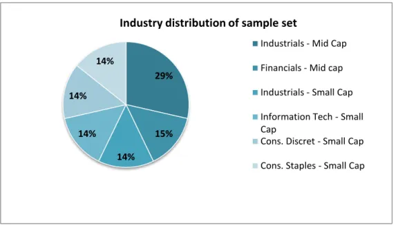
The final data set consisted of seven companies within six industries and sectors. The largest group and thus the most frequent occurring industry in the data set was ‘Industrials’, within the Mid Cap sector, representing 29 percent (see Figure 4-1). This can be partly explained by the fact that this industry had the most sufficient peer groups and therefore did not have to be secluded at any time. The IPOs that were removed from the data set had either insufficient peer groups making such groups too small to generate reliable results from, or that the com-pany was no longer listed on OMX Nordic.
Figure 4-1. Distribution of industries for the study
4.2 Summary of the Statistical Procedure
The empirical results presented in this chapter were collected through statistical analysis in the form of hypothesis testing, through regressions, of the collected data. The majority of the initial regression models had to be adjusted as the trading volume variable proved to be insig-nificant for most years and sectors. Since the aim with the regression models was to predict hypothetical market values for the unlisted companies, such insignificant variables, if includ-ed, would most likely have distorted the calculations. The initial factor considered when con-ducting the regressions was the adjusted , which proved to differ extensively between the
24
different regression model combinations, ranging from 0.9 percent to 90.6 percent. Overall, after having selected the best regression model for each industry and year, based on the ad-justed (see Appendix 3), the goodness-of-fit of such models proved to be above 50 per-cent. Only one sector, the ‘Consumer Discretionary’ industry within the Small Cap sector, showed a significantly lower goodness-of-fit measure (36.4 percent) compared to the other chosen regression models in the data set. The industry that showed the highest adjusted measure was ‘Industrials’ within the Small Cap sector with a measure of 90.6 percent. This was most likely due to the large sample of 72 listed companies within the peer group.
By performing regression models, the authors intuitively got a holistic perspective of the cho-sen regression models by examining the F statistic. Since the F-value proved to be statistically significant for all regression models, the authors therefore rejected the null hypothesis, imply-ing that at least one of the coefficients in the different regression models was significant when determining market value.
Overall, the VIF values for the regression models were all below five, implying that the inde-pendent variables were not correlated. Moreover, six of the regressions performed showed a VIF value of approximately one which is significantly below the critical value. Only one re-gression, the regression model performed on ‘Industrials’ within the Small Cap sector in 2007 showed a higher VIF value corresponding to 4.314. As this model included both earnings and book value measures, a higher VIF value is expected as stated in section 3.3.2 Validity.
Out of the five regression models, the combination with EBIT and volume (regression model 4) proved to be the most frequently used. However, as the volume variable proved to be in-significant for these models, they were remodeled to single regression models with EBIT as the only independent variable. Overall, the authors conclude that all five regression models proved to be best at least once for the different industries and years. For this study it can be concluded that the P/E valuation method is superior for predicting the dependent variable as it has been used for three out of seven sample sets in contrast to the multi-factor model and P/B model which were respectively used twice.
Graphical interpretations in the form of Normal P-Plots and Scatterplots were made and these can be found in Appendix 5. However, the sample sets were not large enough to make reason-able inferences from. This is why they have not been included in the analysis of data.
25
4.3 Results of Regression Models
4.3.1 Results for 2006
The tests for the data set of 2006 exceeded from a sample set of 50 companies where 28 were classified within the ‘Industrials’ sector and the remaining 22 in ‘Financials’ according to
Table 1. GICS Industry Classifications. Both of these industry groups are listed as Mid Cap
companies on OMX Nordic. For both industries, the best regression model proved to be mod-el 4 (adjusted R2 of approximately 76 percent for both industries) i.e. independent variables EBIT and volume (see Appendix 3). However in the case of industry ‘Financials’, the signifi-cance level for volume proved to be 0.907 and could therefore not be considered as statistical-ly significant on any level. Due to this reason, a new regression was made for ‘Financials’ with only EBIT (p-value of 0.000) included as the independent variable. The ‘Industrials’ sector proved however, to have a significance level for the volume variable right at the border line case (p-value of 0.137). The decision was made to exclude this variable for ‘Industrials’ as well as it sufficed better estimates for calculating market value. Table 4 and 5 provides an overview of the examined variables for each industry.
4.3.2 Results for 2007
For 2007, the sample set consisted of 175 companies sorted in three industries – ‘Financials’, ‘Industrials’ and ‘Information Technology’. The Mid Cap segment of ‘Financials,’ consisted
Table 4. Coefficients for ‘Financials’ Mid Cap 2006
Model b Sig. Adjusted R Square F-value
4 (Constant) 2124930046.643 .003 .761 67.956
EBIT 4.040 .000
Table 5. Coefficients for ‘Industrials’ Mid Cap 2006
Model b Sig. Adjusted R Square F-value
4 (Constant) 1053466640.172 .099 .746 80.273
26
of 29 companies, had to be secluded as the calculations showed that Volume was the only significant variable to explain market value which is not reliable. The Mid Cap segment of ‘Industrials’ also consisted of 29 companies but unlike ‘Financials’ generated more reliable results (see Table 6). The best regression model was, in accordance to previous year, model 4 (adjusted R2 of 53.4 percent) and the variable volume was also secluded (p-value of 0.913).
For ‘Industrials’ in the Small Cap sector, 72 companies were included and proved that regres-sion model 3, i.e. combining earnings and OFBV with volume, provided the best fit (adjusted R2 of 90.5 percent). However, when observing the p-values for each included variable it was noticed that volume was insignificant (p-value of 0.852) hence a new regression was made that excluded the volume as independent variable (see Table 7). The goodness-of-fit then in-creased to 90.6 percent and showed p-values of 0.000 (earnings) and 0.000 (OFBV). Even though, the model explains market value by almost 91 percent, the VIF was the largest out of all observations (4.314). As a VIF above 5 would indicate multicollinearity, this is not yet a problem although it is fairly close. This was the largest sample set to be tested which allowed for more reliable graphical interpretations than the others. As stated earlier in section 3.7
Ana-lyzing the data, the normal p-plot shows indications of normality. The pattern shows that there
are no major deviations from normality (see Appendix 5). The scatterplot shows that all ob-servations lie concentrated fairly close to zero as hoped for (see Appendix 5). This is also an opportunity to detect outliers. In this case it is evident that there exists one observation with extreme values. However, since it is only one no action needs to be taken.
Table 6. Coefficients for ‘Industrials’ Mid Cap 2007
Model b Sig. Adjusted R Square F-value
4 (Constant) 3048815937.508 .005 .534 33.149