V¨
aster˚
as, Sweden
Thesis for the Degree of Bachelor of Science in Computer Science
15.0 credits
HOW ACCURACY OF ESTIMATED
GLOTTAL FLOW WAVEFORMS
AFFECTS SPOOFED SPEECH
DETECTION PERFORMANCE
Johannes Deivard
jdd14001@student.mdh.se
Examiner: Ning Xiong
M¨
alardalen University, V¨
aster˚
as, Sweden
Supervisors: Miguel L´
eon Ortiz
M¨
alardalen University, V¨
aster˚
as, Sweden
Abstract
In the domain of automatic speaker verification, one of the challenges is to keep the malevolent people out of the system. One way to do this is to create algorithms that are supposed to detect spoofed speech. There are several types of spoofed speech and several ways to detect them, one of which is to look at the glottal flow waveform (GFW) of a speech signal. This waveform is often estimated using glottal inverse filtering (GIF), since, in order to create the ground truth GFW, special invasive equipment is required. To the author’s knowledge, no research has been done where the correlation of GFW accuracy and spoofed speech detection (SSD) performance is investigated. This thesis tries to find out if the aforementioned correlation exists or not. First, the performance of different GIF methods is evaluated, then simple SSD machine learning (ML) models are trained and evaluated based on their macro average precision. The ML models use different datasets composed of parametrized GFWs estimated with the GIF methods from the previous step. Results from the previous tasks are then combined in order to spot any correlations. The evaluations of the different GIF methods showed that they created GFWs of varying accuracy. The different machine learning models also showed varying performance depending on what type of dataset that was being used. However, when combining the results, no obvious correlations between GFW accuracy and SSD performance were detected. This suggests that the overall accuracy of a GFW is not a substantial factor in the performance of machine learning based SSD algorithms.
Table of Contents
1. Introduction 1
2. Background and related work 2
2.1. Automatic speaker verification systems . . . 2
2.2. Glottal flow . . . 2
2.3. Glottal inverse filtering . . . 2
2.4. Feature extraction and parametrization . . . 3
2.5. Aalto Aparat . . . 4
2.6. OPENGLOT . . . 4
2.7. Spoofed speech . . . 4
2.8. Automatic Speaker Verification Spoofing and Countermeasures Challenge . . . 4
2.9. Machine learning . . . 5
2.9..1 Artificial neural network . . . 6
2.9..2 Support vector machine . . . 6
2.9..3 Logistic regression . . . 6
3. Problem formulation 8 4. Method 9 5. Ethical and Societal Considerations 11 6. Implementation 12 6.1. Preprocessing OPENGLOT data . . . 12
6.2. glottal flow waveform (GFW) estimation and parametrization . . . 12
6.3. GIF method performance evaluation . . . 13
6.4. Machine learning classification . . . 16
6.4..1 Artificial neural network . . . 16
6.4..2 Support vector machine . . . 17
6.4..3 Logistic regression . . . 17
7. Results 18 7.1. glottal inverse filtering (GIF) method evaluation . . . 18
7.2. Machine learning models evaluation . . . 18
7.2..1 Neural network . . . 21
7.2..2 Support vector machine . . . 23
7.2..3 Logistic regression . . . 23
7.3. Combining the results . . . 23
8. Discussion 25 8.1. Limitations . . . 25
9. Conclusion 27
10.Future work 28
References 32
List of Figures
1 Illustration of the GFW estimation and parametrization step. . . 14
2 Illustration of the block-sampling process. . . 15
3 Grouped box plots of repository I sample score distributions. . . 19
4 Grouped box plots of repository IV sample score distributions. . . 20
5 Grouped bar chart displaying GIF method average scores on both parameter types. 21 A.1 Grouped bar charts displaying a side by side view of macro average precision of artificial neural network (ANN) models using Liljencrants-Fant (LF)-model domain parameter datasets and GIF evaluation scores. . . 33
A.2 Grouped bar charts displaying a side by side view of macro average precision of ANN models using time domain parameter datasets and GIF evaluation scores. . . 33
A.3 Grouped bar charts displaying a side by side view of macro average precision of support vector machine (SVM) models using LF-model domain parameter datasets and GIF evaluation scores. . . 34
A.4 Grouped bar charts displaying a side by side view of macro average precision of SVM models using time domain parameter datasets and GIF evaluation scores. . . 34
A.5 Grouped bar charts displaying a side by side view of macro average precision of logistic regression (LR) models using LF-model domain parameter datasets and GIF evaluation scores. . . 35
A.6 Grouped bar charts displaying a side by side view of macro average precision of LR models using time domain parameter datasets and GIF evaluation scores. . . 35
Acronyms
ANN artificial neural network AR auto-regressive
ASV automatic speaker verification DAP discrete all-pole
DWT discrete wavelet transform EGG electroglottograph
GFM-IAIF glottal flow model iterative adaptive inverse filtering GFW glottal flow waveform
GIF glottal inverse filtering GMM Gaussian mixture model HMM Hidden Markov Model
IAIF iterative adaptive inverse filtering LF Liljencrants-Fant
LPC linear prediction coefficients
LPCC linear prediction cepstral coefficients LR logistic regression
LSF line spectral frequencies
MFCC mel-frequency cepstral coefficients ML machine learning
MVDR minimum variance distortionless response NAQ normalized amplitude quotient
PLP perceptual linear prediction QCP quasi closed phase
QOQ quasi-open quotient SSD spoofed speech detection SVM support vector machine
1.
Introduction
Automatic speaker verification (ASV) systems uses a form of biometric recognition that utilize characteristics of the target speaker’s voice to verify the authenticity of the speaker. Biometric systems are usually designed to protect something from unauthorized users which implies that unauthorized users with ill intent exists and that they may attempt to fool the system to get access to the protected artefacts. Due to this fact, biometric systems must be secure and resist spoofing attempts and still be able to authorize the correct biometrics.
Speech synthesizer technologies are constantly improving and is a popular research area due to its many applications. The synthesizers have recently reached a level where they are almost on par with human speech [1]. It is obvious that if artificial speech are close to human level speech, ASV systems will have a hard time distinguishing between real and spoofed speech. So, the better the synthesizers get, the better the ASV systems must become at the task of spoofed speech detection (SSD).
Although much work has been done in the field of SSD, there is still much yet to be explored. Especially in the area of looking for small deviations in the characteristics of the GFW by using e.g. linear prediction residual, Teager Energy Operator profile and the variable length profile, as suggested by the authors of [2]. However, most GFW estimation techniques have not been compared to the ground truth waveform, since it is hard to measure the actual glottal flow due to the special equipment needed [3]. The authors of [4] performed a comparative study of GFW estimation techniques, but their work was heavily limited by the fact that the ground truth GFW for natural speech was hard to come by. OPENGLOT provides a dataset1 that contain speech
waveforms, both synthetic and natural, and the corresponding ground truth GFW that can be used to test the accuracy of GFW estimation techniques [3]. The comparative work for natural speech in [4] can now be expanded upon by using similar comparative methods to those that was used for synthetic speech, where the ground truth GFW was available. We do not know how the performance of the GFW estimation techniques affect the SSD algorithms that uses information derived from the GFW. With the help of the OPENGLOT dataset, the performance of the GFW estimation techniques can be evaluated more accurately, and in turn, the effect that the estimation technique’s accuracy have on SSD algorithms can be evaluated.
This report made an attempt in finding a correlation between the performance of GIF methods and SSD algorithms. The subject was a lot more complex than initially thought, which resulted in a conclusion that needs further work before it can be validated properly. The work done in this report can serve as a foundation for further studies in the fields as it identifies limitations and aspects in the field that can be further improved upon, such as availability of publicly available datasets that contain GFW samples and more detailed comparisons of GIF methods. The results presented in this thesis suggests that the accuracy of the GFW estimated by GIF method with varying accuracy does not affect the ability of machine learning (ML) based SSD algorithms to classify spoofed speech correctly. In addition to the suggested lack of correlation between GIF method performance and SSD algorithm performance, a high level evaluation metric is proposed for evaluation of GIF method overall performance.
The purpose of this report is primarily to spark interest in the SSD field, and in particular, spark further interest in investigation of information that can be found in the GFW. In addition to the interest this report hopes to create, it can serve as general outline for studies of similar kind by providing insight of the current limitations in the field and pitfalls of the approach taken in this report.
2.
Background and related work
Knowledge that is beneficial to the general understanding of the work done in this study will be presented in the following sections. Related work will also be presented for the topics in the field that are closest linked to the work done in this thesis.
2.1.
Automatic speaker verification systems
Biometric recognition aims to verify (authenticate) a supposed identity based on biometric infor-mation: biological and behavioral characteristics [5]. One form of biometric recognition is ASV, which uses the behavioral characteristics of the voice [5].
Before a voice can be verified in an ASV system, the waveform must be represented digitally, and the behavioral characteristics of the waveform used by the verification algorithm must be extracted. The first step usually involves recording speech via a microphone, which means that the waveform of the speech will degrade in quality by a varying amount depending on the quality of the microphone that is used. When a waveform degrades in quality it could mean that some characteristics of the waveform may have been lost, which in this case means that the ASV system have less information to work with. This makes the task of correctly verifying a claimed identity harder and fooling the system easier.
ASV systems are susceptible to several types of malicious attacks, where impersonation is one of them [6]. The goal of voice impersonation is to make a voice mimic another voice [7]. The process of voice impersonation, in the context of conversion and ASV, usually involves extracting style and characteristics of a target speaker and applying it to an adversary voice which aims to fool an ASV system. Several voice conversion techniques exist such as unit selection [8], Hidden Markov Model (HMM) [9], Gaussian mixture model (GMM) [10] and Non-negative matrix factorization [11]. The most recent state-of-the-art technologies use artificial neural networks [12], deep neural networks [1] and generative adversarial networks [13, 14] which have provided a big technological leap in this area.
2.2.
Glottal flow
During speech, air flows from the lungs through the windpipe and passes the vocal folds, that are responsible for producing voice [15]. The opening area between the vocal folds is called the glottis and the amount of air that passes through the glottis can be visualized with the help of an electroglottograph (EGG). The EGG measures the contact pressure between the vocal folds [16] and creates a GFW out of these measurements.
2.3.
Glottal inverse filtering
The glottal flow correlates to how voiced speech sounds and is thus voice characteristic information that can be used in speech transformation, as well as speech verification. However, the ground truth GFWs are cumbersome to create, and in most cases, it is not even possible to create them, since it requires special equipment. GIF refers to the methods that can be used on a speech recording to derive an estimation of the GFW [17]. Inverse filtering corresponds to cancelling the effects of the vocal tract in a speech waveform to estimate the glottal source [18]. The inverse filtering methods usually have an acoustic pressure waveform recorded by a microphone as input [19], but some inverse filtering methods use the oral flow signal obtained by a pneumographic mask [20]. GIF is conveniently used in studies that involve speech since it does not need any special equipment and can in many cases still produce an acceptable GFW.
A lot of different glottal flow extraction techniques have been suggested over the years. In [17], Alku performs an extensive review of GIF techniques and parameterization methods which are presented in chronological order over a span of five decades. The review shows that some of the earliest GIF techniques are still being used today [17]. Alku concluded, among other things, that the accuracy of GIF is hard to quantify and that several studies has shown that the estimation is especially unreliable when analyzing certain voice types. A prominent example of this is high-pitched speech. Another earlier study that reviewed glottal waveform analysis also concluded the difficulty of evaluating the glottal flow estimation [21].
This report will focus on comparing the performance of two GIF methods, namely: iterative adaptive inverse filtering (IAIF) [17], [19] and quasi closed phase (QCP) inverse filtering [22]. Where three variations of the IAIF method will be used, essentially craeting four different GIF methods. It is worth mentioning that GFW estimation methods are frequently being researched and new ways of estimating the glottal flow are still appearing. Glottal flow model iterative adaptive inverse filtering (GFM-IAIF) [23] is one of the more recent methods to estimate the glottal flow, which is an IAIF-based algorithm.
2.4.
Feature extraction and parametrization
Although the digital representation of speech is a prominent factor in speech verification process, it is not the only determining factor. Which characteristics, and how the system extracts them from the speech waveform is also a major determining factor.
Creating a parametric representation of a speech waveform can be done via various feature ex-traction algorithms. Several different methods for extracting different types of characteristics from speech waveforms exist. Some of the feature extraction techniques commonly used in speech recog-nition and identification are [24]: Mel-frequency cepstral coefficients (MFCC) [25], linear prediction coefficients (LPC) [26], linear prediction cepstral coefficients (LPCC) [27], line spectral frequencies (LSF) [28], discrete wavelet transform (DWT) [29] and perceptual linear prediction (PLP) [30]. The choice of feature extraction technique is dependant on the task at hand. Some features perform better with certain algorithms and some perform worse. An example of this is that both the authors of [31] and [32] found that LPC residual information could be effectively used with a GMM classifier to detect replay attacks.
In the domain of glottal flow, the most established parameterization model is the four parameter LF model [33]. The basic parameters included in the LF model are: EE, RG, RK and RA which are thoroughly described in: [33], [34] and [35]. In [36] the parameters are briefly explained as follows:
EE is the excitation strength, measured as the amplitude of the differentiated glottal flow at the main discontinuity of the pulse. The RA value is a measure that corresponds to the amount of residual airflow after the main excitation, prior to maximum glottal closure. RG is a measure of the glottal frequency, as determined by the opening branch of the glottal pulse, normalised to the fundamental frequency. RK is a measure of glottal pulse skew, defined by the relative durations of the opening and closing branches of the glottal pulse. [36]
In addition to the parameters included in the LF model, a lot of other ways to parameterize the glottal flow exist, such as the quasi-open quotient (QOQ) [37] and the normalized amplitude quotient (NAQ) [38]. Both QOQ and NAQ where used to evaluate the performance and behavior of GIF techniques in [4].
2.5.
Aalto Aparat
Aalto Aparat [39] is a free and publicly available tool that can be used for GIF and parametrization. This tool provides an easy way for researchers to analyze speech waveforms without having any prior knowledge to programming. The source code for the tool is also publicly available, which enables researchers with programming knowledge to adjust the tool to fit other needs.
A multitude of parameters extracted from estimated GFWs are provided by Aalto Aparat. The parameters are grouped into three groups: Time domain, frequency domain and LF-model. The details of all the parameters will not be explained here since it is not relevant for this particular study. If the reader is curious about the details of the parameters and how they are calculated, information can be found in the source code2 of Aalto Aparat (in the following files: glottal lf.m,
glottalfreqparams.m and glottaltimeparams.m).
2.6.
OPENGLOT
The authors of [3] recognised the issue that not many ground truth performance measurements existed on the current GIF techniques since the ground truth waveforms are cumbersome to pro-duce. To combat this, the authors created a publicly available evaluation platform that includes both synthesized speech (repository I-III) data and normal speech data (repository IV) and their corresponding ground truth GFW. Repository IV contain recordings of normal speech in the form of pressure signals measured by a free-field microphone and simultaneous GFW measured with an EGG.
2.7.
Spoofed speech
Spoofed speech refers to fake speech that aims to pass as real speech to some entity, usually in ASV systems. Spoofed speech can stem from several different sources. It can, among other sources, be obtained through voice conversion [40,41,14], speech synthesis [1] and replay of recorded speech [42], where replay attacks are one of the hardest spoofs to detect for an ASV [42].
2.8.
Automatic Speaker Verification Spoofing and Countermeasures
Chal-lenge
ASVspoof3 is an initiative that attempts to counter the vulnerabilities of ASV systems by
creat-ing SSD challenges that encourage individuals and organizations to engage in the research field. ASVspoof organizers have gathered data from various contributors and created a publicly available database with bona fide speech and fake speech generated with various algorithms. This database is meant to be used to test experimental SSD algorithms.
So far, ASVspoof have organized three challenges. The latest challenge was 2019 and the main objective of ASVspoof 2019 was to find countermeasures to spoofed speech attacks stemming from text-to-speech (synthesized), voice conversion and replay attacks [43]. To assess the performance of an SSD algorithm, ASVspoof 2019 participants were asked to use the tandem detection cost function (t-DFC) [44], which is a cost function specifically developed for the ASV domain [44]. The t-DFC metric is suitable for detailed evaluations on the performances of full fledged spoofed speech countermeasure algorithms.
2https://sourceforge.net/projects/aparat/ 3ASVspoof: www.asvspoof.org
2.9.
Machine learning
Machine learning (ML) is the collective term for computer based algorithms that iteratively tries come up with better and better solutions to a problem. This iterative process can be likened to the learning process in humans. ML is especially useful during research where predictions on large and complex datasets are involved [45]. A lot of ML algorithms have been developed lately, which makes the interest in the field as well as applications for ML algorithms increase.
Perhaps one of the most popular applications for ML algorithms is classification problems. The core of a classification problem is to attempt to predict which class that a data sample belongs to. This can be done by finding features that are characteristic for the different classes in a dataset, and then looking at the values of those features. Based on the values of the features in a sample, the algorithm can then make a prediction of which class that sample most likely belong to. A situation that ML practitioners can find themselves in when solving classification problems is having imbalanced datasets, where the occurrences of the classes in the dataset are varied. If these type of situations are not handled with care, it can result in a model that performs much worse than it should be. This can for example be shown when a trained model performs much worse on new data in the real world, than it did on the data during the training, or when a model is constantly miss-labeling the under-represented classes.
One way of dealing with imbalanced datasets is to use k-fold cross validation. This technique aims to give a better estimation of the prediction accuracy for a model than the estimated prediction accuracy without using the technique [46]. The outline of k-fold cross validation is to divide the training data into k equally sized sets, then train k models using each fold as validation data for one model while the other k−1 folds are being used as training data. The estimated prediction accuracy is then calculated by taking the mean accuracy for all models. The same order of operation can be applied for other evaluation metrics as well, not only accuracy.
The performance of a classification model can be evaluated by looking at several different met-rics. A standard evaluation metric is accuracy, which is simply the percentage of predictions that were correct. However, it is not necessarily the most useful metric, especially not for imbalanced datasets. For a binary classification problem with a dataset where the class balance is 99 to 1, a model could easily get 99% accuracy by classifying everything as the over-represented class. Hav-ing a model with 99% accuracy seems intuitively good, but with a class balance of 99 to 1, 99% accuracy is terrible. Choosing the right evaluation metric is important when determining how well a model performs, and it relies heavily on the situation at hand.
A performance metric that is suitable for imbalanced datasets, where all classes are equally as important to label correctly, is macro average precision. In binary classification were the two classes are positive and negative, the precision can be defined as: For all samples predicted as positive, how many of the predicted samples were actually positive. The equation for precision is as follows:
P = T P T P + F P
where TP is the number of true positive predictions and FP is the number of false positive predic-tions.
The precision can be calculated for the negative class as well by replacing TP with FP, and FP with TP in the equation above. In binary classification problems, the macro average precision metric describes how well the model performed on both classes with regard to the calculated precision for both classes. The equation for macro average precision is as follows:
Pavg=
P1+ P2
2
2.9..1 Artificial neural network
A popular type of ML algorithm for classification problems is the artificial neural networks (ANNs). These algorithms are roughly modeled like the neural structure of the brain, with neurons sending information to each others and automatically adjusting how strong the connection is between these neurons in a seemingly self-learning fashion [47].
Each neuron in a ANN support a few basic functions, similar to to those of real neurons in the brain. The artificial neuron takes in various inputs that are multiplied by connection weights, sums up the inputs, sends it through an activation function and finally passes it to the output paths that lead to other neurons [47]. The neurons in an ANN are located in different layers, most commonly structured as an input layer, one or more hidden layers and an output layer. Each layer can have different sizes and different activation functions. Some common activation functions for ANN binary classifiers are ReLU and Sigmoid. Their equations are as follows:
ReLU: f (x) = max(0, x) Sigmoid: f (x) = 1
1 + e−x
where x is the value in a neuron after all the weighted inputs for that neuron are summed. The output from the activation function will be the output for the neuron.
The performance of an ANN model is dependant on several different parameters that define the structure of the network. Some of important parameters are the amount of layers, how many neurons each layer has and which activation function each layer uses.
The optimal values for each of the parameters can be hard to find and can differ between different problems. Extensive research have been done in attempts to find optimal values for these parame-ters, especially regarding the amount of hidden layers and amount of neurons in each hidden layer [48]. Some common rule-of-thumb sizes to start with for hidden layers are i) 2/3 of the input layer neurons [49], ii) less than twice of the neurons in the input layer [50] or iii) between the size of the input layer size and the output layer size [51].
2.9..2 Support vector machine
One of the more math centered ML algorithms that can be used to solve classification problems is the support vector machine (SVM). The core function of an SVM is to find a hyperplane in which the different features of each class are being separated [52], and thus enable classification by looking at which sector a sample lies in.
Class separation can be easy for some classes with few features and can sometimes even be done visually by humans when the features are mapped onto a two-dimensional plane. When the features get more numerous, or they are scattered in a way that makes them hard to visually separate in a two- or three-dimensional plane, a more mathematical approach needs to be taken. The SVMs uses something called a kernel to translate features into higher dimensions, where the class-separating hyperplanes might be found. This is something known as the kernel trick [53]. Several different kernel functions can be used for the kernel trick, one of the simplest, but still a very useful kernel function, is the linear kernel. The linear kernel uses a linear function with a time complexity of O(N) [54], which enables fast training even when the feature sets are large.
2.9..3 Logistic regression
In addition to the two previously mentioned ML algorithms that are commonly used in classification problems we have logistic regression (LR). This technique can be used in traditional statistics, but
also as a machine learning algorithm due to its ability to learn. LR is commonly used in binary classification problems where the model, based on several input values, produces a probability between zero and one that a sample is the positive class [55]. If the probability is over 50%, the sample is labeled as positive, and if it is below 50%, the sample is labeled as the other, negative class. Even though it is most common to use LR for binary classification, it is also possible to solve multi-class classification problems with LR as well. In order to solve multi-class classification problems with LR, the multi-class problem needs to be reduced into multiple binary classification problems, where one model is trained for each binary classification problem. This is known as a one-versus-rest strategy. Each model is trained to accurately classify one of the classes as positive, and all the other classes as negative, then the predictions of all models can be combined to solve multi-class problems. However, these models needs to produce a confidence score of the labeling instead of just labeling in order to avoid ambiguity when the predictions from all models are combined to produce a final prediction.
The LR algorithm is based on a fitted logistic function that maps several input values to a single probability in the range of zero to one. The input values for the LR model can be either continuous data, discrete data or even a combination of both [55]. However, it is not necessarily the case that all the input values in a LR model are valuable for making accurate predictions. When computational power or time is a limiting factor, it can be wise to identify the significance of the different input values with the help of a Wald test [56].
3.
Problem formulation
The effectiveness of an SSD algorithm that utilize the GFW may depend on which GFW estimation method that is being used and which features that are extracted from the waveform. This is something that needs to be investigated further. Perhaps lower accuracy of the GIF does not present artifacts that appear in synthetic speech as well as GIF methods with higher accuracy does, and this may or may not affect the performance of the SSD algorithms. It is also possible that the accuracy of the GIF method just simply skews artifacts, in synthetic as well as natural speech, in a way that still makes them distinguishable from each other, and does not affect the SSD algorithm at all.
The core of this thesis is to try to answer the question ”How does the performance of different GIF methods affect the performance of SSD algorithms?”. To be able to answer this research question, four sub-questions must be answered:
1. How does the accuracy of estimated GFWs vary between different GIF methods? 2. What features can be extracted from the GFW?
3. How can the features extracted from the GFW be used in SSD?
4. How does SSD algorithms perform on the parametrized GFWs extracted with GIF methods that have varying accuracy?
Once each sub-question have been answered, an attempt to answer the core research question can be made by combining the knowledge and results gained from the sub-questions.
4.
Method
To answer the core research question of this thesis, each of the sub-questions had to be addressed properly. The main research method in this thesis was empirical studies, preceded by secondary data and theoretical background obtained from a literature review. The approach used to solve each sub-question will be presented in the following paragraphs.
1. How does the accuracy of estimated GFWs vary between different GIF methods 2. What features can be extracted from the GFW?
These are the first questions that had to be answered in this study. To answer them, a literature review of the field was conducted in order to find some well established GIF methods and to gain a deeper understanding of the field. The literature review also answered sub-question number 2. Due to the mathematical complexity of GIF methods, it was not possible for me to implement the identified methods from scratch. Instead of implementing GIF methods from scratch, a toolkit called Aalto Aparat, that was discovered during the literature review, was used for both the GIF and the GFW parametrization.
Following the literature review, an investigation of how the GIF methods could be evaluated started. The speech samples in OPENGLOT [3] repository I and IV were pre-processed, and then GIF as well as GFW parametrization were performed on the processed samples. The GIF and parametrization were done with 4 different GIF settings, creating 4 datasets, and then a fifth reference dataset was created by parametrizing the ground truth GFW of the speech samples in the named repositories. After the datasets had been created, the accuracy of each GIF could be evaluated. The metric for evaluation accuracy of GIF methods in this study is a relative error based metric that rates the performance of a GIF method on a scale of 0 to 1, where 1 is the highest performance and 0 is the lowest.
3. How can the features extracted from the GFW be used in SSD?
Part of the literature review that was conducted focused on finding out how the GFW could be used in SSD. Since goal for SSD algorithms is to classify speech as real or fake based on a set of parameters, ML classifiers is very well suited for the task. The focus shifted from how the extracted features can be used in SSD to which ML algorithms that were suitable for the type of data extracted from the GFW.
4. How does SSD algorithms perform on the parametrized GFWs extracted with GIF methods that have varying accuracy?
For the final sub-question, several experiments on three different ML algorithms were conducted. The ML algorithms used in the experiments were: ANN, SVM and LR. Each algorithm were trained and evaluated on 40 different datasets, one at a time, resulting in 120 different experiments that each had to be evaluated. The main evaluation metric for the ML algorithms was macro average precision which is defined as P 1+P 22 , where P 1 and P 2 are the precision for the positive and negative classifications respectively.
How does the performance of different GIF methods affect the performance of SSD algorithms?
The ML algorithm evaluations were visualised in combined bar charts that showed how the al-gorithms perform on different feature types extracted with different GIF methods. The macro average precision and the metric used to evaluate the GIF method have the same range of output
values, so the two metrics was combined into another chart that made correlations easier to spot. Whether the SSD algorithms were affected by the performance of the GIF method or not, could easily be seen by investigating the combined bar chart. Which ultimately lead to conclusions that could answer the core research question in this thesis.
5.
Ethical and Societal Considerations
It is always important to remember that any information on how to prevent malicious actions can be used by the very people that perform these actions to further improve their malicious strategies. In this case, the information on how to the detect spoofed speech by using the GFW can be used to improve the effectiveness of spoofed speech methods. Since this thesis does not provide any new groundbreaking SSD algorithms, the information is not that useful to malicious people. Even if the result of this thesis could be useful for malicious people, it is still easy to argue for making the information public. SSD will always be an arms race between the people trying to spoof speech and the people that are trying to counter it, regardless if the information of how to counter spoofed speech is public or not.
All the data used in this thesis were retrieved from open sources, where all the samples had been anonymized and retrieved with consent. Further, the data that was created in this report was solely based on the previously mentioned open sources and publicly available tools, meaning that anyone with sufficient knowledge have the possibility to replicate the research done in this thesis.
6.
Implementation
In the following subsections, the implementation phases for the four main steps of this study will be explained. The sections are chronologically ordered, starting with the preprocessing of the samples in OPENGLOT repository I and IV. After the preprocessing section, the process of GFW estimation via GIF and parametrization will be explained in section 6.2.. In section 6.3., the GIF method evaluation process and metric will be explained. This section also contain some important recurring definitions that are defined for this study, such as block-samples and sample score. Section 6.4. contain all the information of the ML models that were trained for SSD, as well as how they were implemented.
6.1.
Preprocessing OPENGLOT data
The OPENGLOT repository I consists of 336 two channel wave files with synthetic vowel utterances sampled at 8KHz. The first channel contain the speech pressure signal, which can be used for GIF, and the second channel contain the glottal flow for the synthetic speech which can be used when evaluating GIF method performance. The repository is divided into 6 folders, one for each uttered vowel. Each vowel is uttered in 4 different modes of phonation: normal, breathy, creaky and whispery. Every vowel and phonation mode combination is uttered with 13 different fundamental frequencies, starting at 100 Hz and ending at 360 Hz, with incremental steps of 20 Hz at a time. Repository IV contains the natural vowel utterances in the form of 60 sets of synchronized files: a video of the vocal folds during the utterance, a wave file with the speech pressure signal and another wave file with the glottal flow for the signal, obtained from an electroglottography performed during the utterance. Both wave files are sampled at 44.1Khz. The samples are obtained from 5 male speakers and 5 female speakers. Fundamental frequencies for the samples are labeled as: low, medium or high. Two different modes of phonation are present in the repository: normal and breathy.
Since the structure of the two repositories are not uniform, some preprocessing of the data was needed. The application used for GIF and GFW parametrization operates on individual wave files that have either 1 or 2 channels, where the first channel contain the speech pressure signal and the second (optional) channel contain the ground truth GFW. The second channel GFW enables parametrization of the ground truth GFW, which can be used for GIF method performance evaluation. Since GIF method evaluation is a key step in this study, all of the wave files in repository I and IV need to be two channel wave files, where the speech signal reside in the first channel and the ground truth GFW reside in the second channel. Repository I already used this structure for the samples, so no preprocessing were needed for these samples. In repository IV, as mentioned earlier, the samples where split into sets of three synchronized files. Two of these files in each set, the speech pressure signal and the GFW, need to be combined into a single two channel wave file. The merging of the two mono wave files into a new 2-channel wave file was easily be accomplished by using the free and open-source audio editor Audacity.
6.2.
GFW estimation and parametrization
Each of the pre-processed speech samples in OPENGLOT repository I and repository IV were processed in Aalto Aparat to extract an estimation of the GFW and a parametrized representation of the GFW. Aalto Aparat operates by dividing the speech sample into smaller windows and then processes each window by giving a parametric representation of the window, where the number of windows is based on the speech sample’s sampling rate and the length of the sample. This introduces a problem since the samples could have a varying amount of windows, making the evaluation process harder. The solution to this problem will be presented in the next section (6.3.). The parameter set calculated from a single window in a speech sample will hereinafter be
referenced to as a sub-sample. Aalto Aparat divides the parameters it calculates into three types: time based parameters, LF-model parameters and frequency based parameters. In this study, the time based parameters and the LF-model parameters were extracted separately and saved as two different parametric representations of the same sample. The LF-model parameters used in this study are not only the four basic parameters traditionally associated with the LF-model, but all 10 parameters that were provided by Aalto Aparat were extracted and used in the experiments and evaluations. Hereinafter, when the LF-model parameters are mentioned, it is the 10 parameters found in Aalto Aparat that are being referenced to.
The parametrized GFW representation for each sample in repository I and IV are obtained with different GIF methods: IAIF and QCP. The IAIF method in Aalto Aparat supports three different auto-regressive (AR) modeling methods for estimating the poles of the GFW: LPC, discrete all-pole (DAP) and minimum variance distortionless response (MVDR). Note that the details of the GIF methods and the AR modeling methods are not important and does not have to be understood to understand this study. The goal is to identify an eventual relationship between the performance of a GIF method and SSD, not to unveil the inner workings of the GIF methods.
By varying the AR modeling method for IAIF, parametrized GFW representations of varying quality can be obtained, which in essence gives four different GIF methods that can be used to create four different datasets, which in turn can be used to evaluate the GIF methods and to evaluate SSD algorithms. In addition to the four datasets created with different GIF methods, a fifth evaluation dataset is created from the ground truth GFW in the samples of repository I and IV. The fifth dataset is used a reference to what the values in the parametrized GFWs are supposed to be.
The settings used for GIF in Aalto Aparat were almost all set to the default values provided by the tool, with a few exceptions. One exception was the duration quotient parameter for the QCP inverse filtering method that was manually set to 0.5 instead of 0.7 (default), this was changed because the 0.7 value did not work across all the samples in the datasets. Another exception was the AR modeling method for the IAIF, as mentioned earlier. This enabled the creation of three datasets with varying quality based on the IAIF method. The final exception to the Aalto Aparat default settings were that the samples in repository IV where downsampled from 44.1KHz to 32KHz since the tool had trouble estimating the GFW for some samples with high sampling rate combined with high fundamental frequency.
Aalto Aparat is not suitable for GIF and parametrization on a large scale, since there is no filter and parametrize all feature available in the shipped version. This can be an issue if GIF need to be done on a lot of files. To solve this issue, I modified the source code of the tool so it automatically performs GIF and parametrization of all files in the selected directory, and saves the result to a .mat file with the same name as the input file.
To summarize the GFW estimation and parametrization step: Four different datasets are created by different methods and one reference dataset is created by skipping the GIF step and directly parametrizing the ground truth GFW that resides in the second channel of the speech samples. Each dataset contain time based parametric representations and LF-model parametric represen-tations of each sample in repository I and IV. The amount of represenrepresen-tations depends on how many windows the sample have been divided into, each window consist of one set of time based parameters, and one set of LF-model parameters. The entire estimation and parametrization step is illustrated in figure 1.
6.3.
GIF method performance evaluation
The evaluation method used in this study is inspired by the error rate approach used in [4], which is a more in depth comparative study of glottal flow estimation methods. The author’s of [4] used the error rate for the portion of windows that had a relative error higher than a given threshold on
Figure 1: An illustration of the GFW estimation and parametrization step, where N represent the number of windows that the sample was divided into by Aalto Aparat. N may vary between each sample.
the studied parameters. In this study, I used a similar method of evaluation, the main differences being that I used more parameters in the evaluation and used the average parameter values based on blocks of windows instead of the actual parameter values for each window in a sample. More details of the evaluation method will be explained in the following paragraphs.
Since this study aims to evaluate the overall performance of a GIF method relative to other GIF methods in this study, it means that the evaluation method can be rather high level. It does not matter if method-specific characteristics are obscured in the evaluation result. Only enough information to find the relation between GFW accuracy and SSD performance is needed, so a high level evaluation is sufficient for this case.
To combat the issue of having a varying amount of sub-samples representing a speech sample, a higher level representation is created from the sub-samples. This is achieved by dividing the sub-samples into blocks of sub-samples and calculating the average values of each parameter type present in the sub-samples, these new sub-samples will hereinafter be references to as block-samples. The process of turning a sample with varying numbers of sub-samples into a sample with a fixed number of block-samples is crudely illustrated in figure 2.
To see how the amount of block-samples affected evaluation as well as the SSD experiments, five datasets for each parameter type (time based and LF-model based) were made, each using a different numbers of blocks. The numbers of blocks used in the datasets were: 1, 2, 3, 5 and 10. This means that for the 1 block dataset, all the parameters in the sub-samples where averaged to a single block-sample. For the 2 block dataset, the windows where split into 2 blocks and the average for each parameter where calculated block-wise. The same logic applies for the datasets with 3, 5 and 10 blocks. The number of sub-samples in the i:th block were calculated as follows:
bi=
(
num windows − bnum windowsnum blocks c ∗ num windows, if i = num blocks bnum windows
num blocks c, otherwise
One might notice that this way of dividing the sub-samples into blocks isn’t optimal. If the number of blocks are higher than the number of samples (windows) in a sample, the number of
sub-Figure 2: Illustration of the process of turning samples with varying numbers of sub-samples into samples with a fixed number of block-samples. The process is repeated once for each numbers of blocks. The number of blocks is represented by the variable K.
samples used to calculate the average will be zero, up to the last block, which will include all the sub-samples. This would make the last block-sample identical to the block-samaple in the 1 block dataset, and all the other block-samples would be empty. There was only one sample from repository IV (natural speech) in the 5 and 10 block datasets where this occurred. This sample was simply removed from the affected datasets.
Once each speech sample in all datasets is represented by the same number of block-samples, the GIF methods used can be evaluated. The values of the different parameters in the parametric representations have varying size, which means that a simple absolute error or mean-squared error does not give a good view of the magnitude of the error. The relative error for each parameter is used instead, since it will give an error representation that displays the magnitude of the error in a uniform way across all different parameters. The relative error E for a parameter p is calculated as follows: E =|p t i− pi| pt i
where piis the i:th parameter in a block-sample stemming from an estimated GFW (datasets 1 to
4), and pt
i is the i:th parameter in a block-sample stemming from the ground truth GFW (dataset
5).
Once the relative error for each parameter in a speech sample is calculated, the accuracy of the sample can be evaluated by calculating the fraction of parameters in the sample that have a relative error within the ±20% threshold (this threshold is the same as the threshold used by the authors of [4] in their comparative study). The accuracy of the sample will hereinafter be referenced as the sample score.
The score that is used to measure the performance of the GIF methods in this study is calculated by taking the average sample score of all samples in a repository (I or IV). This will give a value between 0 and 1 that represent how well the algorithm performed over the entire dataset. Higher value means better overall performance, where a score of 1 would mean that the algorithm managed to extract parameter values that were within the accepted threshold for all block-sample parameters, in all the samples.
6.4.
Machine learning classification
The machine learning algorithms were implemented in Python (v3.6.8) with the help of a neural network library called Keras (v2.3.1) and a machine learning library called scikit-learn (v0.23.0). The training and evaluation were initally logged to, and visualised by Weights & Biases4, which is an online tool built for helping developers visualise and track progress of machine learning models. Before any of the models could be trained or evaluated, the block-samples in all the datasets had to be reshaped into 1-dimensional vectors by flattening them. The size of the flattened vectors in each dataset is determined by how many parameters the individual block-samples contain and how many blocks the sub-samples have been split into. The number of parameters in the blocks are 10 for the LF-model based samples and 18 for the time based samples, making the vectors in the time based datasets 1.8 times bigger than the LF-model based datasets. The input sizes for each number of blocks and parameter type is shown in table 1.
Parameter type 1 block 2 blocks 3 blocks 5 blocks 10 blocks
LF-model based 10 20 30 50 100
Time based 18 36 54 90 180
Table 1: Input vector sizes based on number of block-samples and the parameter types in a datasets The number of samples in each of the two used OPENGLOT repositories are very imbalanced (60 and 336 samples for repository I and IV respectively), which also makes the number of samples for each class label (real and synthetic) imbalanced. To counter this, k-fold cross validation was used for all models and the performance of a model was evaluated by looking at the mean performance over all folds. The number of folds used was 5, and the split of the samples was a stratified split with regards to class balance, meaning each one of the five fold contain the same number of positive (real) and negative (synthetic) classes. In addition to cross validation, the models were configured to consider class weights during training, meaning that an individual sample belonging to the underrepresented class would have a proportionally larger impact on the training than a sample that belong to overrepresented class.
Each algorithm was evaluated on 200 models that used 40 different types of datasets (40 different datasets and 5 cross validations for each dataset creates 40 ∗ 5 = 200 models). Each dataset differed by the amount of blocks used, parameter types and GIF method used to extract the GFW that the parameters are based on (5 different numbers of blocks, 2 parameter types and 4 GIF methods creates 5 ∗ 2 ∗ 4 = 40 different datasets). All models used 20% of the samples as testing data. The metric that was used for the final evaluation of the different models was macro average performance.
Note that class weights were used for all implemented models, even though it is not explic-itly mentioned in the following sections. The class weights were calculated by using the com-pute class weight function in the scikit-learn library.
6.4..1 Artificial neural network
The structure of the ANN models were neural networks with two fully connected layers , where the input size as well as number of nodes in the hidden layer were dependant on the size of the flattened samples in the dataset. The amount of nodes in the hidden layer were half of the amount of features in the sample size. The number of nodes in the output layer were always 1. For example, the models that were trained on the dataset that used 5 blocks, LF-model parameters and QCP as GIF method had a sample size of 5 ∗ 10 = 50 (number of blocks * num of parameters). With a sample size of 50, the number of nodes in the hidden layer would be 50/2 = 25.
The activation functions used in the network, was ReLU for the hidden layer, and sigmoid for the output layer. The loss function used was binary cross-entropy, which is very well suited loss function for binary classification problems. Further, the Adam learning rate optimizer was used with an initial learning rate of 0.001, and a batch size of 4 was used when training the model. All the hyperparameters used for the ANN models can be seen in table 2
To optimize the training process, early stopping was used. The stopping criteria was that the validation loss had to decrease by at least 0.005 over 10 epochs, with an upper training limit of 200 epochs.
Input size Hidden layer nodes
Output layer
nodes Hidden f(x) Output f(x)
Varied input size ∗ 0.5 1 ReLU Sigmoid
Batch size Epochs Optimizer Early stopping
4 200 Adam with
initial LR= 0.001
validation loss min∆ = 0.05 over 10 epochs
Table 2: Hyperparameter values used in ANN models where f(x) stands for activation function.
6.4..2 Support vector machine
The SVM classifier models where much simpler than the ANN models. They were implemented with the sklearn.svm.SVC5 function in the scikit-learn library. Almost all default parameters
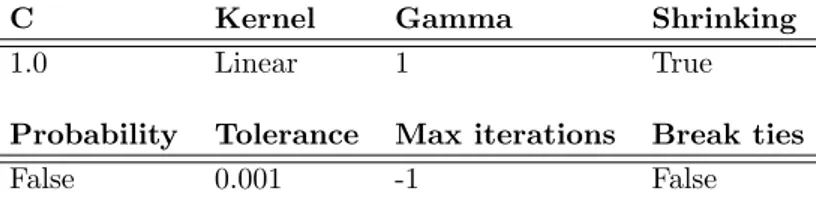
provided by the function was used, with an exception to the kernel function that was changed from an RBF kernel to linear kernel and to the gamma setting that was set to 1. The hyperparameters used for the SVM classifier can be seen in table 3.
C Kernel Gamma Shrinking
1.0 Linear 1 True
Probability Tolerance Max iterations Break ties
False 0.001 -1 False
Table 3: Hyperparameters for SVM classifier. In-depth explanations of the parameters can be found in the scikit-learn documentation6.
6.4..3 Logistic regression
Just as the SVM classifier, the LR algorithm was simple compared to the ANN. The scikit-learn library was used to implement this algorithm as well, but this time all of the default parameters initially set by the library was used. The relevant default parameters used for the LR classifier can be seen in table 4.
Penalty Dual Tolerance C
l2 False 0.0001 1
Fit intercept Solver Max iterations Multi class
True lbfgs 100 auto
Table 4: Hyperparameters for LR classifier models. In-depth explanation of the parameters can be found in the scikit-learn documentation7.
7.
Results
The results of each step in this study will be presented in the following subsections. This section have the same structure as section 6., which means that the results will be presented in the same order as they were obtained.
7.1.
GIF method evaluation
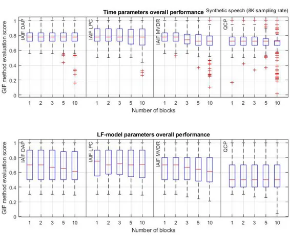
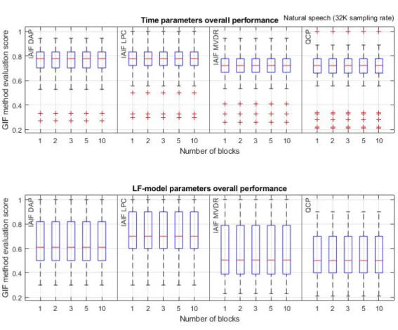
The evaluation of GIF methods showed that, for all GIF methods evaluated, the fraction of time domain parameters predicted within the accepted threshold (±20%) were higher than the fraction of LF-model domain parameters within the accepted threshold. This observation was consistent over both repositories (I and IV) and for the average score over both repositories. Figure 3 and 4 shows the distribution of the individual sample scores for each GIF method in the evaluation, as well as how the scores differed depending on the numbers of blocks used to divide the sub-samples in. A comparison of figure 3 and 4 shows that the GIF methods were less accurate on the samples stemming from repository IV (natural speech) than on the samples stemming from repository I (synthetic speech).
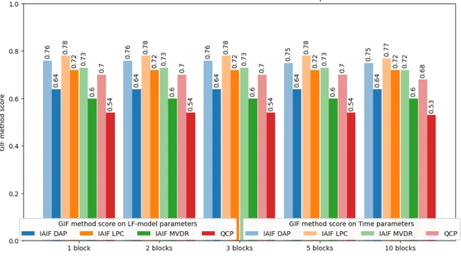
By looking at the different GIF method groupings in the two box plots (figure 3 and 4) we can see that the method accuracy seem to differ. Accuracy observed from the two figures seems to be, from highest to lowest: IAIF LPC, IAIF DAP, IAIF MVDR and lastly QCP. This observation is also consistent over both repositories as well as both parameter types. The accuracy order is uniform with the values shown in figure 5, which illustrates the average scores for both parameter types between the two repositories. The observation that LF-model parameters were less accurate that time domain parameters is also supported by the illustration in figure 5, since for every color pair (light and dark), the darker bar is lower than the lighter one in the pair. The dark bars represent the average GIF method score on the LF-model domain parameters, and the lighter bars on the time domain parameters.
7.2.
Machine learning models evaluation
All of the ML model evaluation values have been summarized in two tables, were each table show the values of the models split into time domain parameters and LF-model domain parameters. The cells of each value have been colored with a gradient from red to green depending on how good the value is in order to give the reader a quick overview of how good the value is. The evaluation scores for the models that used LF-model domain parameters can be seen in table 5, and the scores for the models that used time domain parameters can be seen in table 6.
Figure 3: A grouped box plots that illustrates the distribution of sample scores extracted from repository I (synthetic speech) for each of the GIF methods and parameter types. Each GIF method group also show how the distribution differed depending on the numbers of block-samples in each sample.
Figure 4: A grouped box plots that illustrates the distribution of sample scores extracted from repository IV (natural speech) for each of the GIF methods and parameter types. Each GIF method group also show how the distribution differed depending on the numbers of block-samples in each sample.
Figure 5: A grouped bar chart that displays the mean GIF method score of GIF done on repository I and IV. The lighter bars represent the mean scores when evaluated using time domain parameters, and the darker bars when using LF-model domain parameters. The bars are grouped into the numbers of block-samples that each sample were represented by.
7.2..1 Neural network
The GIF method used in a dataset did not seem to affect the performance of the model as much as initially thought. The ANN models performed remarkably well across all methods, and it seems that the number of block-samples used was a more of determining factor than the GIF method that was used to estimate the GFW. The models had worst performance when the numbers of blocks where 1, which also means that the size of the input vectors were the smallest (10 for LF-model domain parameters, and 18 for time domain parameters). Some models that used the LF-model parameters were noticeably affected by the number of block-samples, this can be seen by looking the performance of ANN models that used the IAIF DAP GIF method in table 5. These models got gradually better performance when the numbers of blocks used were increased. This pattern is not as consistent across the other GIF method groups (IAIF LPC, IAIF MVDR and QCP). Overall, the models that used the LF-model domain parameters performed worse than the models that used the time domain parameters, most noticeably when lower numbers of block-samples were used. By looking at ANN group in table 6, we can see that when using the time domain parameters and 2, 3, 5 or 10 blocks almost all models managed to classify everything correct, whereas in table 5 not as many perfect scores were reached. The ANN group in table 5 also shows that a higher number of blocks not necessarily gives a higher score, since the perfect scores were scattered across the different numbers of blocks. For example, the models that used QCP in combination with 2 blocks achieved an average of 1.0, where other models that used the same GIF method but higher number of blocks (3, 5 and 10) received a lower score. However, it is important to notice that the score differences are marginal and to remember that the training of ANN models is non-deterministic.
Evaluation on models using LF-model domain parameters ML model GIF
method
Macro average precision
1 block 2 blocks 3 blocks 5 blocks 10 blocks
ANN IAIF DAP 0.86 0.92 0.96 0.97 1.0 IAIF LPC 0.93 0.98 0.98 0.98 0.99 IAIF MVDR 0.81 1.0 0.97 1.0 1.0 QCP 0.97 1.0 0.99 0.98 0.99 SVM IAIF DAP 0.77 0.93 0.93 0.98 1.0 IAIF LPC 0.68 1.0 1.0 0.99 1.0 IAIF MVDR 0.61 1.0 1.0 1.0 1.0 QCP 0.88 0.95 0.94 0.95 0.97 LR IAIF DAP 0.74 0.84 0.85 0.86 0.90 IAIF LPC 0.64 0.83 0.87 0.9 0.92 IAIF MVDR 0.61 0.77 0.78 0.83 0.87 QCP 0.86 0.90 0.91 0.92 0.92
Table 5: Model evaluation scores when using LF-model domain parameters.
Evaluation on models using time domain parameters ML model GIF
method
Macro average precision
1 block 2 blocks 3 blocks 5 blocks 10 blocks
ANN IAIF DAP 0.97 1.0 0.99 1.0 1.0 IAIF LPC 0.91 1.0 1.0 1.0 1.0 IAIF MVDR 0.81 1.0 1.0 1.0 1.0 QCP 0.88 1.0 1.0 1.0 1.0 SVM IAIF DAP 0.94 1.0 1.0 1.0 1.0 IAIF LPC 0.82 1.0 1.0 1.0 1.0 IAIF MVDR 0.68 1.0 1.0 1.0 1.0 QCP 0.85 1.0 1.0 1.0 1.0 LR IAIF DAP 0.92 1.0 1.0 1.0 1.0 IAIF LPC 0.84 1.0 1.0 1.0 1.0 IAIF MVDR 0.68 1.0 1.0 1.0 1.0 QCP 0.84 0.96 0.96 0.96 0.96
7.2..2 Support vector machine
The SVM models showed a similar pattern as the ANN models, where the time domain parameters gave much better performance than the LF-model domain parameters. Tables 5 and 6 shows that the SVM models also had worst performance when using 1 block-sample. The models that used the time domain parameters consistently achieved a perfect score when using 2, 3, 5 or 10 blocks, which can be seen in table 6. The performance of the models that used the LF-model parameters are much more scattered than the models that used the time domain parameters. It also seems that the QCP group had worse overall performance than the IAIF LPC and the IAIF MVDR group, with an exception to when only 1 block-sample was used, in which the QCP group had much better performance. When looking at the 1 block-sample scores in tables 5 and 6, we can see that IAIF MVDR followed by IAIF LPC performed worst in both parameter type domains and that QCP performed comparatively well. This performance order is not consistent with the performance order that was displayed in figure 5, where QCP had the worst score in both parameter type domains, regardless of the number of block-samples.
7.2..3 Logistic regression
Just like the other ML models, the LR models had worse performance on the LF-model domain parameters, which can be seen in tables 5 and 6. The performance of the models that worked with the LF-model domain parameters seemed to have a correlation to the number of blocks used, where higher is better. This is shown for all GIF methods in the LR group of table 5, where the performance is almost always increasing when a higher number of block-samples are used. For the models that used the time domain parameters the case seems to be the opposite. By observing the performance on the 2, 3, 5 and 10 block-sample datasets in the LR group of table 6 we can see that the performances are equal. The QCP group is the most interesting group to look at since all mentioned block-sample numbers got a macro average precision of 0.96. This suggests that the performance already peaked at 2 block-sample datasets for LR models that used time domain parameters.
The LR models also had a significantly lower performance on the 1 block-samples for both param-eter types. The performance order seems to be almost uniform across the two paramparam-eter types, as well as with the 1 block performance order of the SVM models. The recurring pattern is that IAIF MVDR performs worst with 1 block-sample, followed by IAIF LPC. Overall, the LR models performed comparatively bad when put up against the other ML algorithms that used the same datasets.
7.3.
Combining the results
By combining the GIF method evaluation scores with the performances of the different ML models, potential correlations are easier to spot. Each of the evaluation scores in the previous sections were combined with the belonging GIF method evaluations scores. The goal of this is to find out if the score order and the precision order ever were the same. All of the combined graphs can be found in appendix A. By looking at the combined figures in appendix A (figure A.1, A.2, A.3, A.4, A.5 and A.6) we can see that this was almost never the case. The models that used QCP datasets seemed to be the main culprits for breaking the order by having low GIF method scores and relatively high ML model performance scores. However, some patterns can be spotted in some of the figures, for example in figure A.3 where we can see bit of correlation between GIF evaluation score and model performance in the sense that models that used QCP datasets generally performed worse than models that used IAIF LPC based and IAIF MVDR based datasets. Another figure with some patterns were figure A.5. This illustration shows a little bit of correlation between model performance and GIF method evaluation score in the 3, 5 and 10 block groups. The precision and score order is uniform for IAIF LPC, IAIF DAP and IAIF MVDR in these block groups, while
QCP breaks the pattern by performing very good with regards to GIF evaluation scores.
The ANN and SVM models showed the least correlation between GIF method evaluation score and model performance, since they both seemed to be able to get near perfect scores regardless of which parameter type or GIF method that was used to create the datasets. The models that showed the most correlation were the LR models. Particularly the models that used the LF-model domain parameters (figure A.5) where the GIF method score and the model score order were consistent for (from best to worst) IAIF LPC, IAIF DAP and IAIF MVDR in the 3, 5 and 10 block groups.
8.
Discussion
The results from the ML experiments showed that generally, a higher number of block-samples are preferred when striving for high precision. The reason for this could be that the individual characteristics of each class (synthetic and real) are better represented when more block-samples are present, or because of the increased number of features in the input vectors. It is also possible that the reason is a combination of both. The same reasoning should be applied when looking at the higher performance of the models that used the time domain parameters versus those that used the LF-model domain parameters. The higher performance on the time domain parameters could be because they were more accurate, or because they were 1.8 times as many (18 time parameters vs. 10 LF-model parameters in each block-sample), or yet again, a combination of both options. The results presented in tables 5 and 6 suggests that it is a combination of both. A block-wise comparison shows that the time domain parameter datasets performed better regardless of the number of blocks (with a few exceptions) and that the LF-model domain parameter datasets’ performance increased when more block-samples were used, which also meant that the input input vectors were bigger.
With the assumption that the metric used for GIF method evaluation gives a good representation of how accurate the estimated GFWs are, the results suggest that no obvious correlation between GFW accuracy and SSD algorithm performance exist. Figures A.1, A.2, A.3, A.4, A.5 and A.6 supports this claim since they do not show any patterns that would suggest otherwise. If both the lighter and the darker bars would have shown similar patterns, the conclusion would be the opposite.
It is worth considering that even though the GIF methods got different evaluation scores, there is a high chance that some of them had more or less equal accuracy on some parameters that could play a key role in the ML models’ ability to correctly classify the samples. For example, the authors of [4] confirmed the usefulness of certain parameters in a parametrized GFWs. If the GIF methods evaluated in this study were accurately estimating GFWs that, when parametrized, gave accurate values on useful parameters, and inaccurate values on less useful parameters, it could mean that the evaluation score inaccurately depicts the performance of the GIF methods. This could in turn affect perceived correlation between GFW accuracy and SSD performance, or the lack of it. It is also possible that ML models learned to use the accurate values, and ignore less accurate values when classifying the samples. This means that the accuracy of each parameter as well as the importance of the parameter in the ML models should be investigated further to confirm or falsify the results of this thesis.
8.1.
Limitations
Due to time constraints associated with this thesis, a lot of unforeseen limitations appeared along the way. Some of these limitations might have been easily solved by an expert in the field, but since I am no expert in this field, some corners had to be cut and assumptions had to be made. To address the limitations in chronological order, the large scale GIF needs to be discussed first. As mentioned earlier, Aalto Aparat was not created for quickly performing GIF on large set of samples. The features as well as the interface of the tool suggests that each sample should be treated with care and manually inspected by a trained eye to be able to get the best results by iteratively fine-tuning the hyperparameters. Time consuming manual labor is not desirable when time is of the essence, as it was during this thesis. Automatic extraction was a must, so automated large scale GIF and parametrization at the cost of varied sample quality was the best option. It is hard to identify the magnitude of the varied sample quality without performing the manual labor for each of the samples and then comparing the results with the automated ones. However, it is clear from figure 3 and 4 that the samples in repository IV (natural speech) were noticeably affected by the automation process since the accuracy is generally lower than for the samples in
repository I.
Another limitation lies in the nature of the two used OPENGLOT repositories. Repository I had a lot more samples than repository IV, and the sampling rate was 8KHz and 44.1KHz respectively, which heavily influences the sound quality of the samples. It is possible that this sampling rate difference was somehow revealed in the extracted parameters and that it was the reason for the perfect scores that some ML models got. This needs to be investigated further by performing the experiments with datasets that have the same sampling rate to see if the results are consistent with the results in this study.
Next up we have the GIF evaluation method. In [4], the authors used a similar method, but on less GIF techniques and fewer extracted parameters, which made it possible to find characteristics of the used techniques and individually evaluate the samples as well as the parameters. However, in this thesis there were too many samples, and too many GIF methods for individual inspection to be a viable option. The evaluation method created in this thesis aims to give an abstract view of the overall performance of the methods. This abstraction may have caused important details to be obscured and thus not be considered in the final evaluation. However, the results from the evaluation in figure 3, 4 and 5 suggests that the abstract evaluation was successful, as long as we assume that by varying GIF method and settings, we should expect to get varying evaluation scores.