Oxidation of Graphite and Metallurgical Coke: A Numerical Study with an Experimental Approach

IN

DEGREE PROJECT MATERIALS DESIGN AND ENGINEERING,

SECOND CYCLE, 30 CREDITS ,

STOCKHOLM SWEDEN 2016

Oxidation of Graphite and

Metallurgical Coke

A Numerical Study with an Experimental

Approach

YOUSEF AHMAD

KTH ROYAL INSTITUTE OF TECHNOLOGY

Abstract

At the royal institute of technology (KTH) in the department of applied process metallurgy, a novel modelling approach has been developed which allows a dynamic coupling between the commercial thermodynamic software Thermo-Calc and the commercial computational fluid dynamic (CFD) software Ansys Fluent, only referred to as Fluent in the study. The dynamic coupling approach is used to provide numerical CFD-models with thermodynamic data for the thermo-physical properties and for the fluid-fluid chemical reactions occurring in metallurgical processes. The main assumption for the dynamic coupling approach is the existence of local equilibrium in each computational cell. By assuming local equilibrium in each computational cell it is possible to use thermodynamic data from thermodynamic databases instead of kinetic data to numerically simulate chemical reactions. The dynamic coupling approach has been used by previous studies to numerically simulate chemical reactions in metallurgical processes with good results. In order to validate the dynamic coupling approach further, experimental data is required regarding surface reactions. In this study, a graphite and metallurgical coke oxidation experimental setup was suggested in order to provide the needed experimental data. With the experimental data, the ability of the dynamic couplings approach to numerically predict the outcome of surface reactions can be tested.

By reviewing the literature, the main experimental apparatus suggested for the oxidation experiments was a thermo-gravimetric analyzer (TGA). The TGA can provide experimental data regarding the reaction rate, kinetic parameters and mass loss as a function of both temperature and time. An experimental setup and procedure were also suggested.

In order to test the ability of Fluent to numerically predict the outcome of surface reactions, without any implementation of thermodynamic data from Thermo-Calc, a benchmarking has been conducted. Fluent is benchmarked against graphite oxidation experiments conducted by Kim and No from the Korean advanced institute of science and technology (KAIST). The experimental graphite oxidation rates were compared with the numerically calculated graphite oxidation rates obtained from Fluent. A good match between the experimental graphite oxidation rates and the numerically calculated graphite oxidation rates were obtained. A parameter study was also conducted in order to study the effect of mass diffusion, gas flow rate and the kinetic parameters on the numerically calculated graphite oxidation rate. The results of the parameter study were partially supported by previous graphite oxidation studies. Thus, Fluent proved to be a sufficient numerical tool for numerically predicting the outcome of surface reactions regarding graphite oxidation at zero burn-off degree.

Content

1 Introduction ... 1

1.1 Metallurgical Coke ... 4

1.1.1 Manufacturing process ... 4

1.1.2 Blast furnace process and oxidation of metallurgical coke ... 5

1.2 Graphite ... 8

1.2.1 Manufacturing process ... 8

1.2.2 Graphite oxidation ... 10

1.2.3 The effect of the temperature on the graphite oxidation rate ... 10

1.2.4 The effect of the gas flow rate on the graphite oxidation rate ... 13

1.2.5 The off-gas composition ... 13

1.3 Mathematical and CFD-modeling of graphite oxidation ... 15

1.4 Previous studies regarding the experimental setup for oxidation experiments ... 17

1.4.1 Thermogravimetric analysis ... 18

1.4.2 The graphite oxidation experiment by Kim and No [31] ... 20

2 Method ... 22

2.1 Suggesting experimental apparatus and setup ... 22

2.2 Numerical setup ... 23

2.2.1 Computational domain and mesh ... 23

2.2.2 Surface reaction model and governing equations ... 24

2.2.3 Graphite oxidation model and kinetic parameters ... 30

2.2.4 Main assumptions and boundary conditions ... 33

3 Results ... 34

3.1 Suggested experimental setup ... 34

3.1.1 Experimental equipment’s ... 35

3.1.2 Sample material ... 37

3.1.3 Experimental gases and gas flow rates ... 37

3.1.4 Experimental procedure ... 37

3.2 Numerical study ... 40

3.2.1 Calculated numerical parameters ... 40

3.2.2 Graphite oxidation simulation ... 41

4 Discussion ... 44

4.1 Experimental apparatus and setup ... 44

4.1.2 Off-gas measurements ... 45

4.1.3 Sample attachment ... 46

4.2 Numerical simulations ... 46

4.2.1 The graphite oxidation rate dependence on the oxygen concentration and surface temperature ... 46

4.2.2 The graphite oxidation rate dependence on the mass diffusion and the gas flow rate ... 47

4.2.3 The graphite oxidation rate dependence on the kinetic parameters ... 48

5 Conclusion ... 50

6 Acknowledgement ... 50

1

1 Introduction

At the present day, the use of computers to run numerical simulations of various complex science and engineering problems has increased due to the development of cheaper and more powerful computers. The use of numerical simulations has been known to decrease the amount of trial and error experiments traditionally required in order to obtain partial information of physical phenomenon in a science or engineering problem. Numerical simulations may also be used to provide information regarding physical situations which would not be possible to set up experimentally due to huge expenses or ethical reasons. By making the right assumptions and simplifications, numerical simulations are used by scientist and engineers as tools for solving problems concerning a wide range of fields [1].

At the KTH in Stockholm, Sweden, in the division of applied process metallurgy, numerical simulations are used to numerically predict outcomes regarding process phenomena, primarily regarding steel making. [2]

Recently, a novel modeling approach between CFD and thermodynamics has been developed at KTH. The novel modeling approach is a dynamic coupling between a commercial CFD-software, Fluent, and a commercial thermodynamic software, Thermo-Calc.

In Thermo-Calc it is possible to calculate phase equilibria and perform other thermodynamic related calculations for a variety of metallurgical systems by using data from thermodynamic databases. The thermodynamic databases in Thermo-Calc are validated both experimentally and theoretically by following the Calphad method. Thermo-Calc databases thus provides established thermochemical and thermo-physical data to the user.

Fluent is a powerful commercial CFD-software that enables broad modeling capabilities regarding fluid flow, heat transfer, turbulence and multi-phase simulations. Thus, Fluent has the computational capabilities to simulate vast amount of technological applications ranging from combustion and chemical reactors to aeronautics and blood flow. [3]

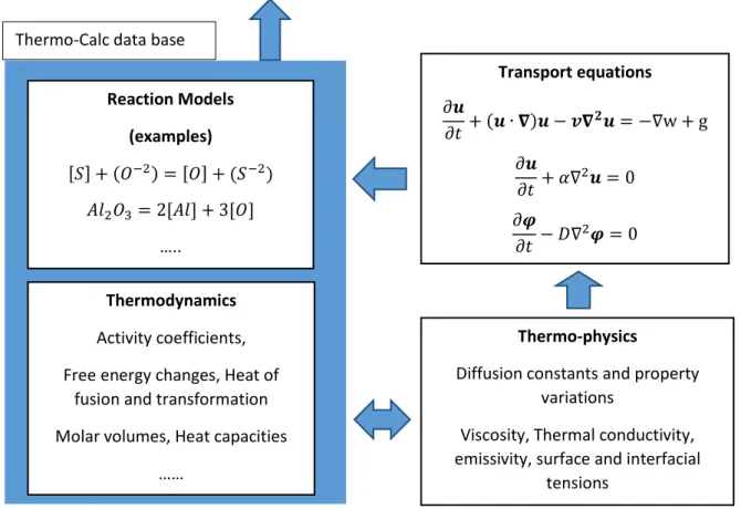
The main assumption for the dynamic coupling approach is that in each computational cell a local equilibrium is established during the course of each time step. In other words, by making the computational cells relatively small it is possible to assume that a local equilibrium is reached in each computational cell and thereby it is justified to use thermodynamic data instead of kinetic to numerically simulate chemical reactions [4]. By combining transport equations of the momentum transport, heat transport, mass transport with the thermodynamic databases provided by Thermo-Calc it is be possible to numerically simulate a reacting flow in a multiphase simulation. The reactive flow can be numerically simulated without the necessity of having experimental data for the kinetic parameters such as reaction frequency factor, rate constants, reaction order and other important chemical kinetic parameters which traditionally are case dependent and are crucial in order to simulate transient chemical reactions. The relationship between the transport equations and thermodynamic data, suggested by Jonsson et al. [5] and Ersson et al. [4] can be seen in Figure 1.

2

Figure 1: The schematics of the numerical approach of the idea of coupling between CFD and thermodynamics. Taken from references [4] [5].

The dynamic coupling approach has provided good results when applied to a numerical simulation of a top-blown converter in steel making process. The dynamic coupling approach has only been used to simulate fluid-fluid chemical interactions by using the volume of fluid model to numerically simulate the gas, slag and steel phase. [4]

The numerical algorithm for the dynamic coupling approach can be seen in Figure 2.

Transport equations 𝜕𝒖 𝜕𝑡+ (𝒖 ∙ 𝛁)𝒖 − 𝒗𝛁𝟐𝒖 = −∇w + g 𝜕𝒖 𝜕𝑡 + 𝛼∇2𝒖 = 0 𝜕𝝋 𝜕𝑡 − 𝐷∇2𝝋 = 0 …. Thermo-physics

Diffusion constants and property variations

Viscosity, Thermal conductivity, emissivity, surface and interfacial

tensions Thermo-Calc data base

Thermodynamics

Activity coefficients, Free energy changes, Heat of

fusion and transformation Molar volumes, Heat capacities

…… Reaction Models (examples) [𝑆] + (𝑂−2_{) = [𝑂] + (𝑆}−2₎ 𝐴𝑙₂𝑂₃= 2[𝐴𝑙] + 3[𝑂] …..

3

The explanation of each step in the algorithm is taken from Ersson et al. [4], see below: a) The model is initialized with initial values.

b) The transport equations are numerically solved.

c) If the existing phases in each computational cell is larger than a minimum pre-defined value Thermo-Calc is called upon to calculate equilibrium.

d) The newly calculated temperature and species distribution are set. The mass transfer between the phases is stored and used in the subsequent time step.

e) A check is done in order to control the convergence of the calculations.

f) If convergence has been reached the program terminates. Otherwise it jumps back to step b) using the newly obtained variables.

In steel making processes, there are several external factors which can interfere with measurements and thereby provide experimental artifacts. In other words, the output data in steel making has a lot of uncertainties and uncontrollable factors which is not easily isolated and identified. This suggest that more controlled experimental data is needed in order to benchmark the dynamic coupling approach.

The first objective of this degree project was to find the most suitable experimental apparatus and setup for graphite-and metallurgical coke oxidation. The experimental result could then be used for benchmarking the dynamic coupling approach against primarily surface reactions, since the dynamic coupling approach has never been benchmarked against surface reactions before.

The second objective was to test the commercial CFD-software Fluent to numerically predict the outcome of surface reactions relating to graphite oxidation. This was conducted by benchmarking Fluent against a previous graphite oxidation study.

a) b) c) d) e) f) Init

Solve transport equations (CFD)

Calculate local equilibrium (Thermo-Calc)

Update CFD-program

t=tN?

end

4

1.1 Metallurgical Coke

1.1.1 Manufacturing process

Metallurgical coke is the common name for black coal that goes through a pyrolysis process, a heat treatment in a non-oxygen environment. In the pyrolysis, volatile compounds such as hydrocarbons and moisture is evaporated from the black coal. The product of the pyrolysis is a carbon rich and porous material. [6]

There are several important factors when producing metallurgical coke for the blast furnace process. In the blast furnace process the metallurgical coke is used as fuel, reduction agent and structural material. The production of metallurgical coke takes place in a cooking oven located at a cooking plant, see Figure 3.

Figure 3: A cooking oven at the company DPL in India [7].

Before the black coal arrives at the cooking oven, there are several pre-treatments of the black coal which need to be conducted to ensure that the metallurgical coke obtains high quality. The general manufacturing steps of metallurgical coke can be seen in Figure 4.

Figure 4: The production steps in the manufacturing process of metallurgical coke for usage in the blast furnace process [8]. First, various types and grades of black coals are mixed together in a mixing bin. Then the mixed black coal is crushed into powder and screened so that the right particle sizes are obtained. The coal powder is then pre-heated to approximately 200°C in order to prepare the coal powder for the pyrolysis in the coke oven. The pre-heated coal powder is then delivered to the coke oven where the coal powder is further heat treated at temperatures ranging from 1000-1400°C in a low oxygen environment for approximately 16-24 hours [6]. During the cooking process, volatile hydrocarbons

5

and water are evaporated from the coal powder while the carbon particles begins to agglomerate and form bigger pieces. The off-gases from the coke oven are collected and directed for further chemical treatment so that the byproducts such as benzene and tar are extracted and stored. The off-gas may also be stored and used as fuel for the cooking plant. When the cooking process is completed, the produced metallurgical coke is water quenched and cooled before it is transported and used in the blast furnace process.

The finished metallurgical coke consist mainly of carbon but there is some traces of Sulphur and phosphorus. The metallurgical coke may also contain traces of aluminum- and silicon oxide. [6]

1.1.2 Blast furnace process and oxidation of metallurgical coke

There are two main process routes in steel making. There are the integrated steel making route and electrical arc steel making route, see Figure 5.

Figure 5: The schematics for the production of steel by scrap or iron ores [9].

In the integrated steel production route, the blast furnace process main objective is to produce liquid pig iron by the reduction of iron ores. A blast furnace can produce approximately 1200 tons of liquid pig iron per day and use approximately 85-90% of all the heat that is produced in the process. [6] The blast furnace process is a continuous process where the input materials such as iron ore, slag formers and metallurgical coke are charged at the top of the blast furnace while the end products, liquid iron and slag, are tapped from tap holes in the bottom of the furnace.

The input material passes through different temperature zones inside the blast furnace and after several chemical reactions turns into the end products. The temperature zones are zones with different temperatures and therefore have chemical reactions with different kinetic conditions. The temperature zones in the blast furnace, from the top to the bottom of the furnace, are listed below.

6 1) The pre-heating zone

2) The thermal reserve zone

3) Direct reduction and melting zone.

The schematics of a blast furnace can be seen in Figure 6.

Figure 6: The schematics of a blast furnace process [10].

In the pre-heating zone the temperature increases from room temperature to approximately 800°C. In the pre-heating zone, the raw material is heated by circulating gases inside the blast furnace which originates from the pre-heated oxygen enriched air (blast) injected into the blast furnace from the tuyeres and from the off-gases form the chemical reaction occurring in the lower part of the furnace. The pre-heating contributes to the removal of volatile compounds which can reside in the raw material. The first indirect reduction is when the hematite, 𝐹𝑒2𝑂3, is reduced to magnetite, 𝐹𝑒3𝑂4. This occurs when the hematite reacts with the carbon monoxide in the circulation gas, see reaction R1.

The circulation gas mainly consist of carbon monoxide, carbon dioxide and nitrogen gas. The second indirect reduction occurs when the magnetite is reduced to iron oxide, 𝐹𝑒𝑂, see reaction R2.

3 𝐹𝑒₂𝑂₃+ 𝐶𝑂 = 2 𝐹𝑒₃𝑂₄+ 𝐶𝑂₂ (R1)

3 𝐹𝑒2𝑂3+ 𝐶𝑂 = 2 𝐹𝑒3𝑂4+ 𝐶𝑂2 (R2)

In the thermal reserve zone the charged input material obtains the same temperature as the circulating gas. The temperature in this zone is in between 800-1000°C. In the thermal reserve zone most of the indirect reduction of iron occurs. The indirect reduction reaction proceeds according to reaction R3.

7

𝐹𝑒𝑂 + 𝐶𝑂 = 𝐹𝑒 + 𝐶𝑂₂ (R3)

The final zone is the melting and direct reduction zone. In the melting and direct reduction zone any unreduced iron oxide is reduced to iron by direct reduction, see reaction R4. In the melting and direct reduction zone the temperature is between 1400-2000°C. So melting and mixing between iron and slag formers occurs. As mentioned earlier, blast is injected through tuyeres located at the furnace walls near the bottom. The oxygen in the blast is used to combust the metallurgical coke to provide the energy required for the furnace to maintain its operational temperature, see reaction R5 and reaction R6 [11]. The metallurgical coke is also used as main reduction agent for reducing oxides, see reactions R7-R10. 𝐹𝑒𝑂 + 𝐶𝑂 = 𝐹𝑒 + 𝐶𝑂 (R4) 𝐶 + 𝑂2= 𝐶𝑂2 (R5) 𝐶 +1 2𝑂2= 𝐶𝑂 (R6)

Other direct reduction reactions which occur in the melting and direct reduction zone is seen below

𝐶𝑎𝐶𝑂₃+ 𝐶 = 𝐶𝑎𝑂 + 𝐶𝑂₂ (R7) 𝑀𝑛𝑂 + 𝐶 = 𝑀𝑛 + 𝐶𝑂 (R8) 𝑃₂𝑂₅+ 5 𝐶 = 2𝑃 + 5 𝐶𝑂 (R9) 𝑆𝑖𝑂₂+ 2 𝐶 = 2𝑆𝑖 + 2𝐶𝑂 (R10)

The carbon monoxide gas is formed from reactions together with the blast and then transports the heat produced from the reactions to the top zones of the blast furnace. As mentioned earlier, the carbon monoxide is used for indirect reduction of reducing hematite, magnetite and iron oxide. The formed carbon dioxide is used to produce carbon monoxide by the Boudouards reaction which is the largest endothermic reaction within the blast furnace process, see R11.

8

1.2 Graphite

Graphite is a porous carbon based crystalline material with a hexagonal crystal structure (HCP), the carbon basal planes of the HCP-structure are displayed in Figure 7.

Figure 7: The basal planes of carbon atoms in graphite [12].

Graphite has a wide range of technical applications due to its high electrical conductivity, chemical inertness, and good mechanical properties in high temperatures etc. Graphite can be found in engineering application at, for example, the nuclear energy industry, steel industry and electronic industry. [13]

1.2.1 Manufacturing process

It is possible to find natural deposits graphite at some places in the world such as China and South America [14]. In this study focus is on synthetic graphite, which includes both so called carbon graphite and electro graphite. Therefore, this study do not involve any more information regarding so called natural graphite.

Synthetic graphite is produced mainly from special types of carbon sources which are made into a specific powder. The carbon sources mainly originates from petroleum coke, pitch coke and carbon black. The carbon sources may also originate from secondary graphite, re-used graphite. [15] [16] During the powder preparation, see Figure 8, the carbon sources are first separated and stored in silos. Then the carbon sources are mixed, crushed and pulverized in order to obtain a fine powder, also known as carbon powder. The carbon powder is then screened in order to obtain the right particles sizes and particle size distribution. The particles which fail to pass the required demands on particles size is returned back to the crushing and pulverizing step. When the carbon powder has obtained the right particle sizes and particle size distribution, the carbon powder is mixed together with a binder. The binder usually consist of coal tar pitch or synthetic resins. The binder provides some enhancement to the mechanical properties of the green body. [15] [16]

9

Figure 8: The powder preparation in the manufacturing process of graphite. [17]

When the carbon powder has blended together with the binder the carbon powder is sent to a shape forming process where the green body is formed. The shape forming processes are mainly extrusion, isostatic pressure or die molding. The shape forming process is chosen in regard to the required properties and shape of final product. The main outcome of the shape forming process is a compressed and formed green body. [15] [16]

After the shape forming process, the green body is baked (heat treated) in a furnace by pyrolysis at approximately 1000-1200°C for one to two months to remove volatile compounds, such as binders and hydrocarbons, and initiate the formation of elementary carbon which can bind the carbon powder particles together. Since the newly bonded carbon particles cannot replace the volume of the evaporated volatile hydrocarbons and binder pores are formed in the heat treated material. After the baking process the material is amorphous, brittle and hard. The material is known as carbon graphite. [18]

The final step of the graphite manufacturing process is the graphitization, which is a heat treatment at approximately 3000°C conducted for one to three weeks. At the graphitization, the last impurities such as residual binders, oxides and sulfur etc vaporizes and leaves the graphite thus increasing the purity of the graphite. At these high temperatures the carbon atoms starts to realign themselves from the previously amorphous structure into a HCP crystal structure. [16] [18]

There are further refining treatments to produce synthetic graphite with even lower amounts of impurities and with less porosity. The further refining treatments are essential in order to produce so called special graphite which are used in applications where the demands on the purity and mechanical properties are high. In the nuclear energy industry the demands for high quality special graphite is crucial in order to provide the structural material to withstand the corrosive atmosphere

10

inside of a high temperature reactor. The impurities in graphite consist mainly if metallic elements such as titanium, vanadium and iron etc. The metallic impurities are referred to as ash.

1.2.2 Graphite oxidation

Graphite is generally considered an inert material at standard temperatures and pressure. When graphite is exposed to higher temperatures and strong oxidizing atmospheres graphite will start to decompose by the oxidation. When graphite reacts with oxygen, mainly two oxidation reactions occurs, see reactions R12 and R13.

𝐶(𝑔𝑟) +1

2𝑂2= 𝐶𝑂 (R12)

𝐶(𝑔𝑟) + 𝑂₂ = 𝐶𝑂₂ (R13)

There are other compounds which may oxidize graphite besides oxygen that can be used to oxidize the carbon in the graphite such as water vapor and carbon dioxide. From here on oxygen is considered the main and only oxidizer.

A simplified version of the oxidation mechanism steps I seen below, from A-D.

A) The oxygen gas molecules diffuses from the bulk flow of the atmosphere to the graphite surface.

B) The oxygen gas molecules comes in contact with an active site, a favorable site on the graphite basal planes where a reaction can occur and these sites are normally found on the edges of the basal planes [19], or it continues to diffuse further into the graphite porous network and finds another active site in the interior parts.

C) The oxygen gas molecule disassociate and adsorbs onto the active site where it reacts with a reactive carbon and forms gas products or a surface oxide complex [20]. This surface oxide complex can also turn into a gaseous product when reacting with another disassociated oxygen atom, in other words the surface complex acts an intermediate in the production of the gaseous products.

D) The gaseous product desorbs from the active site and migrates out of from the porous network and diffuses out of the graphite to the outer atmosphere [21].

1.2.3 The effect of the temperature on the graphite oxidation rate

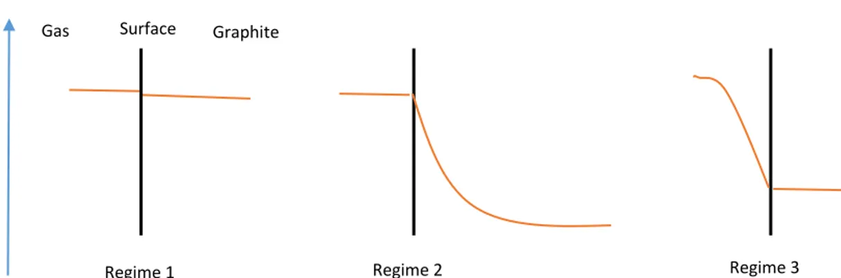
The graphite oxidation rate is, to a very high degree, temperature dependent. The temperature dependence of the graphite oxidation rate is manifested into three different temperature zones or regimes where the graphite oxidation rate has different rate-limiting steps [22]. The name of these temperature regimes can be seen below. The temperature regimes are listed from low temperature to high temperature.

1) The chemical regime

2) The in-pore diffusion regime 3) Boundary layer controlled regime

The schematics of the effect of the temperature regimes on the oxygen concentration adjacent to the graphite surface can be seen in Figure 9.

11

In the chemical regime, the graphite oxidation rate is relatively low due to relatively high activation energy for the oxidation reaction. As the name of the temperature regime implies, the graphite oxidation rate is limited by the chemical reaction between the oxygen and the reactive carbon in the graphite. The relatively low graphite oxidation rate allows the oxygen to diffuse deep into the graphite porous network before reacting at an active site. The result of the deeper diffusion is that the graphite oxidation becomes much more homogenously distributed within the graphite [22] [23]. An increase in porosity and pore size is seen in the chemical regime as a consequence of the homogenous oxidation. No major changes of the geometry is found in this regime since the graphite is oxidized and consumed mainly by pore formation in the interior part of the graphite. [24]

When the temperature reaches approximately 800-1050°C, see Table 1, the oxidation enters into the last temperature regime which is the boundary layer controlled regime. In the boundary layer controlled regime the reaction rate is very high and the graphite oxidation rate reaches saturation, small or no increase in graphite oxidation rate with higher temperature [23]. The oxidation reactions are limited to the graphite surface and therefore there is almost no oxygen diffusion into the porous network. In the boundary layer controlled regime the gas diffusion or the mass transport to the graphite surface is the rate-limiting step since the oxidation reactions are occurring very rapidly when the oxygen comes in contact with the graphite. [21]

When the temperature is between the interval of the chemical regime and the boundary layer controlled regime, the graphite oxidation enters in to the in-pore diffusion regime. The in-pore diffusion regime is a mixture between the chemical regime and the boundary layer controlled regime. In the in-pore diffusion regime the reaction rate is relatively higher than in the chemical rate regime [19], the reactions occur more frequently relative to the chemical rate regime. In the in-pore diffusion regime the rate-limiting step is a combination of both the chemical reaction and the mass diffusion. The oxidation reaction occurs closer to the graphite surface than in the chemical regime but the diffusion into the porous network are still occurring. The limitation of the diffusing depth makes it more difficult for the oxygen to oxidize the inner parts of the graphite. [21]

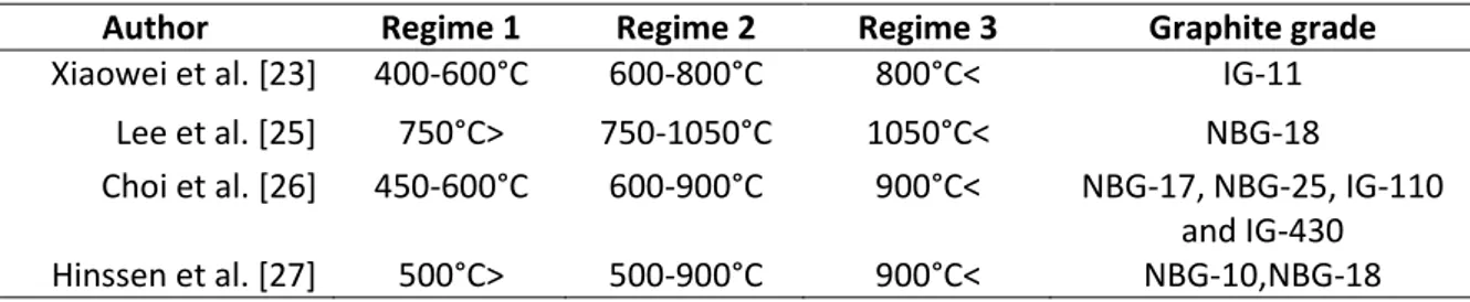
The temperature intervals for the temperature regimes for some common graphite grades can be seen in Table 1.

Oxygen concentration

Regime 1 Regime 2 Regime 3

Graphite Gas

Figure 9: Schematic plots of oxygen concentration inside and outside the graphite for the three temperature regimes.

Surface e

12

Table 1: The temperature intervals for the different oxidizing regimes in some common special graphite grades according to previous studies.

Author Regime 1 Regime 2 Regime 3 Graphite grade

Xiaowei et al. [23] 400-600°C 600-800°C 800°C< IG-11 Lee et al. [25] 750°C> 750-1050°C 1050°C< NBG-18

Choi et al. [26] 450-600°C 600-900°C 900°C< NBG-17, NBG-25, IG-110 and IG-430 Hinssen et al. [27] 500°C> 500-900°C 900°C< NBG-10,NBG-18

The temperature regime intervals and their transition temperatures depends on several manufacturing parameters such as graphite density, impurity concentration and microstructure [28]. There are some factors which can affect the oxidation rate independently of the temperature. These factors are listed below, from 1-5. [21] [22] [27]

1) The porosity 2) The ash content

3) The oxidizer concentration 4) The degree of graphitization 5) The burn-off degree

The graphite manufacturing process has an impact on the initial porosity. The porosity will affect how much oxygen that comes in contact with the active sites of the graphite. The total active site area (ASA) is decreased when the mean pore size is increased, less oxidation per volume occurs which results in decreased graphite oxidation rate. In the chemical regime the graphite oxidation rate is favored by relatively large pores since large pores allows more oxygen to diffuse into the porous network and increase the graphite oxidation rate by increasing the probability of an oxygen reacting with a carbon at an active site. At higher temperature, in the boundary layer controlled regime, large pores decrease the oxidation rate since the oxidation reaction mainly takes place at the graphite surface. At the graphite surface, larger pores will decrease the ASA and thereby decrease the graphite oxidation rate. A much denser graphite, smaller pore sizes and less porosity, will thus provide a greater ASA at the surface and that will increase the graphite oxidation rate. [19]

Another important factor is the ash content in the graphite. In graphite, elements such as Al, Ti, V, Fe Ni and Mg etc are considered impurities and are called ash [21]. The metallic elements in the ash are seen to have a catalytic effect on the graphite oxidation and thus decrease the activation energy for the graphite oxidation reaction and thereby weakens the oxidation resistance. The catalytic effect result in a higher graphite oxidation rates at lower temperatures. The catalytic effect of the ash on the graphite oxidation rate only last until approximately 750°C for some common graphite grades such as IG-110. [29] Above that temperature, the effect of the temperature on the graphite oxidation rate is greater than that of the impurities.

The oxidizer concentration within the carrier gas or in the atmosphere is also an important factor that affects the graphite oxidation rate. The oxidizer diffuses through the atmosphere or the carrier gas to the graphite surface. If there is not enough oxidizing elements within the atmosphere or the carrier gas the graphite oxidation rate will be low relative to an atmosphere or carrier gas rich in oxidizers. The diffusion properties, supply and availability of oxidizing elements thus are rate limiting factors. This is seen naturally in the boundary layer controlled regime where the diffusion of oxidizer is the rate-limiting step. So generally, the higher the concentration is of the oxidizers in the

13

atmosphere the higher is the oxidation rate. More oxidizers results in a higher probability that reactions could occur on the active sites. [21] [30] [31]

Another factor is the graphitization degree which is affected by the graphitization process during manufacturing. As mentioned earlier, the graphitization is a heat treatment process where a phase transformation occurs, the graphite change crystal structure from an amorphous structure into a crystalline. The graphitization degree is the ratio between the amounts of formed crystalline graphite relative to the initial amorphous graphite. The higher the graphitization degree the higher percentage of the graphite material consist of crystalline graphite. Previous studies states that the active sites, which are most likely to react with oxygen, are mostly located on the edges and ends of the basal planes of the HCP-structure [13] [19]. With a higher graphitization degree there are less active sites available in the graphite due to formation of bonds between the carbon atoms and thereby the graphite obtains a natural resistance towards oxidation which decreases the graphite oxidation rate relative to a graphite with low graphitization degree [32].

During oxidation, graphite is consumed or burned off over time due to the oxidation reaction. The burn-off degree is defined as the ratio between graphite which has been consumed over time and the initial graphite mass [21] [23] Previous studies have shown that the graphite oxidation rate is dependent on the burn-off degree since it has been seen that when graphite is oxidized closed porosity is opened and new pores are formed which increase the total ASA of the graphite [19] [21] [33]. The increase in graphite oxidation rate with burn-off degree is only observed at burn-off degrees lower than 40% [33]. After approximately 40% burn-off degree it is believed that the pores join each other and form macro pores. Macro pores decreases the total ASA and thereby decreases the overall graphite oxidation rate.

1.2.4 The effect of the gas flow rate on the graphite oxidation rate

The effect of the gas flow rate on the graphite oxidation rate has been investigated and studied by several previous studies. In a study conducted by Chi et al. [34] An investigation of the gas flow rate effect on graphite oxidation concerning the graphite grades NBG-18 and NBG-25 was conducted. The experiments were conducted in a vertical tube furnace (VTF) from ASTM with several flow rates within the interval of 1-10 L/min. It was concluded from their study that the effect of the gas flow arte on the graphite oxidation rate is temperature dependent and the gas flow rate generally increases the graphite oxidation rate when the temperature is higher than 700°C. [34]

The gas flow rate has been seen to have an impact on the thickness of the boundary layer which forms in the boundary layer controlled regime. A high flow rate will make the boundary layer thinner since the bulk flow will mechanically force the product gas away, thus the high flow rate of the inlet gas influences the transportation and removal of product gases away from the surface of the graphite. [35]

Another study was conducted by Takahashi et al. [30] in which the oxidation behavior of the graphite grade IG-110 was investigated. It was observed that the graphite oxidation rate increases with higher gas flow rate relative to the lower gas flow rate. The gas velocity also seemed to effect the rate at which carbon monoxide were formed in respect to temperature.

1.2.5 The off-gas composition

When graphite is oxidized by oxygen there are several chemical compounds which can form, carbon monoxide, carbon dioxide and surface oxide complexes. According to previous studies, both carbon monoxide and carbon dioxide are considered to be primary products and that the ratio between then mainly dependents on the temperature, burn-off degree and oxygen concentration in the

14

atmosphere or carrier gas [20]. According several previous studies, the off-gas composition is also affected by the gas pressure and the gas flow rate. [36] [37] [38]

At higher temperatures the main compound found in the off-gas is carbon monoxide [31] [30]. There are some indications that the Boudouard reactions is partially responsible for the graphite oxidation at high temperatures. [36]

Guldbransen et al. [37] conducted online off-gas analysis during a graphite oxidation experiments by using mass spectrometry to analyze the off-gas composition. It was concluded that study that at 1200°C, with a total pressure of 5-9 torr, the off-gas mainly consisted of carbon monoxide when injecting both commercial oxygen gas and air to react with graphite. According to the result of the study, when the temperature is lower than 1000°C and the oxygen concentration is relatively high, carbon dioxide formation is favored over carbon monoxide formation. Thus, a high fraction of carbon monoxide is obtained when the temperature is elevated above a specific critical temperature. The same phenomena is also seen from the results of Takahashi et al [30]. where several oxidation experiments on the nuclear graphite grade IG-110 were made and gas analysis of the off-gas were conducted by using gas chromatography. From their experimental result a maximum peak of the carbon dioxide content was detected at approximately 800°C, when having a gas flow velocity of 6.63 m/s with a carrier gas containing He-1.37mol% O2. At temperatures above 800°C the carbon dioxide content rapidly decreases while the carbon monoxide increases with constant slope until the carbon monoxide content reaches a saturation point at 1000°C. Another interesting phenomena is that both the oxygen concentration, in the carrier gas, and the gas flow rate seams to effect the maximum carbon dioxide content.

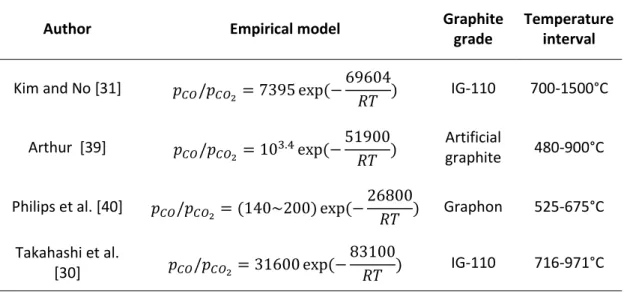
There are several previous studies that have constructed empirical models for predicting the fraction between produced carbon monoxide and carbon dioxide in respect to temperature when oxidizing graphite. The empirical models and their temperature intervals is displayed in Table 2.

Table 2: Empirical models for the fraction between carbon monoxide and carbon dioxide in the off-gas when oxidizing graphite.

Author Empirical model Graphite

grade

Temperature interval

Kim and No [31] 𝑝_𝐶𝑂/𝑝_𝐶𝑂2= 7395 exp(−69604

𝑅𝑇 ) IG-110 700-1500°C Arthur [39] 𝑝_𝐶𝑂/𝑝_𝐶𝑂2 = 103.4_exp(−51900

𝑅𝑇 )

Artificial

graphite 480-900°C Philips et al. [40] 𝑝_𝐶𝑂/𝑝_𝐶𝑂2= (140~200) exp(−26800

𝑅𝑇 ) Graphon 525-675°C Takahashi et al.

[30] 𝑝𝐶𝑂/𝑝𝐶𝑂2= 31600 exp(− 83100

𝑅𝑇 ) IG-110 716-971°C

In a study conducted by Philips et al. [40] the fraction of carbon monoxide and carbon dioxide was investigated. Graphite oxidation experiments were conducted on the graphite grade graphon and a mass spectrometer was used to measure the partial pressure of oxygen, carbon monoxide and carbon dioxide in the temperature interval 525-675°C with oxygen pressures between 10-200

15

millitorr. It was concluded that the kinetic pre-exponential factor was a function of the degree of burn-off and of the concentration of surface oxides complexes. It was also concluded that the fraction of carbon monoxide and carbon dioxide in the off-gas is dependent on the surface oxide complexes content on the graphite surface.

1.3 Mathematical and CFD-modeling of graphite oxidation

There are some previous studies that have used results from graphite oxidation experiments and fundamental theories to construct mathematical models. Those models have later been benchmarked by using numerical simulations. These numerical simulations were conducted with the use of computational fluid dynamics software’s or by using numerical methods in order to solve multi-dimensional flows, mass transport and heat transport equations. [41][42]

As mentioned earlier, graphite oxidation is a complex phenomenon. In order to make an accurate model of this phenomenon a large number of different parameters needs to be known. Some of those includes molecular diffusion rate of oxygen in graphite, activation energies for the reactions, surface active sites, impurities effect etc. [19]

The oxidation mechanism for the reaction between oxygen and carbon needs to be addressed properly in order to build a proper graphite oxidation model. Despite the extensive work done in the field of graphite oxidation there are still diverse views on the primary oxidation steps, since the oxidation mechanism is complex and that the reaction rate depends on many factors. The modelling of such a reaction mechanism requires extensive knowledge of different types of parameters and their effect on the oxidation. Important kinetic parameters such as activation energies and order of reaction can be found in previous experimental studies. [19] [43]

In study made by El-Genk et al. [19] a numerical approach was suggested and a mathematic model constructed in order numerically simulate graphite oxidation. The mathematical model was benchmarked against several previous oxidation experiments on the graphite grades NGB-18 and IG-110. El-Genk et al. suggested that the activation energy for the desorption of carbon atoms from the basal planes of the graphite are not constant but it follows a normal distribution function. The main reason for this is due to the produced organic surface oxide complexes such as alcohols, ethers and ketones etc which have different affinities to oxygen. Four governing graphite oxidation equations were suggested which describes the transport of oxygen In this mathematical model, important phenomena’s were taken in to account such as the burn-off degree and change in ASA over time. The model was benchmarked against experimental data. The model was tested by using the numerical software Matlab and the commercial CFD-software Star-ccm+. The model displayed a good match to the experimental result of the previous oxidation experiments.

Other studies has been conducted where CFD-models, created from commercial CFD-software’s, were benchmarked against controlled graphite oxidation experiments [44]. Amongst these studies there are some who used commercial CFD-software’s to simulate the event of air ingress accidents in a high temperature gas-cooled reactor (HTGR) in the nuclear energy field. Graphite oxidation, during air ingress accidents, is an important factor since it can result in damage of the interior reactor and thus result in shortage in expected reactor lifetime. In a study conducted by Kadak and Zhai [45] , the commercial CFD-software Fluent was benchmarked against several air ingress experiments conducted by the Japanese atomic energy research institute (JAERI) and by the Julius research center in Germany at the NACOK facility, where NACOK stands for “Naturzug Im Core Mit Korrosion” [46] [47]. The output data from the numerical simulations regarding the off-gas composition over time matches that of the experimental result to a high degree. The main gas compounds of the off-gas consisted of residual oxygen, helium, nitrogen, carbon monoxide and carbon dioxide. The gas

16

compounds of the off-gas were measured as mole fraction over time. Kadak and Zhai [45] were able to show that the commercial CFD-software Fluent could successfully be used to numerically simulate the different phenomena or events in air ingress accidents. The numerical simulations results regarding the experiments conducted at NACOK facility also displayed a good match between the experimental data and the output data obtained from the numerical simulations.

In a study by Ferng and Chi [48] , a CFD-model was constructed in order to simulate air ingress phenomena in a HTGR. Although, this study focused on the graphite oxidation of the high-temperature reactor core. The commercial CFD-software Fluent was used as the numerical tool to investigate the oxidation distribution within a high temperature reactor core

A study which involved both graphite oxidation experiments and a numerical simulations were conducted by Kim and No [31]. Graphite oxidation experiments were conducted on the graphite grade IG-110 over a wide temperature interval, 700-1500°C, and with various oxygen concentrations. From the graphite oxidation experiments kinetic parameters such as activation energy and order of reaction were determined. The concentrations of the produced carbon monoxide and carbon dioxide were monitored and an empirical model of the fractions between as a function of the temperature were obtained. A numerical model was constructed by using commercial CFD-software Fluent in order to determine the initial graphite oxidation rate at zero burn-off degree. The experimentally obtained kinetic-parameters and the fraction between carbon monoxide and carbon dioxide were used as input data in the numerical simulations. The output data from the numerical simulations matched the experimental results to a high degree. A semi-empirical model, based on the experimental results, was also suggested.

A blind benchmarking of the air ingress experiments from NACOK experimental facility in Germany was conducted by Brudieu. [49] The main goal of this study was to examine the commercial CFD-software Fluent ability to simulate the phenomenon of natural convection, graphite oxidation and distribution of heat generated by the exothermal reactions etc in a HTGR. A parameters study were conducted regarding reaction kinetics, solver, mesh and fluid flow etc in order to find the most suitable numerical model.

Similar numerical treatments of the graphite oxidation studies of the JAERI and NACOK experiments were conducted by Zhai [50] and by Lim and No [51].

17

1.4 Previous studies regarding the experimental setup for oxidation experiments

Graphite oxidation has been extensively researched by previous studies. In this part of the study, emphasis was made to review experimental methods which has been used by previous studies to conduct graphite oxidation experiments where it were possible to control the temperature, mass loss/mass loss rate over time and furnace atmosphere.

Many of the reviewed previous studies are related to graphite oxidation in nuclear energy industry, see Table 3.

Table 3: Previous experimental studies regarding graphite oxidation.

Author Graphite grade Sample shape and mass Sample dimensions Experimental apparatus Gas Gas flow rate Temperature Sharma et al. [32] 110, IG-430, NBG-18 and NBG-25 Shape not specified Mass: 10-12mg Not specified TGA Q500 IR Air and oxidizing gas (10%O2 90% N2) At least 40 mL/min From RT to 800°C Guldbransen et al. [37] Graphite (AGKSP) Cylinder Mass: 0.050g ∅𝑑 3.2 mm ℎ: 3.9 mm Author designed apparatus + Mass spectroscopy Air and commercial grade oxygen For Oxygen approx. 9.1-431 mL/min 1200-1524°C Windes and Smith [52] Not mentioned Cylinder Mass: not specified ∅𝑑 25.4 mm ℎ: 50.8 mm Vertical tube furnace (ASTM 7542) Air 10 L/min 750°C Xiaowei et al. [28] IG-11 Cylinder Mass: 1.7g ∅𝑑 10 mm ℎ: 10 mm TGA TA2000C Mettler Dry air 20 mL/min 400-1200°C Smith [53] NBG-18 and PCEA Cylinder Mass: not specified ∅𝑑 25.4 mm ℎ: 50.8 mm Vertical tube furnace (ASTM D7542-09) Air and Helium 10 L/min 750°C Fuller and Okoh [33] IG-110 Cylinder Mass: 1.756g ∅𝑑 0.838 cm ℎ: 1.905 mm TGA Mettler model TA1 serial #61 Dry air 0.496-0.500 L/min 450-750°C Hong and Chi [29] 11, IG-110 and IG-430 Cylinder Mass: approx. 0.4320g ∅𝑑 2.54 cm ℎ: 2.54 cm Vertical tube

furnace Dry air 4 L/min 600-900°C

Payne et al. [22] PGA Cube Mass: Not specified (4 𝑚𝑚)3 Mettler _Toledo TGA/DCS Nitrogen and Air 25 mL/min 600-1150°C

18

There are several more previous studies which also utilize the thermogravimetric analysis (TGA) for studying graphite oxidation than what is displayed in Table 3, see also [13], [25] , [28] and [27].

1.4.1 Thermogravimetric analysis

The thermogravimetric analyzer (TGA) is an experimental apparatus used in various research fields. The TGA is used in fields related to thermal analysis, the study of how material properties change with temperature. [54]

The basic principle of the TGA is that it continuously measures the weight of a sample as it is subjected to either non-isothermal or isothermal heat treatments in an inert or reactive atmosphere. The main output data of the TGA is the weight change and rate of weight change as function of time or temperature. The weight loss during certain experimental conditions relates to different chemical and physical phenomena’s that occurs in the material during the experimental procedure. Some examples of phenomena’s that are investigated by using the TGA are given in Table 4.

Table 4: Different phenomena which causes mass changes. [55]

TGA

Physical Chemical

Phase transitions Decomposition

Gas adsorption Break down reactions

Gas desorption Gas reactions (oxidation etc)

Vaporization Chemisorption

Sublimation

By using the TGA, kinetic parameters such as activation energy and the order of reaction can be measured. The TGA is also used to characterize thermal stability, material purity and determination of humidity in a material. The usage of TGA can be found in areas related to corrosion, gasification or kinetic studies. [55][56]

There are different arrangements found in commercial TGA, the TGA can may be constructed differently depending on manufacturer. There are both vertical and horizontal TGA found in market. The TGA is in principal the combination of a heating furnace together with a sensitive digital scale. The temperature in the furnace is usually measured by an outer- and an inner thermocouple. Inert or reactive gas can be injected into the furnace chamber by a gas inlet which is located at the bottom part or the top part of the furnace. The sample is connected to the digital scale by a wire or a cage consisting of inert and high temperature resisting material. The furnace is connected to an electrical power control station while the digital scale is connected to a computer which monitors and stores the weight changes obtained by during the experiment. The schematics of a vertical TGA is displayed in Figure 10.

Depending on the manufacturer and type of furnace, a TGA could reach temperatures from room temperature up to 2000°C with programmable heating rates. The sample size used in the TGA can vary in both geometry and weight. The geometry can be cylindrical, cubic to spherical and the weight can vary from micrograms to grams depending on the sensitivity of the digital scale.

19

Figure 10: The general schematics of a vertical TGA. [57]

The experimental procedure may differ depending on the type of study. The general procedure of an isothermal oxidation experiment can be seen below in steps 1-4. [22]

1) Calibration of the digital scale by using an identical test sample instead of the actual sample to identify the effect of the incoming gas flow momentum on the digital scale. When this is completed and corrected, the test sample is replaced by the actual sample.

2) Gas injection of inert gas or a vacuum pump is used is to remove all the air inside the furnace. When the air has been removed, a constant heating rate is used to obtain the relevant furnace temperature. Inert gas is injected to uphold the inert atmosphere.

3) Once the experimental temperature is obtained, the experimental temperature is held constant. Inert gas is turned off and the reactive gas is turned on.

4) When sufficient weight loss is obtained or a specific pre-determined time period has elapsed, the experiment is complete and the reactive gas is switched over to inert gas and the furnace is cooled with a constant cooling rate.

20

1.4.2 The graphite oxidation experiment by Kim and No [31]

As mentioned earlier, Kim and No [31] conducted both graphite oxidation experiments and numerical CFD-simulations. The study was conducted in order to investigate graphite oxidation related to the air ingress of a HTGR. The study was conducted by experimentally investigating the impact of parameters such as oxygen concentration and temperature on the initial graphite oxidation rate. [31]

The experimental setup and experimental apparatus, which were used to conduct the graphite oxidation experiments, are displayed in Figure 12.

T [°C] W [%] t [𝑚𝑖𝑛] t [𝑚𝑖𝑛] RT 100 % % 2) 3) 4)

Figure 11: The schematics of a general isothermal TGA procedure. The upper plot displays the temperature versus time while the lower plot displays the weight versus time.

Inert gas

Constant heating rate Te

Reactive gas Constant temperature

Inert gas

21

Figure 12: The experimental setup and experimental apparatus from the oxidation experiment of Kim and No [31].

Since the study were investigating graphite oxidation related to air ingress in a HTGR a gas mixture of helium and oxygen, helium is normally used as coolant in a HTGR. The oxygen concentration in the gas mixture varied from 2.5-20vol%. As can be seen in Figure 12, the gas mixtures are obtained by mixing helium and oxygen from separate gas tanks and the gas flow rate was controlled by two separate mass flow controllers. The desired gas mixture was then injected into a cylindrical quartz tube from the bottom inlets. The cylindrical graphite sample was installed between two cylindrical ceramic rods. An induction heater was placed around the cylindrical quartz tube in the area where the graphite sample was located. The induction heater then heated the graphite sample to temperatures between 700-1500°C and the surface temperature of the graphite was monitored by a non-contact infrared thermometer, see Figure 13.

22

An off-gas analyzer was also used in order to measure the off-gas composition. From the carbon monoxide and carbon dioxide concentrations in the off-gas the graphite oxidation rate could be calculated.

The experimental procedure was the following.

A) Pure helium gas was injected into the cylindrical quartz tube to remove all atmospheric gases.

B) When the oxygen concentration in the cylindrical quartz tube has reached zero, the induction heater was turned on and the graphite sample was heated to the desired temperature. C) When the graphite surface temperature became stable, the desired gas mixture was injected

through the inlets of the cylindrical quartz tube.

D) The off-gas composition was continuously measured by the gas analyzer and provided data which were used to calculate the graphite oxidation rate for a specific temperature and oxygen concentration. The ratio between the carbon monoxide and carbon dioxide for each temperature was also calculated from the off-gas analysis.

The experimental parameters which were used as variables for the graphite oxidation experiment can be seen in Table 5.

Table 5: The variable parameters in the oxidation experiment. STLPM means standard liters per minuets.

Gas flow rate [STLPM] Oxygen concentration [vol%] Temperature [°C]

40 2.5 % , 5%, 10% and 20 % 700-1500

2 Method

2.1 Suggesting experimental apparatus and setup

In order to determine which experimental apparatus and setup that were best suited in providing the needed experimental data, for the benchmarking of the dynamic coupling approach, some basic requirements were set.

The experimental apparatus and setup should be able to:

1) Provide continuous information regarding the sample mass loss over time and the sample mass loss rate.

2) Control parameters such as temperature and furnace atmosphere. 3) Conduct isothermal experiments.

4) Use and inject gases into the furnace with a controlled mass flow rate. 5) Use a simple furnace geometry.

23

2.2 Numerical setup

The commercial CFD-software used for the numerical simulations was Fluent version 15.0. The commercial CFD-software was used on a computer with Windows 8.1 Enterprise and the following system, see Table 6.

Table 6: The computer system used to run the numerical simulations in this study.

Computer system

Processor Intel® Core™ i7-5930K CPU@

3.50 GHz

Memory 32.0 GB

System type 64-bit Operating System,

x64-based processor

The numerical simulations were used to benchmark Fluent against the graphite oxidation experiments conducted by Kim and No. A parameter study was also conducted testing the effect of the mass diffusion conditions, gas flow rate and the kinetic parameters on the numerically calculated graphite oxidation rate at zero burn-off degree.

2.2.1 Computational domain and mesh

For the numerical simulations, a 3D-model was selected which was similar to the experimental apparatus used by Kim and No, see Figure 14. The length of the cylindrical quartz tube was approximated since no information was given regarding the length of the tube. The same were applied for the exact position of the graphite specimen. The used dimensions can be seen in Table 7.

Figure 14: The computational domain for the numerical simulations. In the image to the left the outer domain is visible. The image to the right displays the ceramic tube surface and graphite location.

Graphite location Outlet Inlet L D h d H

24 Table 7: The dimensions of the computational domain

Dimensions Value [cm] L 50 D 7.6 d 3 h 2.1 H 35

The inner parts of the cylindrical ceramic tube volume and graphite sample were not taken into account as a part of the computational domain. Only the fluid part and the graphite sample surface were taken into account as a part of the computational domain in the numerical simulations.

The mesh used for the numerical simulation can be seen in Figure 15.

Figure 15: The mesh of the computational domain. The left image displays the whole tube and the right image displays the mesh surface

A symmetric quadrilateral structured mesh was used in order to obtain high accuracy in the inner part of the computational domain. The number of nodes, elements and the size limitations of the elements can be seen in Table 8.

Table 8: Mesh specifications used for the numerical simulations.

Mesh parameters Value

Nodes 34580

Elements 80898

Maximum size 2.5∗ 10−2 [m]

Minimum size 1.25∗ 10−4 [m]

2.2.2 Surface reaction model and governing equations

In Fluent 15.0 there was an option for applying reactions and species transport in flows or at surfaces. The governing transport equations which was used for species transport in Fluent can be seen in equation 1. [59] 𝜕 𝜕𝑡(𝜌𝑌𝑖) + 𝜕 𝜕𝑥𝑗(𝜌𝑢𝑗𝑌𝑖) = 𝜕 𝜕𝑥𝑗(𝜌𝐷𝑖 𝜕𝑌𝑖 𝜕𝑥𝑗) + 𝑅𝑖+ 𝑆𝑖 (1)

25 𝜌: Density.

𝑌_𝑖: Mass fraction for chemical species 𝑖. 𝐷_𝑖: Diffusion coefficient.

𝑅_𝑖: Reaction source term.

𝑆_𝑖: Other types of source terms beside the reaction.

The reaction source term 𝑅𝑖 is the sum of all the reaction sources over the amount of reactions which species 𝑖 participate in, see equation 2.

𝑅_𝑖 = 𝑀_𝑤,𝑖∑ 𝑟_𝑖,𝑛

𝑁𝑅

𝑛=1

(2)

𝑀𝑤,𝑖: Molecular weight of species 𝑖.

𝑟_𝑖,𝑛 : The molar rate of creation or breakdown of species 𝑖.

In the numerical simulations, the laminar finite-rate model was used due to the assumption that graphite oxidation follows the reaction kinetics described by an Arrhenius expression, the reaction source term was based on Arrhenius kinetics.

According to the Ansys Fluent theory guide [59], a general chemical reaction, in Fluent, was computed as seen in equation 3. [59]

∑ 𝑣_𝑖,𝑛′ _𝑀 𝑖 𝑘𝑓,𝑛 ↔ 𝑘𝑏,𝑛 𝑁 𝑖=1 ∑ 𝑣_𝑖,𝑛′′ _𝑀 𝑖 𝑁 𝑖=1 (3)

𝑁: Number of chemical species in the system. 𝑀_𝑖: Symbol denoting a species 𝑖.

𝑣_𝑖,𝑛′ _{: Stoichiometric coefficient for reactant 𝑖 in reaction 𝑛.} 𝑣_𝑖,𝑛′′ _{: Stoichiometric coefficient for the product 𝑖 in reaction 𝑛.} The molar reaction rate for species 𝑖 is given by equation 4.

𝑟𝑖,𝑛= ∑ 𝛾𝑗,𝑛𝐶𝑗 𝑁𝑛 𝑗 ∗ (𝑣𝑖,𝑛′′ − 𝑣𝑖,𝑛′ ) ∗ (𝑘𝑓,𝑛∏|𝐶𝑗,𝑛|𝑛𝑗,𝑛 ′ 𝑁𝑛 𝑗=1 − 𝑘𝑏,𝑛∏|𝐶𝑗,𝑛|𝑛𝑗,𝑛 ′′ 𝑁𝑛 𝑗=1 ) (4)

𝑁_𝑛: Number of chemical species in the reaction 𝑛.

𝐶𝑗,𝑛: Molar concentration of each reactant and product species 𝑗 in reaction 𝑛. 𝑛_𝑗,𝑛 ′ : Forward rate exponent for each reactant product species 𝑗 in reaction 𝑛. 𝑛_𝑗,𝑛 ′′ _{: Backward rate exponent for each reactant and product species 𝑗 in reaction 𝑛}

26

𝛾_𝑗,𝑛: Third-body efficacy of the 𝑗: 𝑡ℎ species in the 𝑛: 𝑡ℎ reaction.

The forward reaction rate constant for reaction 𝑛 was expressed by an expanded version of the Arrhenius expression, see equation 5.

𝑘𝑓,𝑛= 𝐾𝑟𝑇𝛽𝑟exp (− 𝐸

𝑅𝑇) (5)

𝐾_𝑟: Pre-exponential factor 𝐸: Activation energy 𝑅: Universal gas constant 𝑇: Absolute temperature 𝛽_𝑟: A temperature exponent.

The backward reaction rate constant was obtained by using the relationship between the forward reaction rate and the thermodynamic equilibrium constant, see equation 6 and equation 7. [59]

𝑘𝑏,𝑛= 𝑘𝑓,𝑛 𝐾 (6) and 𝐾 = exp (∆𝑆𝑟 𝑅 − ∆𝐻𝑟 𝑅𝑇) ( 𝑝𝑎𝑡𝑚 𝑅𝑇 ) ∑𝑁_𝑖=1(𝑣_𝑖,𝑟′′−𝑣_𝑖,𝑟′ ) (7)

∆𝑆_𝑟: The change in entropy for free unmixed reactants and products at standard condition.

∆𝐻_𝑟: The change in entropy and enthalpy for free unmixed reactants and products at standard condition.

𝑝𝑎𝑡𝑚: The atmospheric pressure.

There are two types of reactions available in Fluent, volumetric- and surface reactions. For volumetric reactions, the rate of reactions is simply included in the species transport equation, see equation 1, as reaction source terms. For surface reactions, the rate of reactions is dependent on the rate of adsorption and the rate of desorption as well as the mass diffusion of the reactants and products to and away from the reactive surface, which implies the need of several more source terms than for volumetric reactions. [59]

A general wall surface reaction, includes gas species, solid species and the surface-adsorbed species can be seen in equation 8.

∑ 𝑔_𝑖,𝑛′ 𝐺𝑖 𝑁𝑔 𝑖=1 + ∑ 𝑏_𝑖,𝑛′ 𝐵𝑖 𝑁𝑏 𝑖=1 + ∑ 𝑠_𝑖,𝑛′ 𝑆𝑖 𝑁𝑠 𝑖=1 𝑘𝑓 → ∑ 𝑔_𝑖,𝑛′′ 𝐺𝑖 𝑁𝑔 𝑖=1 + ∑ 𝑏_𝑖,𝑛′′ 𝐵𝑖 𝑁𝑏 𝑖=1 + ∑ 𝑠_𝑖,𝑛′′ 𝑆𝑖 𝑁𝑠 𝑖=1 (8) 𝐺_𝑖: Gas species. 𝐵_𝑖: Solid species. 𝑆𝑖: Site species.

27 𝑁_𝑔: Total sum of gas species.

𝑁_𝑏: Total sum of solid species. 𝑁𝑠: Total sum of site species.

It was not possible to take into account reversible reactions in Fluent surface reaction model, only the forward reaction constants,𝑘𝑓, were used. The reaction rate is determined by the using rate law for surface reactions, see equation 9.

𝑅_𝑟 = 𝑘_𝑓(∏[𝐶_𝑖]_{𝑤𝑎𝑙𝑙}𝑛𝑖,𝑔,𝑛′ 𝑁𝑔 𝑖=1 ) (∏[𝑆𝑗]_{𝑤𝑎𝑙𝑙}𝑛𝑖,𝑔,𝑛 ′ 𝑁𝑠 𝑗=1 ) (9)

[𝐶𝑖]: Site species on the wall surface

Other governing equations, besides for the species transport displayed in equation 1, and physical property equations ,which were used in the numerical simulation, are listed below, see equations 10-24.

The mass conservation equation

𝜕𝜌

𝜕𝑡+ ∇ ∙ (𝜌𝑣⃑) = 𝑆𝑚 (10)

𝑆_𝑚: Source term of the mass added from a second dispersed term.

The momentum equation

𝜕 𝜕𝑡(𝜌𝑣⃑) + ∇ ∙ (𝜌𝑣⃑𝑣⃑) = ∇p + ∇ ∙ (𝜏⃑) + 𝑝𝑔⃑ + 𝐹⃑ (11) and 𝜏⃑ = 𝜇 [(∇𝑣⃑ + ∇𝑣⃑T_{) −}2 3∇ ∙ 𝑣⃑I] (12) 𝑣⃑: Velocity vector. p: Static pressure. 𝜇: Molecular viscosity. 𝜏⃑: Stress tensor. I: Unit tensor.

The energy equation

𝜕

28 𝐸: Energy.

𝑘_𝑒𝑓𝑓: Effective thermal conductivity.

𝑆ℎ: Source term which contains the energy contributions due to radiation. The equations for the physical properties is displayed below.

Heat capacity

𝐶_𝑝= ∑ 𝑌_𝑖𝐶_𝑝,𝑖 𝑖

(𝑀𝑖𝑥𝑖𝑛𝑔 𝑙𝑎𝑤) ₍₁₄₎

𝑌_𝑖: Mass fraction of each species.

𝐶_𝑝,𝑖: Individual heat capacity for each species.

Density 𝜌 = _𝑅𝑃𝑜𝑝 𝑀_𝑤𝑔𝑇 (𝑖𝑛𝑐𝑜𝑚𝑝𝑟𝑒𝑠𝑠𝑖𝑏𝑙𝑒 𝑖𝑑𝑒𝑎𝑙 𝑔𝑎𝑠) (15) 𝑃_𝑜𝑝: Operational pressure. 𝑀_𝑤𝑔: Gas molecular mass.

Viscosity 𝜇 = ∑ 𝑋𝑖𝜇𝑖 ∑ 𝑋𝑗 𝑖𝜑𝑖,𝑗 𝑖 (𝐼𝑑𝑒𝑎𝑙 𝑔𝑎𝑠 𝑚𝑖𝑥𝑖𝑛𝑔 𝑙𝑎𝑤) ₍₁₆₎ And 𝜑𝑖,𝑗= [1 + (𝜇𝑖 𝜇_𝑗) 0.5 (𝑀_𝑀𝑤,𝑗 𝑤,𝑖) 0.25 ] [8 (1 +𝑀_𝑀𝑤,𝑖 𝑤,𝑗)] (17)

𝑋_𝑖: Mole fraction of species 𝑖.

Thermal conductivity

𝑘 = ∑ 𝑌𝑖𝑘𝑖 𝑖

29 𝑘_𝑖: Thermal conductivity for species 𝑖.

Mass diffusion 𝐽_𝑗 ⃑⃑⃑ = − ∑ 𝜌𝐷_𝑖𝑗∇𝑌_𝑗 𝑁−1 𝑗=1 (𝑀𝑎𝑥𝑤𝑒𝑙𝑙 − 𝑆𝑡𝑒𝑓𝑎𝑛 𝑒𝑞𝑢𝑎𝑡𝑖𝑜𝑛) (19)

𝐷𝑖𝑗: Binary gas-phase diffusion coefficient. 𝐽𝑗

⃑⃑⃑ : Diffusive mass flux vector.

𝐷_𝑖𝑗 = [𝐷] = [𝐴]−1_{[𝐵] (20)} And 𝐴_𝑖𝑖 = − ( 𝑋𝑖 𝐷_𝑖𝑁 𝑀_𝑤 𝑀_𝑤,𝑖+ ∑ 𝑋_𝑖 𝐷_𝑖𝑗 𝑁 𝑗=1 𝑗≠𝑖 𝑀_𝑤 𝑀_𝑤,𝑖 ) (21) 𝐴_𝑖𝑗 = −𝑋_𝑖(1 𝐷_𝑖𝑗 𝑀𝑤 𝑀_𝑤,𝑗+ 1 𝐷_𝑖𝑁 𝑀𝑤 𝑀_𝑤,𝑁) (22) 𝐵𝑖𝑖 = − (𝑋𝑖 𝑀_𝑤 𝑀𝑤,𝑁+ (1 − 𝑋𝑖) 𝑀_𝑤 𝑀𝑤,𝑖) (23) 𝐵_𝑖𝑗= −𝑋_𝑖(𝑀𝑤 𝑀_𝑤,𝑗− 𝑀_𝑤 𝑀_𝑤,𝑁) (24)

The binary gas-phase diffusion coefficients for the gas compounds were calculated by using the empirical equation suggested by Fuller et al. [60], see equation 25.

𝐷_𝑖𝑗=

10−7_𝑇1.75_[(𝑀𝑖+ 𝑀𝑗) 𝑀𝑖𝑀𝑗 ] 𝑃 (𝜎13_𝑖+ 𝜎13_𝑗)

2 (25)

By conducting a Taylor expansion on equation 25, equation 26 was obtained. 𝐷_𝑖𝑗= 𝐶₁+ 𝐶₂𝑇 + 𝐶₃𝑇2_{+ 𝐶}

4𝑇3+ 𝐶5𝑇4 (26)