THESIS
ANALYSIS OF CONTAMINANT MASS IN PLACE IN TRANSMISSIVE AND LOW-K ZONES
Submitted by
Eric Roads
Department of Civil and Environmental Engineering
In partial fulfillment of the requirements
For the Degree of Master of Science
Colorado State University
Fort Collins, Colorado
Summer 2020
Master’s Committee: Advisor: Tom Sale Sybil Sharvelle Sally Sutton
Copyright by Eric Michael Roads 2020 All Rights Reserved
ABSTRACT
ANALYSIS OF CONTAMINANT MASS IN PLACE IN TRANSMISSIVE AND LOW-K ZONES
Contaminant hydrology has been challenged by the common perception of homogeneous subsurface media. Previous sampling methods neglect the importance of differentiating between transmissive and low-k zones. Cryogenic core collection is a high-resolution sampling technique that can highlight the occurrence of transmissive and low-k zones as well as the distribution of contaminants in transmissive and low-k zones. Cryogenic core collection uses a CSU patented process that preserves core samples downhole using liquid nitrogen. Frozen cores are shipped to CSU on dry ice and always kept at -80° C. Cores are cut into subsamples and analyzed to
determine geology, physical properties, contaminant concentrations, and microbial ecology. The data is processed into Excel™ and then stored in gINT™, a relational database. Herein,
consideration is given to 390 feet of collected core from 31 boreholes from 5 hydrocarbon and 2 chlorinated solvent sites. Data analyses include comparisons within a site, intra-site
comparisons, and between sites, inter-site comparisons.
Tools are developed in gINT™ to automate transformation of collected data into vibrant visual graphical outputs. First, for every borehole, a graphic is generated that includes a
comprehensive panel of geology, contaminants of concern and fluid saturations properly
presented by depth. Building on this, distributions of contaminants as a function of transmissive or low-k zones are resolved. Lastly, key attributes of mass distribution are compared across
Our analysis presents a first-ever quantification of distribution of contaminant mass in transmissive and low-k zones. The analysis begins with processing concentration data-by-depth to produce the total mass of contaminants in each borehole, the mass of contaminants in
transmissive zones, and the mass of contaminants in low-k zones. The contaminant mass in a borehole is presented for each contaminant individually and as sum of all contaminants. The visualization of this data is not intuitive due to the ranges of contaminant mass in place. Hydrocarbons contaminated sites have contaminant masses that range from less than half a kilogram to about 30 kilograms of contaminants per m2. Chlorinated solvent contaminated sites have contaminant masses that vary from less than 240 micrograms to right under 2.5 kilograms of contaminants per m2.
The data is processed such that boreholes and sites with broad ranges of conditions can be compared. Data is presented as percent of contaminant mass in transmissive zones by borehole; the percent of contaminant mass in low-k zones by borehole, the percent of borehole that is transmissive, and percent of borehole that is low-k. Unlike previous data that required a y-axis formatted to a log scale, this data is visualized on a plot with the y-axis set at 0-100%. The fraction of a borehole that is low-k ranges between 0% and 94% with a median value of 52%. Secondly, the fraction of total contaminant mass stored in low-k zone ranges from 1% to 96% with a median value of 46%.
Illustrations of the tendency for mass storage in low-k zones are presented through
difference in percent of borehole that is low-k and percent of contaminants in a borehole in low-k zones. The calculations defined a positive difference as preference for transmissive zones and a negative difference as preference for low-k zones. Data presented characterized the 18
hydrocarbon contaminated boreholes, 12 chlorinated solvent contaminated boreholes, and all 30 contaminated boreholes respectively. Key insights include
• Hydrocarbon contaminated boreholes showed statistically significant preference for low-k zones if the unit difference of percent of borehole that is low-k and percent of contaminants in a borehole in low-k zones was less than -24%. • Chlorinated solvent contaminated boreholes showed statistically significant
preference for low-k zones if the unit difference of percent of borehole that is lowk and percent of contaminants in a borehole in lowk zones was less than -11%.
• Remediated chlorinated solvent boreholes presented a preference for low-k zones where their non-remediated counterparts showed preference for transmissive zones..
• All contaminated boreholes showed statistically significant preference for low-k zones if the unit difference of percent of borehole that is low-k and percent of contaminants in a borehole in low-k zones was less than -19%.
• As an example, this thesis provides a unique documentation of benezene
persisting in low-k zones. The presesnce or absensce of benzene in low-k zones will have a large implication with respect to the longeviety of benzene in
monitoring wells and the efficacy of remedial measures that address the longevity of benzene in monitoring wells.
Overall, cryogenic core collection and advanced analytics provides a practical means of
ACKNOWLEDGEMENTS
Primary funding for this work came from sponsors of the University Consortium for Field Focus Groundwater Research including Chevron, ExxonMobil, and BP.
Special thanks to my advisor, Dr. Tom Sale, and committee members, Dr. Sharvelle and Dr. Sutton. Also, special thanks to my family and friends, especially my wife and parents who have been there for me through everything. I could not have finished this program without their help and support.
The data presented in this thesis was not collected or directly analyzed by the author but by members of the CCH team over many years. My primary contribution is organizing and provided methods for furthering analysis of contaminants in transmissive and low-k zones. Thus, it is very important that other individuals are acknowledged for their contributions. The following table summarizes each Site and the main contributors.
Site Collection Visual Analysis Lab Analysis
A Rick Johnson Tom Sale & Eric
Roads
Maria Irianni-Renno & Eric Roads
B Maria Irianni-Renno
& Tom Sale,
Tom Sale & Eric Roads
Maria Irianni-Renno & Eric Roads
C Tom Sale Tom Sale Maria Irianni-Renno
D Tom Sale Tom Sale Maria Irianni-Renno
E Tom Sale & Maria
Irianni-Renno
Tom Sale Maria Irianni-Renno
F Rick Johnson & Tom
Sale
Tom Sale Mitch Olson,
G Rick Johnson &Tom
Sale,
TABLE OF CONTENTS
ABSTRACT ... ii
ACKNOWLEDGEMENTS ... v
LIST OF TABLES... ix
LIST OF FIGURES ... xi
LIST OF EQUATIONS ... xiii
CHAPTER 1: INTRODUCTION & PROBLEM STATEMENT ... 1
1.1 Background Information ... 1
1.2 Objectives ... 6
1.3 Organization and Content ... 7
CHAPTER 2: METHODS ... 8
2.1 Sites ... 8
2.1.1 Site A... 10
Use and COC ... 10
Depositional Environment ... 10
Core Collection ... 10
2.1.2 Site B... 10
Use and COC ... 10
Depositional Environment ... 11
Core Collection ... 11
2.1.3 Site C ... 11
Use and COC ... 11
Depositional Environment ... 12
Core Collection ... 12
2.1.4 Site D ... 12
Use and COC ... 12
Depositional Environment ... 12
Core Collection ... 12
2.1.5 Site E... 13
Core Collection ... 13
2.1.6 Site F and Site G ... 13
Use and COC ... 13
Depositional Environment ... 14
Core Collection ... 14
2.1.7 Site H ... 15
Use and COC ... 15
Depositional Environment ... 15
Core Collection ... 15
2.2 Core Collection and Processing ... 16
2.2.1 Core Collection ... 16
2.2.2 Core Processing: Overview of Steps ... 16
2.2.3 Core Processing: Cutting plan... 17
2.2.4 Core Processing: Cutting ... 18
2.2.5 Core Processing: Sample Preservation ... 19
2.3 Sample analysis ... 22
2.3.1 Visual ... 22
2.3.2 COC ... 23
2.3.3 Microbial ... 23
2.4 Data Analysis ... 23
2.4.1 Database: Need for gINTä and Use of Excelä ... 23
2.4.2 Database: Standardization ... 24
2.4.3 Analytical: Transmissive – Low k ... 25
2.4.4 Analytical: Total Mass in Place in Borehole, Transmissive Zones, and Low-k Zones ... 27
2.4.5 Analytical: Fraction of Primary COC in Transmissive and Low-k Zones... 29
2.4.6 Analytical: Intra-Site and Inter-Site Comparison ... 32
CHAPTER 3: RESULTS ... 33
3.1 Intra-Site Analysis... 33
3.1.1 Intra-Site A ... 33
3.1.1.1 Contamination by Depth ... 34
3.1.1.2 Mass in Place Summary Analysis ... 47
3.1.2.1 Contamination by Depth ... 54
3.1.2.2 Mass in Place Summary Analysis ... 65
3.1.2.3 Mass in Transmissive and Low-k Zones Summary Analysis... 65
3.1.3 Intra-Site C ... 70
3.1.3.1 Contamination by Depth ... 70
3.1.3.2 Mass in Place Summary Analysis ... 74
3.1.3.3 Mass in Transmissive and Low-k Zones Summary Analysis... 75
3.1.4 Intra-Site D ... 79
3.1.4.1 Contamination by Depth ... 79
3.1.4.2 Mass in Place Summary Analysis ... 82
3.1.4.3 Mass in Transmissive and Low-k Zones Summary Analysis... 83
3.1.5 Intra-Site E ... 87
3.1.5.1 Contamination by Depth ... 87
3.1.5.2 Mass in Place Summary Analysis ... 88
3.1.5.3 Mass in Transmissive and Low-k Zones Summary Analysis... 89
3.1.6 Intra-Site F ... 93
3.1.6.1 Contamination by Depth ... 93
3.1.6.2 Mass in Place Summary Analysis ... 99
3.1.6.3 Mass in Transmissive and Low-k Zones Summary Analysis... 99
3.1.7 Intra-Site G ... 102
3.1.7.1 Contamination by Depth ... 103
3.1.7.2 Mass in Place Summary Analysis ... 108
3.1.7.3 Mass in Transmissive and Low-k Zones Summary Analysis... 108
3.1.8 Intra-Site H ... 111
3.1.8.1 Contamination by Depth ... 112
3.1.8.2 Mass in Place Summary Analysis ... 119
3.1.8.3 Mass in Transmissive and Low-k Zones Summary Analysis... 119
3.2 Inter-Site Analysis ... 124
3.2.1 Inter-Site: Hydrocarbon Boreholes ... 124
3.2.1.1 Benzene & PCP ... 125
3.2.1.2 Total Petroleum Hydrocarbons... 130
3.2.2 Inter-Site: Chlorinated Solvent Boreholes ... 142
3.2.2.1 SUM CVOCs... 142
3.2.3 Inter-Site: All Boreholes ... 148
3.2.3.1 SUM COCs ... 148
3.3 Discussion of Limitations ... 154
CHAPTER 4: CONCLUSION ... 156
4.1 Key findings... 156
4.2 Implications for Site Characterization ... 158
4.3 Future Work ... 158
LIST OF TABLES
Table 1: Summary of Sites Included... 9
Table 2: Core Intervals for Site A ... 10
Table 3: Core Intervals for Site B ... 11
Table 4: Core Intervals for Site C ... 12
Table 5: Core Intervals for Site D ... 13
Table 6: Core Interval for Site E ... 13
Table 7: Core Intervals for Site F ... 14
Table 8: Core Intervals for Site G ... 14
Table 9: Core Intervals for Site H ... 15
Table 10 : Description of subsample size, designation, preservation technique, and parameters for each Sample ID ... 21
Table 11: Total Mass of Contaminants at Site A ... 48
Table 12: Mass of PCP and Methane at Site A Divided into Zones ... 52
Table 13: Mass of TPH, GRO, and DRO at Site A Divided into Zones ... 52
Table 14: Percentage of Borehole that is Transmissive of Low-k and Percentage of PCP and Methane Mass in Zones at Site A ... 53
Table 15: Percentage of TPH, GRO, and DRO Mass in Zones at Site A ... 53
Table 16: Total Mass of Contaminants at Site B ... 65
Table 17: Mass of Benzene and Methane at Site B Divided into Zones ... 68
Table 18: Mass of TPH, GRO, and DRO at Site B Divided into Zones ... 68
Table 19: Percentage of Borehole that is Transmissive of Low-k and Percentage of Benzene and Methane Mass in Zones at Site B ... 69
Table 20: Percentage of TPH, GRO, and DRO Mass in Zones at Site B... 69
Table 21: Total Mass of Contaminants at Site C ... 76
Table 22: Mass of Benzene and Methane at Site C Divided into Zones ... 76
Table 23: Mass of TPH, GRO, and DRO at Site C Divided into Zones ... 76
Table 24: Percentage of Borehole that is Transmissive of Low-k and Percentage of Benzene and Methane Mass in Zones at Site C ... 78
Table 25: Percentage of TPH, GRO, and DRO Mass in Zones at Site C... 78
Table 26:Total Mass of Contaminants at Site D... 84
Table 27: Mass of Benzene and Methane at Site D Divided into Zones ... 84
Table 28: Mass of TPH, GRO, and DRO at Site D Divided into Zones ... 84
Table 29: Percentage of Borehole that is Transmissive of Low-k and Percentage of Benzene and Methane Mass in Zones at Site D ... 86
Table 30: Percentage of TPH, GRO, and DRO Mass in Zones at Site D ... 86
Table 31: Total Mass of Contaminants at Site E ... 91
Table 32: Mass of Benzene, TPH, GRO, and DRO at Site E Divided into Zones ... 91
Table 33: Percentage of Borehole that is Transmissive of Low-k and Percentage of Benzene Mass in Zones at Site E ... 92
Table 35: Total Mass of Contaminants at Site F ... 101 Table 36: Mass of PCE, TCE, and Methane at Site F Divided into Zones ... 101 Table 37: Percentage of Borehole that is Transmissive of Low-k and Percentage PCE, TCE, and Methane Mass in Zones at Site F ... 102 Table 38: Total Mass of Contaminants at Site G ... 110 Table 39: Mass of DCE, TCE, and Methane at Site G Divided into Zones ... 110 Table 40: Percentage of Borehole that is Transmissive of Low-k and Percentage DCE, TCE, and Methane Mass in Zones at Site G ... 111 Table 41: Total Mass of Contaminants at Site H ... 119 Table 42: Mass of PCE, TCE, DCE, and VC at Site H Divided into Zones ... 122 Table 43: Percentage of Borehole that is Transmissive of Low-k and Percentage of Total COC Mass in Zones at Site H ... 123 Table 44: General Statistics for Percent of Borehole that is Transmissive and Low-k, Percent of Benzene in Zones, and the Deviation of the two Variables. ... 128 Table 45: General Statistics for Percent of Borehole that is Transmissive and Low-k, Percent of PCP in Transmissive and Low-k, and the Deviation of the two Variables. ... 129 Table 46: General Statistics for Percent of Borehole that is Transmissive and Low-k, Percent of TPH in Zones, and the Deviation of the two Variables. ... 132 Table 47: General Statistics for Percent of Borehole that is Transmissive and Low-k, Percent of Methane in Zones, and the Deviation of the two Variables. ... 135 Table 48: Summary for Percentage of Borehole that is Transmissive or Low-k and Percentage of
Contaminants in Zones for all Hydrocarbon Boreholes. ... 137 Table 49: Summary for Percentage of Borehole that is Transmissive or Low-k, and Percentage of the Sum of Contaminants (Benzene/PCP+TPH) in Zones for all Hydrocarbon Boreholes. ... 139 Table 50: General Statistics for Percent of Borehole that is Transmissive and Low-k, and Percent of Sum of all COCs (Benzene/PCP + TPH) in Zones for Hydrocarbon Boreholes. ... 141 Table 51: Summary for Percentage of Borehole that is Transmissive or Low-k, Percentage of the Sum of Contaminants (Chlorinated Solvents) in Zones for all Chlorinated Solvent Boreholes... 144 Table 52: General Statistics for Percent of Borehole that is Transmissive and Low-k, and Percent of Sum of all CVOCs (Chlorinated Solvents) in Zones for Chlorinated Solvent Boreholes... 146 Table 53: Summary for Percentage of Borehole that is Transmissive or Low-k, and Percentage of the Sum of Contaminants (Benzene/PCP+TPH or Chlorinated Solvents) in Zones for all Boreholes... 150 Table 54: General Statistics for Percent of Borehole that is Transmissive and Low-k, and Percent of Sum of all COCs (Benzene/PCP+TPH or Chlorinated Solvents) in Zones for all Boreholes. ... 153
LIST OF FIGURES
Figure 1: Overall National Photo (Image From Google Earth) ... 8
Figure 2: Diagrams of Cryogenically collected core Apparatus and Coring Process Kiaalhosseini et al. (2017) ... 17
Figure 3: Example of a Cutting Plan ... 18
Figure 4: Core Getting Cut with Concrete Saw and Freshly Cut Core ... 19
Figure 5: Core Preservation Techniques ... 20
Figure 6: General overview of stations and subsamples (A,B,C,D, and E) for each Sample ID ... 21
Figure 7: Jars Set Up for Logging and a Jar Fluorescing Under UV ... 22
Figure 8: gINTä USCS Graphic Choices ... 22
Figure 9: Standardization of Single Well Display ... 26
Figure 10: Core A1 Data by Depth Summary ... 35
Figure 11: Core A2 Data by Depth Summary ... 37
Figure 12: Core A3 Data by Depth Summary ... 39
Figure 13: Core A4 Data by Depth Summary ... 41
Figure 14: Core A5 Data by Depth Summary ... 43
Figure 15: Core A6 Data by Depth Summary ... 45
Figure 16: Core A7 Data by Depth Summary ... 47
Figure 17: Mass of Contamination at Site A Divided into Zones ... 52
Figure 18: Percentage of Mass in Zones at Site A Ordered from Transmissive to Low-k ... 53
Figure 19: Core B1 Data by Depth Summary ... 56
Figure 20: Core B2 Data by Depth Summary ... 57
Figure 21: Core B3 Data by Depth Summary ... 59
Figure 22: Core B4 Data by Depth Summary ... 60
Figure 23: Core B5 Data by Depth Summary ... 62
Figure 24: Core B6 Data by Depth Summary ... 63
Figure 25: Core B7 Data by Depth Summary ... 64
Figure 26: Mass of Contamination at Site B Divided into Zones ... 68
Figure 27: Percentage of Mass in Zones at Site B Ordered from Transmissive to Low-k ... 69
Figure 28: Core C1 Data by Depth Summary ... 72
Figure 29: Core C2 Data by Depth Summary ... 74
Figure 30: Mass of Contamination at Site C Divided into Zones ... 76
Figure 31: Percentage of Mass in Zones at Site C Ordered from Transmissive to Low-k ... 78
Figure 32: Core D1 Data by Depth Summary ... 80
Figure 33: Core D2 Data by Depth Summary ... 82
Figure 34: Mass of Contamination at Site D Divided into Zones ... 84
Figure 35: Percentage of Mass in Zones at Site D Ordered from Transmissive to Low-k ... 86
Figure 36: Core E1 Data by Depth Summary ... 88
Figure 37: Mass of Contamination at Site E Divided into Zones ... 91
Figure 40: Core F2 Data by Depth Summary ... 96
Figure 41: Core F3 Data by Depth Summary ... 98
Figure 42: Mass of Contamination at Site F Divided into Zones ... 101
Figure 43: Percentage of Mass in Zones at Site F Ordered from Transmissive to Low-k ... 102
Figure 44: Core G1 Data by Depth Summary ... 104
Figure 45: Core G2 Data by Depth Summary ... 105
Figure 46: Core G3 Data by Depth Summary ... 107
Figure 47: Mass of Contamination at Site G Divided into Zones ... 110
Figure 48: Percentage of Mass in Zones at Site G Ordered from Transmissive to Low-k ... 111
Figure 49: Core H1 Data by Depth Summary ... 113
Figure 50: Core H3 Data by Depth Summary ... 114
Figure 51: Core H2 Data by Depth Summary ... 115
Figure 52: Core H4 Data by Depth Summary ... 116
Figure 53: Core H5 Data by Depth Summary ... 117
Figure 54: Core H6 Data by Depth Summary ... 118
Figure 55: Mass of Contamination at Site H Divided into Zones ... 122
Figure 56: Percentage of Total COC Mass in Zones at Site H Ordered from Transmissive to Low-k... 123
Figure 57: Percentage of Benzene/PCP in Zones for All Hydrocarbon Boreholes. ... 127
Figure 58: Percentage of TPH in Zones for All Hydrocarbon Boreholes. ... 131
Figure 59: Percentage of Methane in Zones for All Hydrocarbon Boreholes. ... 134
Figure 60: Box and Whisker Plot for The Difference Between Percent of Borehole that is Low-k and Percent of Total Benzene, PCP, TPH, or Methane in Low-k Zones ... 136
Figure 61: Summary for Percentage of Borehole that is Transmissive or Low-k and Percentage of the Sum of Contaminants (Benzene/PCP+TPH) in Zones for all Hydrocarbon Boreholes. ... 140
Figure 62: Percentage of the Sum of all CVOCs (Chlorinated Solvents) in zones for all Chlorinated Solvent Boreholes. ... 145
Figure 63: Percentage of the Sum of all CVOCs (Chlorinated Solvents) in zones for Site F/G Boreholes. ... 147
Figure 64: Percentage of the Sum of all CVOCs (Chlorinated Solvents) in zones for Site H Boreholes. 147 Figure 65: Percentage of the Sum of all COCs (Benzene/PCP+TPH or Chlorinated Solvents) in zones for all Boreholes... 151
Figure 66: Box and Whisker Plots for Difference Between Percent of Borehole that is Low-k and Percent of Total Sum Of Contaminants in Low-k Zones Presented fot Hydrocarbon, Chlorinated Solvent, and All Boreholes Respectively ... 152
LIST OF EQUATIONS
Equation 1: Mass in Place (M/L2) ... 27
Equation 2: Bulk Density (M/L3) ... 27
Equation 3: Total Mass in Place (M/L2) ... 27
Equation 4: Total Mass in Place (M/L2) in Transmissive Zones ... 28
Equation 5: Total Mass in Place (M/L2) in Low-k Zones ... 28
Equation 6:Total Mass of Contaminants in Place (M/L2) ... 28
Equation 7: Fraction of Sampled Borehole that is Transmissive (L/L) ... 29
Equation 8: Fraction of Sampled Borehole that is Low-k (L/L) ... 29
Equation 9: Fractions of Sampled Borehole equal 1 (L/L) ... 30
Equation 10: The fraction of contaminant of concern, COCi, (M/M) in the transmissive zones of the borehole ... 30
Equation 11: The fraction of contaminant of concern, benzene, (M/M) in the transmissive zones of the borehole ... 30
Equation 12: The fraction of contaminant of concern, COCi, (M/M) in the low-k zones of the borehole . 31 Equation 13:The fraction of contaminant of concern, benzene, (M/M) in the low-k zones of the borehole ... 31
Equation 14: The fractions of contaminant of concern equals 1 ... 31
Equation 15: Difference between the percent of the borehole that is low-k and the percent of contaminant or contaminants in low-k zones (L/L-M/M)... 31
CHAPTER 1: INTRODUCTION & PROBLEM STATEMENT
The emergence of cryogenic coring, as developed by Colorado State University
Kiaalhosseini et al. (2017), is providing novel opportunities to resolve the mass and distribution of anthropogenic contaminants in shallow, unconsolidated soil-groundwater systems. Uniquely, cryogenic coring preserves physical properties of soil, pore liquids, pore gasses, volatile
contaminants, and microbial ecology in-situ via rapid cryogenic freezing. Subsampling and analysis of cores at intervals of 2-10 inches provides high resolution data that facilitates estimated total mass in place, in all phases, in both transmissive and low permeability (low-k) zones. Furthermore, in-situ cryogenic freezing of core improves recovery of representative soil-fluid samples by 1) limiting sample losses due to sample dropping during collection and 2) helps control the movement of non-representative media (“sluff”) into empty augers between
collection intervals. Recent publications supporting the use of cryogenic coring as outlined above include Johnson et al. (2012), Johnson et al. (2013), Sale et al. (2013), Sale et al. (2015), Irianni-Renno et al. (2015), Garj et al. (2017), Olson et al. (2017), and Kiaalhosseini et al. (2017).
1.1 Background Information
The primary historical impetuous for collection and analysis of environmental samples from shallow, soil-specific groundwater systems includes the 1976 Resource Conservation and Recovery Act (RCRA) and the 1980 Comprehensive Environmental Response, Compensation, and Liability Act (CERCLA). The environmental movement achieved legal backing and required methods to sample contamination in groundwater systems.
Following Sale et al. (2016), the most common methods for sampling groundwater contamination is referred to as first generation (1G) site characterization techniques. 1G techniques date back to the 1980s Einarson et al. (2006) and include standard monitoring wells and grab soil samples Sale et al (2013). The limitations, Sale et al. (2013 & 2015), and
Kiaalhosseini et al. (2016), are listed in the following text.
Standard monitoring well:
• In-well mixing of water and contaminants obscures actual contaminant, microbial, and physical distributions.
• Water sampled is from transmissive zones due to preferential flow from transmissive zones and, often, by design
• Little to no insight is gained with respect to condition in low-k zones
Grab sediment samples:
• Drainage of pore fluids.
• Disruption of in-situ soil structure. • Loss of volatile contaminant.
• All contribute to limiting the validity of observed contaminant, microbial, and physical distributions.
The methods for 1G site characterization often fail to consider the vertical variation of physical, chemical, and biological distributions. They have very limited ability to differentiate
contaminants in transmissive and low-k zones. Sampling methods from the 1980s and 1990s involved the use of these standard geotechnical sampling methods Einarson et al. (2006). In the
soils and in gas phases, even when the primary measurement is aqueous concentrations Feenstra et al. (1991). This emphasis, along with homogeneous geologic assumptions, presented the potential failings and possible limitations of 1G site characterization methods.
Many of the limitations of 1G methods were addressed by what is referred to as second generation (2G) site characterization tools. Common 2G site characterization include Membrane Interface Probes (MIPs), Rapid Optical Screening Techniques (ROST), Waterloo Profilerä, and rapid field-based high resolution subsampling of cores. The capabilities of each method are limited, and, very often, multiple methods are combined in the hope that at least one will work. The extent of application and purpose needs to be carefully determined before implementation. The limitations, Sale et al. (2013 & 2015) and Kiaalhosseini et al. (2017), are listed in the following text.
MIPs, ROST, Waterloo Profilerä, and other probes:
• Does not consider material sorbed to subsurface media. • Not useful for every geologic system.
• ROST only works for fluorescing compounds and is not quantitative • Does not match the detectability limits of laboratory equipment. • High cost if multiple systems are needed
Complete sediment core
• Pore fluids drain when extracted.
• Recovery is limited with cohesionless soil
Even with these limitations, 2G site characterizations are crucial in understanding the impact of heterogeneous media. Heterogeneous media is documented extensively, Sudicky et al. (1985), Hess et al. (1992), Schincariol er al. (1997), Rivett et al. (2001), and Dentz & Carrera (2005). However, even in modern projects homogeneous assumptions are preferred for ease of use in site characterization models. This is unfortunate because the heterogeneity can be a prominent factor that determines the placement and concentration of contamination over time Haggerty and Gorelick (1995). The low-k zones have been found to back diffuse contaminants after the primary source zone is gone which can extend remediation timelines Chapman and Parker (2005). Methods like Discrete Fracture Network Parker et al. (2007) and the 14 Compartment Model Sale and Newell (2009) include considerations of heterogeneity, prominence in low-k, and different contaminant phases. These newer methods show the limitations of 2G site characterization techniques and the necessity of meeting microbial analysis requirements and low-k analysis requirements in the next generation of site characterization techniques.
Third generation (3G) site characterization techniques are advanced methods that push to maximize preservation of in-situ biogeochemical subsurface properties. So far, 3G site
characterization techniques include cryogenic core collection and high-throughput analysis. The use of cryogenic processes to extract frozen core has been used for various geologic purposes since 1980, Cahoon & Reed (1995), Knaus & Cahoon (1990), Everest et al. (1980), and Petts et al. (1989). The first apparent use of cryogenic coring to measure contamination was in 1991 Durnford et al. (1991). However, it was the advancement in understanding of microbial
communities and inability to sample low-k zones that promoted the advancement of a technically competent and, potentially, a commercially reliable method of cryogenic core collection Johnson et al. (2012), Johnson et al. (2013), Sale et al. (2013), Sale et al. (2015), Irianni-Renno et al.
(2015), Garj et al. (2017), Olson et al. (2017), and Kiaalhosseini et al. (2017). The methods and limitations of the current cryogenic core collection process are outlined in Sale et al. (2015). Key limitations include:
• The method cannot collect subsurface media larger than the diameter of the drive shoe.
• Recovery percentages can drop in cobbles.
• Expense and time commitment can limit number of boreholes, and therefore spatial resolution, for any given project.
Cryogenic core collection has given our research team at Colorado State University the
opportunity to analyze contaminant, microbial, and geologic distributions in shallow, soil ground water systems.
Work to date includes over 15 project sites with an assortment of DNAPL and/or LNAPL contamination. Key published work Sale et al. (2016), Olson et al. (2017), and Kiaalhosseini et al. (2017) presents the extensive capability of cryogenically collected core to analyze
distributions of geologic properties, contaminant/dissolved ion/gas concentrations, microbial markers, and subsurface saturation percentages. Cryogenic core collection can also provide better site characterization for novel remediation actives like ZVI clay mixing Olson et al. (2017). Older cryogenic core collection data was created in and is presented through Excel’s™ visualization tools which was very time-consuming Sale et al. (2016) Olson et al. (2017), and Kiaalhosseini et al. (2017). A relational database that included pre-programmed visual tools has become a critical tool for advancing future cryogenic core collection projects. After careful consideration, Bentley Academia's gINT™ was selected to meet the needs of cryogenically
priorities were met, all available data from previous cryogenic projects was included into gINT ™ with a large portfolio of option visual outputs. Standard output features for gINT™ are as follows. The first section includes geologic/observed data, followed by contaminant/methane concentrations by depth, and ending with geologic saturations percentages by depth. All contaminants have been programmed to have unique, standardized colors that are consistent across current and future output forms. Department research and cryogenic core collection projects continually recommended for future projects to analyze mass of contaminants in transmissive and low-k zones Sale et al. (2013), Sale et al. (2016), Olson et al. (2017),
Kiaalhosseini et al. (2017), Garj et al. (2017). With the data storage and visualization efficiency from gINT ™ and the calculation capabilities from Excel™, it is now possible to process the large amount of data from cryogenic core collection in a timely and effective manner. This leads to new methods for analysis of mass in transmissive and low-k zones like the one presented in this paper.
1.2 Objectives
The first objective of this thesis is to advance the visualization capability, through gINT™, for cryogenically collected core to professional levels.
The second objective is to pull together data from 7 different cryogenically sampled sites and analyze mass in place in transmissive and low-k zones
The third objective is to compare mass distributions in transmissive and low-k zones in each site individually (intra-site) and between sites (inter-site).
The final objective is to explore opportunities to use cryogenically collected core to better resolve the distribution of contamination in transmissive and low-k zones in support of better management of the sites.
1.3 Organization and Content
This report is divided into 5 Chapters. Methods are presented in Chapter 2. Results are presented in Chapter 3. Intra-site results and inter-site results are in Sections 3.1 and 3.2 respectively. The discussion of limitations is presented in Chapter 3 in section 3.3. Finally, conclusions are presented in Chapter 4. Key findings, implications for site characterization, and future work is presented in sections 4.1, 4.2, and 4.3 respectively.
CHAPTER 2: METHODS
The following presents methods including a description for each site, steps for core collection, steps for core processing, analytical methods, and data analysis.
2.1 Sites
A total of 7 unique cryogenic cored sites are considered in this thesis including sites in Wisconsin, Ohio, Missouri, Colorado, Wyoming, and Maryland. Figure 1 approximates the locations of each site. Table 1 presents the depositional environment, locations, depth to water table, industry use timeline, primary contaminants of concern (COC), and secondary COC for each site. Specific details as to site ownership, locations, etc. are not included reflecting the nascent nature of the methods and our desire to let the entities funding the work resolve the merits of the information.
Table 1: Summary of Sites Included Site Depositional Environment Region of Reference Depth to Water Table Active Industry Use Primary COC Secondary COC A Glacial-Fluvial-
Sand and gravel with interbedded silt
layers Wisconsin River Dependent; ~18-30ft bgs Early 1900-March 1991 PCP in Carrier oil DRO, GRO, Methane B Glacial-Fluvial-
Sand and gravel with interbedded silt
layers Ohio River Dependent; ~11-35ft bgs 1931-1985 Benzene in Gasoline DRO, GRO, Methane C Fluvial Overbank
Deposit- Silt and sand beds Missouri River Dependent; ~12-17ft bgs 1904-1985 Benzene in Gasoline DRO, GRO, Methane D Braided Stream
Deposit- Silt and sand overlying coarse sand and
gravel
Colorado ~8-12ft bgs Active Benzene
in Gasoline DRO, GRO, Methane E Braided Stream
Deposit- Silt and sand overlying coarse sand and
gravel
Colorado ~8-12ft bgs Active Benzene
in Gasoline DRO, GRO, Methane F & G Eolian Overlying Sandstone-Heterogenous layers of conglomerate, sand, silt Wyoming 11.5-25 ft 1900-present F: TCE PCE G: TCE, DCE Methane H Tidal Estuary-Fine Grained Sands and
Silts Maryland River Dependent ~1960-~1980s PCE, TCE, DCE, VC
2.1.1 Site A Use and COC
Site A is a former wood-treating facility that ended operations in the 1990s. The site employed mineral carrier oil containing pentachlorophenol (PCP). The primary contaminant of concern (COC) is PCP and total petroleum hydrocarbons (TPH).
Depositional Environment
The geologic setting is a glacial outwash at the terminus of a former continental ice sheet. Sediments include interbedded layers of sand, gravel, and fine grained silts.
Core Collection
A total of seven cores were collected in an approximate 6 acre area. Core were collected in ~10-foot intervals about the water table as listed in Table 2.
2.1.2 Site B Use and COC
Site B is a former petroleum refinery that ended operations in 1985. Produced products include gasoline, jet fuels, diesel, and kerosene. The primary COCs are benzene and TPH. Site
Table 2: Core Intervals for Site A Core Top (ft) Bottom (ft)
A1 24.0 35.0 A2 24.5 35.0 A3 24.5 35.0 A4 29.5 35.0 A5 24.5 34.5 A6 24.5 27.0 A7 19.5 32.0
Depositional Environment
The geologic setting is a glacial outwash at the terminus of a continental ice sheet. Sediments include interbedded layers of sand, gravel, and fine-grained silts.
Core Collection
A total of seven cores were collected in an approximate 100+ acre area. Core were collected as listed in Table 3. Cores B2 and B3 are duplicates of B1. Core B4 is a
non-Cryogenically collected duplicate of B1. Cores B1-B4 and B5-B7 were completed in 2016 and 2018 respectively.
2.1.3 Site C Use and COC
Site C is a former petroleum refinery that ended operations in 1982. Products produced include gasoline, jet fuel, kerosene, furnace oil, and petroleum coke. Primary COCs are benzene and TPH.
Table 3: Core Intervals for Site B
Core Top(ft) Bottom(ft)
B1 0.00 33.5
Duplicate of B1 B2 21.5 33.5
Duplicate of B1 B3 21.5 31.5
Non-Frozen Duplicate of B1 B4 24.0 31.0
B5 21.5 31.0
Small Missing Section of B7 B6 17.5 23.0
B7 14.5 21.5
Depositional Environment
The geologic setting is a fluvial overbank deposit. Sediments include interbedded layers of silts and sands.
Core Collection
A total of two cores were collected in an approximate 1 acre area. Core were collected in duplicate intervals as listed in Table 4. Core C1 and C2 are duplicates.
2.1.4 Site D Use and COC
Site D is an active refinery. Products include liquefied petroleum gas, gasoline, jet fuel and asphalt. The primary COC is benzene and TPH.
Depositional Environment
The geologic setting of Site D is a braided stream deposit. Sediments include interbedded layers of sand and silt overlaying layers of coarse sand and gravel.
Core Collection
A total of two cores were collected in an approximate 1 acre area. Cores were collected in intervals from the ground surface to the water table as listed in Table 5. Core D1 contains no NAPL while D2 contains minor amount of LNAPL.
Table 4: Core Intervals for Site C
Core Top (ft) Bottom (ft)
C1 6.5 32
Duplicate of C1 C2 6.5 32
2.1.5 Site E Use and COC
Site E is an active gas station in Colorado. Released products include gasoline and diesel. The primary COCs are benzene and TPH.
Depositional Environment
The geologic setting of Site E is a braided stream deposit. Sediments include interbedded layers of sand and silt overlaying layers of coarse sand and gravel.
Core Collection
A single core was collected in an approximate 15 acre area. Core was collected about the water table as listed in Table 6.
2.1.6 Site F and Site G Use and COC
Site F & G are the same site. They are split into two separate categories because there Table 5: Core Intervals for Site D
Core Top (ft) Bottom (ft)
D1 0.0 14.5
D2 0.0 11.7
Table 6: Core Interval for Site E Core Top (ft) Bottom (ft)
E1 14.8 23.5
Numerical values are good to 3 significant numbers
designation is for the post-remediation sampling. The Site is an active Department of Defense facility in Wyoming. Historical operations have created multiple plumes containing chlorinated solvents. The primary COCs for Site F are trichloroethylene (TCE) and tetrachloroethylene (PCE) and for Site G are TCE and 1,2-dichloroethane (DCE).
Depositional Environment
The geologic setting of Site F & G is eolian silt overlying weathered portions of the Ogalla Formation. Sediments include interbedded layers of sand and silt overlaying layers of coarse sand and gravel.
Core Collection
A total of six cores were collected in an approximate 6 acre area. There are 3
cryogenically collected cores for Site F and Site G with depth intervals listed in Table 7 and Table 8 respectively. Core G1 is a post-remediation duplicate for the pre-remediated Core F1. Core G2 and G3 are post-remediation duplicates for the pre-remediated Core F3.
Table 7: Core Intervals for Site F Analog at G Core Top (ft) Bottom (ft)
G1 F1 14.0 40.0
F2 9.0 22.8
G2 & G3 F3 9.0 17.0
Table 8: Core Intervals for Site G Analog at F Core Top (ft) Bottom (ft)
F1 G1 25.0 40.0
F2 G2 6.0 18.6
F2 G3 6.0 15.6
Numerical values are good to 3 significant numbers
2.1.7 Site H Use and COC
Site H is an active Department of Defense facility in Maryland. Source zone was removed around 1980. The primary COC for Site H are TCE, PCE, DCE, and vinyl chloride (VC).
Depositional Environment
The geologic setting is a tidal estuary. Sediments include a surface layer of fill and underneath interbedded layers of sand, gravel, and fine-grained silt. The remediation process modified the geology down to approximately 18 feet. A remedy of ZVI-Clay was employed at the site where deep soil techniques uniformly distribute bentonite clay and zero-valent iron in the subsurface.
Core Collection
A total of six cores were collected in an approximate 1-2 acre area. Core were collected in intervals from near surface down to the water table as listed in Table 9. The modified geology applies to cores H1, H2, H3 and H4. Cores H5 and H6 are sampled outside of the remediation area where the subsurface media has not been modified.
Table 9: Core Intervals for Site H
Core Top (ft) Bottom (ft)
H1 3.0 22.0 H2 3.0 19.5 H3 7.0 19.5 H4 7.0 19.5 H5 3.0 19.5 H6 3.5 19.5
2.2 Core Collection and Processing
The following presents the procedure for collecting and processing cryogenic core. Additional details regarding collection and analysis of cryogenic core can be found in Sale et al. (2016), Olson et al. (2016) and Kiaalhosseini et al. (2017).
2.2.1 Core Collection
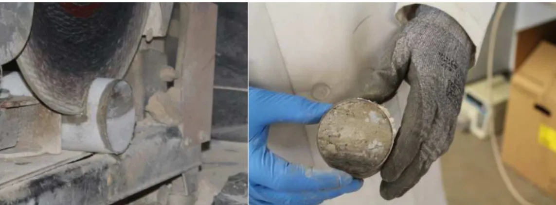
The process of cryogenically collecting 2.5-foot intervals of 2-1/4-inch inner diameter core is summarized in this section. On the left side of Figure 2 there is a cross-section of the cryogenic coring tools. On the right side of Figure 2 there is the diagram with steps 1, 2, and 3 of the cryogenic core collection process. Following Kiaalhosseini et al. (2017), the first step advances the augers and sample barrel to fill the sample liner with 2.5 feet of core. The second step injects liquid nitrogen to freeze the core inside the sample liner. Freezing generally is accomplished in four to six minutes. The third step produces a frozen plug at the bottom of the 2.5 feet interval and extracts the frozen core from the ground. Lastly, the fourth step removes the sample liner with core from the sample barrel. Once the core in the sample liner is removed from the sample barrel, it is placed in a large cooler surrounded by dry ice. The four steps are repeated until the targeted intervals are collected.
2.2.2 Core Processing: Overview of Steps
Core processing follows methods outlined in Sale et al. (2016), Kiaalhosseini et al. (2017), and Olson et al. (2016). Notable relevant advancements to core processing procedures are outlined in this section.
2.2.3 Core Processing: Cutting plan
As a first step, a core cutting plan is advanced based on actual core recovery. Selected intervals for subsampling are based on 1) avoiding the ends of core where samples may be
biased, 2) obtaining subsample over uniform intervals, and 3) addressing conditions at interfaces. Figure 3 provides an example of a cutting plan. The left side of Figure 3 lists 4 cryogenically collected cores at their respective depth interval. The top interval is 24-26.5 feet bgs. Included in Figure 3 is a scale, numbered 0-30 inches, moving right to left from the core’s top. Figure 3 visualizes the collected core with light green for the depth to cut and light brown for the sample ID. Each sample ID has one-inch subsample referred to as “pucks”. The project associated with this cutting plan wanted to increase their sampling resolution, highlighted in yellow, for the third cored interval (29-31.5 feet bgs) because it is in the zone targeted by Laser Induced Fluorescence
Figure 2: Diagrams of Cryogenically collected core Apparatus and Coring Process Kiaalhosseini et al. (2017)
2.2.4 Core Processing: Cutting
Cutting the frozen core has 3 key steps. The first step finds and removes the relevant section of frozen core from a -80 C° freezer. The second step positions an interval of frozen core on a chop saw in a hood. The third step cuts the core as shown in Figure 4. Figure 4 visualizes the saw making a 1-inch cut and a freshly cut core ready to be processed with the plastic liner intact. Sale et al. (2016), Kiaalhosseini et al. (2017), and Olson et al. (2016) outlined the use and definition of 1” frozen core sections as hockey “pucks”. There is a key modification that needs to be addressed. For each sample ID, we now cut two subsequent 1” “pucks” for each sample ID. These are referred to as Puck1 and Puck2. Puck1 is the top sample and is quartered for
biogeochemical analyses (Subsample A), methanol extraction (Subsample B), and future analysis (Subsample D) as outlined in Sale et al. (2016), Kiaalhosseini et al. (2017), and Olson et al. (2016). The entire sample from Puck2 (Subsample C) will be used for visual observation and saturation calculations as outlined in Sale et al. (2016), Kiaalhosseini et al. (2017), and Olson et al. (2016). After Puck1 and Puck2 are cut for a sample ID, any remaining core is cut and archived (Subsample E).
2.2.5 Core Processing: Sample Preservation
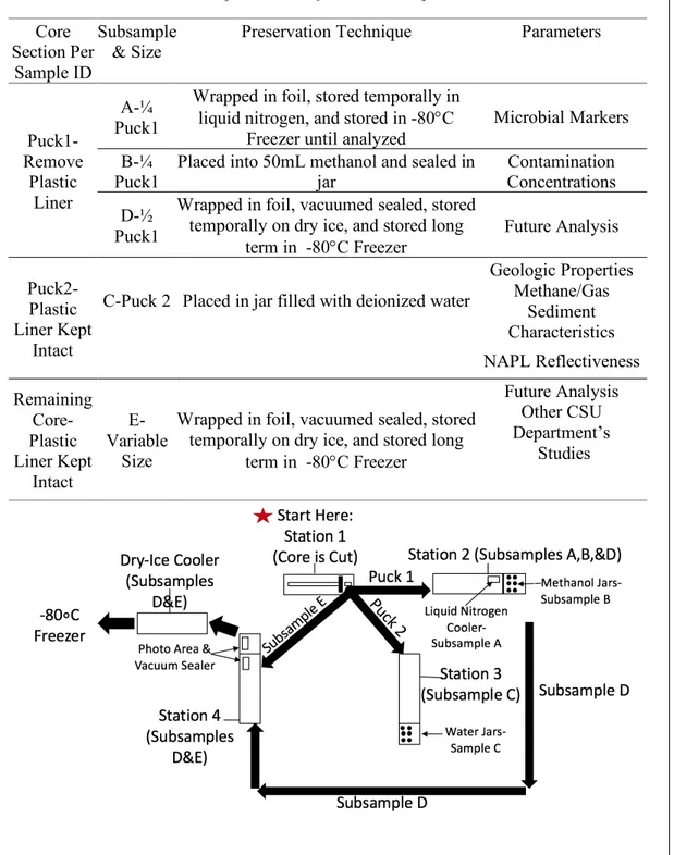
Each Sample ID is guaranteed to have subsamples A, B, C, and D with the possibility of a subsample E. Every subsample’s size, preservation technique, and purpose is summarized in Table 10. During cutting, there are four work stations that each have a set responsibility as visualized in Figure 6. Following Figure 6, Station 1 cuts the core at planned intervals. Station 2 receives, removes plastic liner, and quarters Puck1 into subsamples A, B, and D. Subsample A is wrapped in foil and preserved in liquid nitrogen. Subsample B is preserved in 50 mL of methanol (Figure 5) for microbial and contaminant testing respectively. Any remaining material of Puck 1, subsample D, is sent to station 4 to be vacuum sealed as an archive sample. Station 3 preserves all of Puck2, Subsample C, in a 1-pint Ballä jar for parameters outlined fully in Table 10. Finally, Station 4 vacuum seals remaining core from Puck1, Subsample D, and any
remaining core between sample IDs, Subsample E, for future use (Figure 5). All vacuum sealed core is kept temporally in dry ice coolers before being stored in -80C freezers.
There is a notable, relevant advancement in methods from Sale et al. (2016),
Kiaalhosseini et al. (2017), and Olson et al. (2016) at station 3. Previous methods outlined a quarter of a puck lowered into a ~100ml beaker of water. The results from these methods did not lead to consistently accurate analysis of fluid saturation as the quartered section was loose and did not retain its in-situ physical properties. Currently we take Puck2, with the plastic liner intact, and lower it into a 1 pint Ballä pint jar filled with de-ionized water. Figure 13 shows the type of Ball pint jar used. The weight of the water being displaced by Puck2 is carefully
measured. Using Puck2, as a full 1 inch “puck”, has 3 very positive attributes. The first is greater volumes of soil and water leads to easier weighting procedures. Additionally, the error associated with measuring the displaced water impacts large volumes much less. Finally, the intact plastic casing retains the in-situ pore space, saturations and other physical properties.
Table 10 : Description of subsample size, designation, preservation technique, and parameters for each Sample ID
Core Section Per
Sample ID
Subsample & Size
Preservation Technique Parameters
Puck1-Remove Plastic Liner A-¼ Puck1
Wrapped in foil, stored temporally in liquid nitrogen, and stored in -80°C
Freezer until analyzed
Microbial Markers B-¼
Puck1
Placed into 50mL methanol and sealed in jar
Contamination Concentrations D-½
Puck1
Wrapped in foil, vacuumed sealed, stored temporally on dry ice, and stored long
term in -80°C Freezer Future Analysis Puck2- Plastic Liner Kept Intact
C-Puck 2 Placed in jar filled with deionized water
Geologic Properties Methane/Gas Sediment Characteristics NAPL Reflectiveness Remaining Core-Plastic Liner Kept Intact E- Variable Size
Wrapped in foil, vacuumed sealed, stored temporally on dry ice, and stored long
term in -80°C Freezer
Future Analysis Other CSU Department’s
Studies
Figure 6: General overview of stations and subsamples (A,B,C,D, and E) for each Sample ID
2.3 Sample analysis
The following presents methods including the steps of visual logging, contaminant identification, and microbial identification outlined by Sale et al. (2016), Kiaalhosseini et al. (2017), and Olson et al. (2016).
2.3.1 Visual
The physical properties were evaluated by a Professional Geologist, Dr. Sale, in
accordance with documented process in Sale et al. (2016), Kiaalhosseini et al. (2017), and Olson et al. (2016). Figure 7 shows jars ready to be logged and a jar with NAPL fluorescing under UV light. The properties are presented under USCS classification to reuse previously established graphic choices as outlined in Figure 8. I, Eric Roads, participated in identifying physical
properties for sites since January 2019 in order to effectively evaluate previous reports and data.
2.3.2 COC
COC analysis for chlorinated solvents and hydrocarbons follows methods outlined in Sale et al. (2016), Kiaalhosseini et al. (2017), and Olson et al. (2016). A Gas Chromatography Flame Ionization Detector measures the COCs in the methanol, Subsample B, and water jar, Subsample C, unless specified otherwise. As mentioned in (Sale et al. 2016), (Kiaalhosseini et al. 2017), and (Olson et al. 2016), each contaminant was freshly benchmarked using a known standard for every analysis. Benchmarks from previous projects were compared with new benchmarks for validity verification. The weights of all jars, fluids, samples, and plastic liners are meticulously recorded to solve calculations of porosity, water saturations, gas saturations, and NAPL saturations as outlined in Sale et al. (2016), Olson et al. (2016) and Kiaalhosseini et al. (2017).
2.3.3 Microbial
Microbial analysis for Subsample A, Subsample D, and Subsample E follows the methods outlined in (Sale et al. 2016), (Kiaalhosseini et al. 2017), Irianni-Renno and (Olson et al. 2016). Microbial data is not used in this thesis.
2.4 Data Analysis
The following presents methods for a relational database and primary visualization tool. This section further presents the methods for the analytical steps required to differentiate
between transmissive and low-k zones, calculate mass in place in zones, calculate percentage of total mass in place, and provide intra-site and inter-site comparisons.
2.4.1 Database: Need for gINTä and Use of Excelä
equations and solutions to be quickly and easily applied to large sets of data. The program used to store this data needs to be a relational database. Accessä is a usable relational database based on Excelä. Unfortunately, Accessä does not have any preprogrammed visualization options that would meet our needs. Bentley Academia’sä program gINTä is a relational database using the Accessä architecture. gINTä includes easy-to-use, multifunctional, and highly modifiable capabilities to visualize data-by-depth. Thus, gINTä is used exclusively for any data-by-depth visualization requirements for this thesis. Excelä is still used to visually present mass in place data and statistic plots.
2.4.2 Database: Standardization
The purpose of gINTä for cryogenically collected cores is to assemble all previous, current and future cryogenically collected cores to a single database that provides standardized data-by-depth visuals and allows for multiple cores from differing sites to be compared. The features and complexity of the visuals are developed on a project and purpose basis. This has led to many different visual features and archaic visualization outputs. For this project, there is one type of standardized gINTä forms that will be used. Figure 9 is an example of this gINTä form that outputs available information for a single core on a single sheet. Figure 9 includes a legend that is not included in gINT’sä output features but was added afterwards for descriptive
simplicity. Notable features include a geology section that includes depths from surface (ft), Sample ID #, sediment color, USCS sediment graphics, NAPL visual response, transport designation, and water table depth. The NAPL response is colored with white for missing section, light grey for nothing and darker greys for increasing reflective response. The transport designation is between transmissive (blue) and low-k (black). The remaining gINTä objects are
data-by-depth plots that use standardized, unique colors for each parameter. Due to various circumstances, certain sites do not have complete data sets to output all information and thus will have missing details.
2.4.3 Analytical: Transmissive – Low k
A key objective for this thesis is to resolve the distribution of contaminant mass in transmissive and low-k zones. The methods used to classify the transmissivity of sample are outlined in the following text. Using the visual logs of each Sample IDs, we review each
borehole at a site to resolve transmissive and low-k zones. Conceptually, transmissive and low-k zones are thought to have at least a two order magnitude difference in hydraulic conductivity based on visual observations. If a difference of two orders of magnitude exists, the borehole has both transmissive and low-k zones. Two general conditions are observed in the cores and are presented in this thesis. The first is predominately sandy subsurface media. The first type of site defines the USCS classification silty sand and any particle smaller as low-k and the USCS
classification fine sand and any particle larger as transmissive. The second type is predominately silt/clay subsurface media. The second type of site defines the USCS classification sandy silt and any particle smaller as low-k and the USCS classification silty sand and any particle larger as transmissive. This thesis presents the dividing point between the transmissive and low-k zones based on visual observations as opposed to actual measurements.
26
Each site was characterized based on an analysis of all the boreholes on site to determine a general distribution of subsurface media. In the future, consideration should be given to using cryogenic cores in laboratory studies to directly measure permeability.
2.4.4 Analytical: Total Mass in Place in Borehole, Transmissive Zones, and Low-k Zones This section outlies the mathematical methods and equations used. The mass in place (M/L2) for each Sample ID is defined as
Equation 1: Mass in Place (M/L2)
!"# = !# ∗ &#∗ '(
where !# is the mass of contaminant in mass of soil (M/M), &# is the depth interval represented by the Sample ID (L), and '( is the bulk density (M/L3) of the Sample ID. '(,# is calculated for each Sample ID, unless information is unavailable or incomplete, and is defined as
Equation 2: Bulk Density (M/L3)
'(,# = *# ∗ '+,-./0
where *# is our calculated porosity (L3/L3) and '+,-./0 is the density (M/ L3) of quartz (2.65 gm/cm3). The total mass in place (M/L2) for the borehole is defined as
Equation 3: Total Mass in Place (M/L2)
!"12/-3 = 4 !"# 5
where 8 is the number of Sample IDs in the borehole, !"# is the mass in place (M/L2) for the selected parameters, and the operation sums all sample IDs for a borehole. The total mass in transmissive zones is defined as
Equation 4: Total Mass in Place (M/L2) in Transmissive Zones
!"1 = 4 !"#
59:;<=>?==?@A
#6#B /.-5DE#DD#FG,7
where 81.-5DE#DD#FG is the number of Sample IDs in transmissive zones, “H = HI JKL8MNHMMHOP, 1” is selectively adding mass in transmissive zones only, !"# is the mass in place (M/L2) for the selected parameters, and the operation sums all transmissive sample IDs for a borehole. The total mass in low-k zones is defined as
Equation 5: Total Mass in Place (M/L2) in Low-k Zones
!"RS = 4 !"# 5TUV W
#6#B 32X S,7
where 8R2X S is the number of Sample IDs in low-k zones, “H = HI YZ[ \, 1” is selectively adding mass in low-k zones only, !"# is the mass in place (M/L2) for the selected parameters, and the operation sums all low-k sample IDs for a borehole. The total mass of all contaminants (M/L2) in the borehole is defined as
Equation 6:Total Mass of Contaminants in Place (M/L2)
!"12/-3,]^_`a` = 4 !"12/-3, # 5bU<c;>?<;<c=
Where 8d25/-E#5-5/D is the number of number of contaminants measured in the borehole, H = 1 is adding the total mass of each contaminant, !"12/-3,# is the total mass in place (M/L2) for the selected contaminant, and the operation sums all total contaminant masses for a borehole. Hydrocarbon boreholes sum benzene and TPH. Chlorinated solvent boreholes sum DCE, PCE, TCE, and/or VC.
The amount of core lost from drilling needs to be considered in assumptions in order for the mass in the hole to be continuous. Any lost length of core from the sampling procedure was divided evenly and the top half of lost core copies data from the point before it and the bottom half of lost core copies data from the point after it. This was done instead of ignoring losses or only using a single point because the data points before and after the lost core are usually significantly different.
2.4.5 Analytical: Fraction of Primary COC in Transmissive and Low-k Zones The fraction of sampled borehole that is transmissive (L/L) is defined as
Equation 7: Fraction of Sampled Borehole that is Transmissive (L/L) ef= g/.-5DE#DD#FG/g]-Ei3Gj
where g/.-5DE#DD#FG (L) is the feet of core that is defines as transmissive and g]-Ei3Gj (L) is the total feet of core sampled. The fraction of sampled borehole that is low-k (L/L) is defined as
Equation 8: Fraction of Sampled Borehole that is Low-k (L/L)
where gR2X S (L) is the feet of core that is defines as low-k and g]-Ei3Gj (L) is the total feet of core sampled. The fraction of sampled borehole that is transmissive (L/L) and the fraction of sampled borehole that is low-k (L/L) are defined as
Equation 9: Fractions of Sampled Borehole equal 1 (L/L) ef+ ekl= 1
where the sum of the two variables equals one. In this thesis percentages are the preferred method of data presentation. It is important to transform the mass in place (M/L2) to fraction of mass (M/M) in each zone for each core. It is possible to compare mass in place (M) between sites and cores, but this paper needs to be able to compare cores that have drastically different masses of contamination, different depth intervals and different COCs. The fraction of contaminant of concern, non#, (M/M) in the transmissive zones of the borehole is defined as
Equation 10: The fraction of contaminant of concern, COCi, (M/M) in the transmissive zones of
the borehole
pqpr ef= !"1(non#)/!"12/-3(non#)
Equation 11: The fraction of contaminant of concern, benzene, (M/M) in the transmissive zones of the borehole
pqpuvwxvwv ef = !"1(non(G50G5G)/!"12/-3(non(G50G5G)
where !"1(non#) is the mass of the non# per area (M/L2) in the transmissive zones and !"12/-3(non#) is the total mass of the non# per area (M/L2) in the borehole. The fraction of contaminant of concern, non# (M/M), that is in low-k zones of the borehole is defined as
Equation 12: The fraction of contaminant of concern, COCi, (M/M) in the low-k zones of the
borehole
pqpr ekl = !"RS(non#)/!"12/-3(non#)
Equation 13:The fraction of contaminant of concern, benzene, (M/M) in the low-k zones of the borehole
pqpuvwxvwv ekl = !"RS(non(G50G5G)/!"12/-3(non(G50G5G)
where !"RS(non#) is the mass of the non# per area (M/L2) in the low-k zones and !"12/-3(non#) is the total mass of non# per area (M/L2) in the borehole. The fraction of non
# (M/M), that is in transmissive zones and the fraction of non# (M/M) that is in low-k zones is defined as
Equation 14: The fractions of contaminant of concern equals 1 pqpr ef+ pqpr ekl = 1
where the sum of the two variables equals one. In this thesis percentages are the preferred method of data presentation.
The focus of the statistics is on the difference between the percent of the borehole that is low-k and the percent of contaminant or contaminants in low-k zones (L/L-M/M). This is defined as
Equation 15: Difference between the percent of the borehole that is low-k and the percent of contaminant or contaminants in low-k zones (L/L-M/M)
Where IRS is the fraction of sampled borehole that is low-k (L/L) and non# IRS is the fraction of non# (M/M) that is in low-k zones of the borehole. The difference is then put through a basic statistical analysis and plot as a box plot with extra visuals. All statistics are included in inter-site analysis. Intra-inter-site analysis does not include statistics because only Site A and B would have enough boreholes, seven boreholes, for such analysis.
2.4.6 Analytical: Intra-Site and Inter-Site Comparison
The mass in place and percent mass in place will be used to provide comparisons of cores across a single site and across multiple sites. Every borehole and every site will have both mass in place data and percent of total mass in transmissive and low-k zones. The intra-site analysis will include a graphic and tabular summary of all boreholes and a site average specific to each site. The inter-site analysis will include selective borehole comparisons from differing sites and graphic and tabular summaries of all COCs at hydrocarbon sites, chlorinated solvent sites and all contaminated sites.
CHAPTER 3: RESULTS
This section presents the results for intra-site comparisons and inter-site comparisons. Results presented herein are good to no more than a single significant figure. Additional significant figures are retained to facilitate checking sums and future manipulation of values. The results for inter-site comparisons are presented on a site by site basis. They classify the subsurface media into transmissive or low k zones, outline key features of borehole
concentrations by depth, calculate the mass of contaminants in zones, and calculate the percent of mass of contaminants in zones. The results for inter-site comparisons are presented on a contaminant basis extending across sites. Inter-site results present comparisons for hydrocarbon contaminated boreholes, comparisons for chlorinated solvent contaminated boreholes, and comparisons for all boreholes together. Inter-site results include relevant statistics
accompanying mass in place visuals. As a special note, the principle objective of this work is to demonstrate methods for intra-site and inter-site comparisons of cryogenic core data. An
exhaustive review of the basis for the conditions observed in transmissive and low-k subsurface media is beyond the scope of this thesis.
3.1 Intra-Site Analysis
Analysis begin with intra-site results. Sites A-H are presented in order with their respective boreholes.
3.1.1 Intra-Site A
Site A is a former wood treatment site where PCP was employed in a mineral carrier oil. The geologic setting is a glacial outwash at the terminus of an extinct continental ice sheet. At
Site A, media containing silt and finer media is characterized as low-k. All media without silt is characterized as transmissive.
3.1.1.1 Contamination by Depth
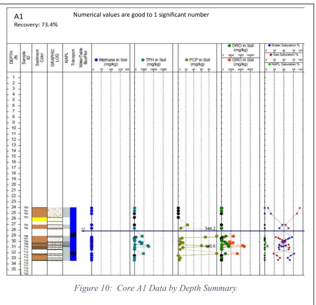
Figure 10 is an illustrative graphic from gINTä that advances cryogenic coring data by including geologic and contaminant data-by depth for the cored interval from Borehole A1. Starting on the left, the geologic graphic includes depth from ground surface, Sample ID, sediment color, graphic log, NAPL visual, transport visual, and 3 points for water table data. The contaminant data-by-depth then plots methane, TPH, PCP, DRO, and GRO concentrations. Finally, this graphic plots the saturations percentages of water, gas, and NAPL. The key findings for borehole A1 include:
• 73% of the core was recovered.
• The zone targeted by LIF is largely characterized by transmissive zones with low-k zones present in areas of high contamination.
• A1 successfully bounds the zone targeted by LIF (26-32 feet bgs) inside the small cored interval (24-33.5 feet bgs).
• A1 has the most mass of contaminant PCP for all the boreholes collected from Site A with several, large off scale concentration spikes.
• There does not appear to be a correlation with concentration spikes of TPH and PCP.
• The percentage of gas increases past 50% below the water table at the depth of highest contamination (31feet bgs). This could be evidence for natural
Borehole A1 has both transmissive and low-k zones and is a good representative of the LNAPL contamination of other boreholes at Site A. However, A1 is an outlier due to the high
concentration of PCP observed. Like the other boreholes on site, the saturations percentages of water, gas, and LNAPL along with the presence of methane provide evidence for active
microbial populations Garg et al (2017).
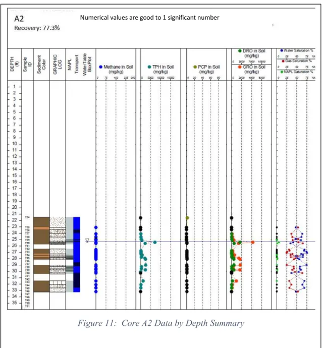
Figure 11 is an illustrative graphic from gINTä that follows the format of Figure 10. The key findings for Borehole A2 include:
Figure 10: Core A1 Data by Depth Summary Numerical values are good to 1 significant number
• The zone targeted by LIF is largely characterized by transmissive zones with definitive low-k pockets throughout the cored interval.
• A2 successfully bounds the zone targeted by LIF (25-31.5 feet bgs) in the cored interval (21.5-33 feet bgs).
• A2 has almost no PCP contamination found. There is a single data point that positively measured PCP (21.5feet bgs).
• The gas percentage below the water table pushes past 50% when the area has high contamination (25.5 feet bgs, 27.5 feet bgs, and 29.5 feet bgs) and 0.5%-5% NAPL saturation percentages. This could be evidence for natural attenuation, Garg et al (2017) Kiaalhosseini et al. (2017).
Borehole A2 has a similar trend for contamination that is seen in boreholes A3-A7. A2 has both transmissive and low-k zones and is a good representative of the LNAPL and PCP contamination of other boreholes at Site A. Like the other boreholes on site, the saturations percentages of water, gas, and LNAPL provide evidence for active microbial populations Garg et al (2017).
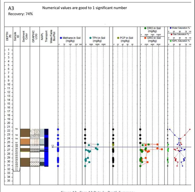
Figure 12 is an illustrative graphic from gINTä that follows the previous format. The key findings for Borehole A3 include:
• 74% of the core was recovered.
• The zone targeted by LIF looks well represented by both transmissive and low-k zones throughout the cored interval.
Figure 11: Core A2 Data by Depth Summary Numerical values are good to 1 significant number
• A3 successfully bounds the zone targeted by LIF (25-31.5 feet bgs) inside the cored interval (21.5-31.5 feet bgs).
• A3 has a small interval (24.5-26 feet bgs) that is PCP contaminated. It is still a magnitude less contamination than A1.
• Both times the gas saturation passes 50% there is a 1-4% NAPL saturation and high TPH concentrations at their respective depths. This could be evidence for pooling of natural source zone depletion (NSZD) gasses as they try to vertically move, Garg et al (2017) Kiaalhosseini et al. (2017).
Borehole A3 continues the trend in contamination that is seen in boreholes A2, and A4-A7. A3 is well represented by both transmissive and low-k zones and is a good representative of the
LNAPL and PCP contamination of other boreholes at Site A. Like the other boreholes on site, the saturations percentages of water, gas, and LNAPL provide evidence for active microbial populations Garg et al (2017)
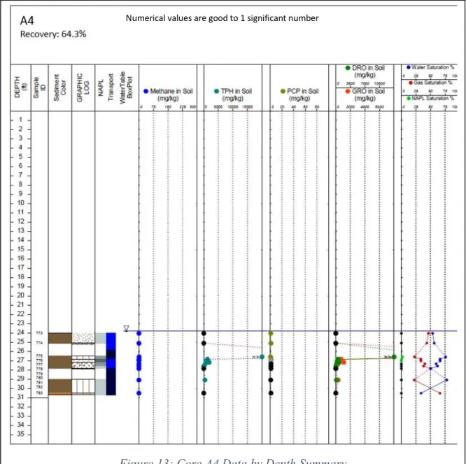
Figure 13 is an illustrative graphic from gINTä that follows the previous format. The key findings for Borehole A4 include:
• 64% of the core was recovered.
• The core is evenly represented by transmissive and low-k zones. Transmissive zones dominate the top half where low-k zones dominate the bottom.
Figure 12: Core A3 Data by Depth Summary