Indoor Positioning at Arlanda Airport

(1)

Indoor Positioning at Arlanda Airport

AHMAD AL RIFAI

(2)

(3)

Indoor Positioning at Arlanda Airport

AHMAD AL RIFAI

Master of Science Thesis performed at the Radio Communication Systems Group, KTH. June 2009

(4)

KTH School of Information and Communications Technology (ICT) Radio Communication Systems (RCS)

TRITA-ICT-EX-2009:75 c

Ahmad Al Rifai, June 2009

(5)

Abstract

Recent years have witnessed remarkable developements in wireless positioning systems to satisfy the need of the market for real-time ser-vices. At Arlanda airport in Stockholm, LFV - department of research and developement wanted to invest in an indoor positioning system to deliver services for customers at the correct time and correct place. In this thesis, three different technologies, WLAN, Bluetooth, and RFID and their combination are investigated for this purpose. Several approaches are considered and two searching algorithms are compared, namely Trilateration and RF fingerprinting. The proposed approaches should rely on an existing WLAN infrastructure which is already de-ployed at the airport. The performances of the different considered solutions in the aforementioned approaches are quantified by means of simulations.

This thesis work has shown that RF fingerprinting provide more accurate results than Trilateration algorithm especially in indoor en-vironments, and that infrastructures with a combination of WLAN and Bluetooth technologies result in lower average error if compared to infrastructures that adopt only WLAN.

(6)

(7)

Acknowledgements

I owe my deepest gratitude to my supervisor at KTH Luca Stabellini for his valuable comments and guidance throughout my work. My great thanks also go to my examiner Ben Slimane who encouraged me for this work and for his comments as well. I can not forget my friends for all the great times we had throughout these years.

I am indebted for all my acheivments so far to my family; my sisters, my father and especially my mother for their endless love, support, and encour-agement.

My thanks go as well to Fritjof Andersson and Christine Hiller at LFV. A heartful thank goes to my fiance Maha who stood by my side all the time. Your ambition has always pushed me forward.

(8)

(9)

List of Tables

1 Different delays for different physical layers . . . 7

2 Power classes . . . 11

3 parameters values . . . 22

4 25, 50 and 90 percentiles for WLAN-only approach . . . 23

5 25, 50 and 90 percentiles for the combined scenario, case 1 . . . . 24

6 25, 50 and 90 percentiles for the combined scenario, case 2 . . . . 25

7 25, 50 and 90 percentiles for the WLAN-only scenario with 6 APs against the combined one with 4 APs and 20 TRXs . . . 26

(12)

List of Figures

1 WLAN network example . . . 5

2 Three different RFID tags. . . 10

3 Different Bluetooth topologies . . . 12

4 Bluetooth signaling procedure . . . 13

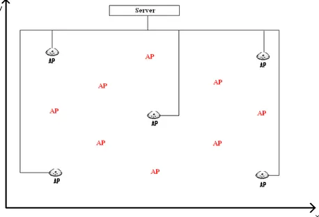
5 Adding WLAN APs to the existing Network . . . 14

6 Adding Bluetooth transceivers to the existing Network . . . . 15

7 Adding WLAN access points and Bluetooth transceivers to the existing Network . . . 16

8 Trilateration method with three control points . . . 17

9 Fingerprinting algorithm: offline and online phases . . . 18

10 Trilateration algorithm: comparison among four different densities of WLAN access points. . . 23

11 Trilateration algorithm: comparison among four different densities of APs and TRXs, case 1 . . . 24

12 Trilateration algorithm: comparison among four different densities of APs and TRXs, case 2 . . . 25

13 WLAN-only (6 APs) against the combined scenario (4 APs , 20 TRXs) using Fingerprinting algorithm. . . 26

(13)

List of Abbreviations

AFH Adaptive Frequency Hopping ACL Asynchronous Connectionless

ADSL Asymmetric Digital Subscriber Line AP Access point

AOA Angle Of Arrival BER Bit Error Rate BT Bluetooth

CCK Complementary Code Keying CRC Cyclic Redunduncy Check

CSMA/CA Carrier Sense Multiple Access with Collision Avoidance DBPSK Differential Binary Phase Shift Keying

DAB Digital Audio Broadcasting

DQPSK Differential Quadrature Phase Shift Keying DSSS Direct-Sequence Spread Spectrum

EPE Ekahau Positioning Engine ERP Extended Rate Physicals

FCC Federal Communications Commission FHSS Frequency-Hopping Spread Spectrum GFSK Gaussian Frequency-Shift Keying GPS Global Positioning System

HF High Frequency

HCI Host Controller Interface

IEEE Institute of Electrical and Electronics Engineers IrDA Infrared Data Association

ISM Industrial, Scientific and Medical LAN Local Area Network

LF Low Frequency LTE Long Term Evolution MU Moving Unit

(14)

PBCC Packet Binary Convolutional Code PER Packet Error Rate

QPSK Quadrature Phase Shift Keying RFID Radio Frequency Identificaion SCO Synchronous Connection-Oriented SIG Special Interest Group

SNR Signal to Noise Ratio TOA Time Of Arrival UHF Ultra High Frequency

WLAN Wireless Local Area Network WSN Wireless Sensor Networks

(15)

1 Introduction

1.1 Background

Mobile communication applications have evolved dramatically in recent years. Shifting from voice and text messaging services to video calling and internet surfing, opened the gate for far more complex applications that have been implemented or are currently being developed. Location based applica-tions such as Global Positioning System (GPS) have also been widely used for positioning and tracking in outdoor environments. However, this technology is not efficient in indoor environments due to high signal attenuation, thus alternative solutions have to be designed.

Several wireless technologies exist now for indoor positioning, namely Blue-tooth, Wireless Local Area Network (WLAN), Wireless Sensor Network (WSN), Infrared Data Association (IrDA), home RF, Radio Frequency Identification (RFID) etc... . Bluetooth is very popular nowadays and most of the new wireless handsets or mobile phones are equiped with a Bluetooth interface. Bluetooth is a short range technology which works in the unlisenced 2.4 GHz Industrial, Scientific, and Medical (ISM) band and is very useful for localization. Using Bluetooth, position estimation could be done either at the mobile unit or in a centralized way by the positioning system that will estimate the position from received data. WLAN is also another short range technology that works in the 2.4 GHz ISM band and the 5 GHz Unlicensed National Information Infrastructure UN-II band. Since WLAN access points are linked together through a higher level system, signals from mobile units could be used to estimate their position. Similar to Bluetooth, localization could also carried out both at the mobile unit as well as the access point. Apart from the mentioned technologies, RFID systems play an important role in localiza-tion applicalocaliza-tions. In this case, a tag is attached to an item, person, or animal and a reader retreives data from these tags on a periodic or demand base. RFID systems work in differnt frequency bands and this affects their range of operation. WSN is a promising technology as well for communications in indoor environments and can be exploited for localization purposes [1]. The latest version of its standard, IEEE 802.15.4 identifies 6 physical layers working in different frequency bands: 900 MHz, 2450 MHz, 3-5 GHz, and 6-10 GHz supporting different data rates. Home RF is another technology that could be used for localization [2]. It Works in the 2.4 GHz band and uses Frequency Hopping Spread Spectrum (FHSS) scheme to support a data rate up to 10 Mbps and range up to 50 meters. However, home RF is no more under development since 2003 and is rarely used due to high competi-tion from WLAN which supports higher data rates and longer ranges. In a similar manner, IrDA [3] is a widely used technology in remote controlling tasks such as in TV sets and earlier versions of laptops in the period 1990 - 2000. However it is not a good candidate for localization tasks since it requires line of sight between the involved devices.

(16)

In this thesis work, I will focus on investigating three of the mentioned tech-nologies; WLAN, RFID, and Bluetooth for localization purposes in indoor en-vironments. In wireless systems, there is no direct metric that can measure the distance of a mobile unit to some access or reference point. Thus, this distance has to be measured indirectly through other parameters. Several works [4, 5, 6, 7, 8, 9] have considered for this purpose the Received Signal Strength (RSS). This metric has a direct relationship with the distance that can be calculated using proper propagation model. Other metrics like Angle Of Arrival (AOA) and Time Of Ar-rival (TOA) have been considered in the literatures, see for instance [10, 11, 12] and [13, 14, 15] respectively. The later matrics have been investigated thoroughly separately or in junction to acheive better performance.

1.2 Related Work

Significant effort has been accomplished to optimize localization systems, and several methods have been used to estimate locations accurately in WLAN, RFID, and Bluetooth networks. For instance, in [5], a detailed propagation model for WLAN has been considered where losses due to refraction and wall penetration have been considered separately. This can potentially result in more accurate es-timation of distance. The authors have also implemented two different algorithms to control the update procedures of the database which holds values of the recent power levels and their relative estimated distances. [9] introduces a new method called location fingerprinting. The idea tailored by this method is to collect a database of signal strength and spatial coordinates for some reference points in the considered environment. Then an opportune algorithm is used to compare the signal strength of a moving unit with those saved in the database allowing to estimate the position of the considered moving terminal. For estimation, the authors considered both a deterministic approach based on Euclidean or Manhat-tan disManhat-tance, as well as a probabilistic one based on Bayesian localization. The probabilistic approach lead to better estimates due to the fact that more statistical information could be exploited. In [16], a hetrogenous localization system com-bining the Ekahau Positioning Engine (EPE), a software solution which utilizes WLAN infsrastructure, and acoustic localization which is supported by a WSN was proposed. The authors used radio and acoustic signals and calculated the difference of their time of arrival to infer the distance between a mobile unit and a fixed point. Trilateration was also used to estimate the position from at least three different sources. Due to the fact that sound travels slower than radio waves, their tests have shown that this hetrogenous system provides better accuracy than using the EPE system alone especially at boundaries such as walls.

[6] presents a modified version of LANDMARC system [17], for indoor local-ization using RFID tags. LANDMARC uses some known located reference tags instead of employing many readers that could increase the application cost. The

(17)

system uses the Euclidean distance in signal strength as a metric to identify the closest reference tags to the target. Then the algorithm uses weighted mean to estimate the location of the target unit among those closest reference points. How-ever, [6] suggests to use only the Euclidean distance for the close reference tags instead of accounting for all the reference tags available in the database. This will reduce complexity and allow for quick estimates.

[4] presents an overview study of Bluetooh technology for indoor positioning. The aim of the work is to develop a Bluetooth service that is not manufacurer-specific. For this purpose, the authors relied on Host Controller Interface (HCI) commands. Trilateration is used to estimate the location, and signal strength is related to distance using a logarithmic model. [8] suggests a combination of signal strength and scene analysis1

to acheive higher accuracy. In this system, the mobile units measure the signal strength from several Bluetooth access points in the envi-ronment and transmit these information to a main server. At the main server, an RSS map of the environment is built, then the server estimates the position using trilateration utilizing the RSS map that has been already built. In [7], the authors used also RSS to estimate distances from power levels, however, they used Least Square Estimate (LSE) in the trilateration algorithm in order to approximate the coordinates of the mobile unit.

1.3 Purpose of the Thesis

Arlanda is the biggest airport in Sweden and is located in the north of Stock-holm. As part of the developement process, a localizaiton system for indoor en-vironments is thought of as a basis that could be used for many applications by different departments. Examples of the services that could exploit the availabitity of location information are:

1. Localization of employees.

2. Localization of moving objects (luggage, vehicles, etc...) within the airport facility.

3. Advertisement services for customers in the airport.

4. Estimation of population density in several sectors of the airport. 5. More reliable security control.

At Arlanda, a WLAN infrastructure is deployed in all airport sections, and is mainly used to allow internet access to customers. This infrastructure was

1

scene analysis is the usage of scene features whch have been previously observed to obtain conclusion about the location of an object.

(18)

thought to be used in localization for security snd control purposes. The system was originally implemented using a Cisco location appliance, but its performance was tremendously weak. Thus, significant modifications and additions are needed to make the system more accurate. Two major issues arise when thinking about these modifications; how much accuracy one can acheive and at whatcost.

1.4 Problem Formulation

The aim of this thesis work is to compare solutions based on three different tech-nologies, namely WLAN, RFID and Bluetooth, and give recommendation about which one, or which combination of them, is best suitable for an indoor location system at Arlanda airport. The decision will be based on the scenario which gives the lower positioning error with a relative low cost. Futher more, the performance of two different localization algorithms, trilateration and RF fingerprinting will be investigated.

The thesis work should answer the question:

• Based on the existing WLAN infrastructure at Arlanda, how could this network be improved to provide better accuracy?

1.5 Thesis outline

The rest of this report is organized in the following order; chapter 2 presents an overview of the technologies involved in this study, while chapter 3 shows the sys-tem model and the proposed approaches. Chapter 4 shows the simulation results, and finally chapter 5 includes the conclusions and future work.

(19)

2 Technologies Involved

In this part, a general overview of the technologies involved is outlined. At first, we discuss the physical and MAC layers of WLAN which is the deployed infstracture. Following that, RFID and Bluetooth are presented.

2.1 Wireless Local Area Network, WLAN

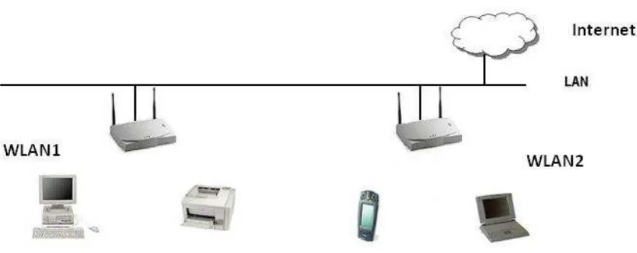
Wireless Local Area Network, WLAN, is a wireless communication system used to replace the existing wired infrastructure at the final link between the end user and the existing wired network. as shown in Figure 1. This technology has been widely used recently in public areas, universities, companies, hospitals, etc... and its benefits are greatly appreciated by the community. The greatest among them are:

Figure 1: WLAN network example

• Cost efficiency by eliminating the costs of bulky wired networks at the final end of the network.

• Mobility where clients are able to roam within the range of the network providing better work efficiency.

• Ease of access to the network where new clients can easily access the network without the need to exist in special locations such as office, meeting rooms, etc...

The evolution of WLAN started in mid 1990s where the first IEEE specification, 802.11, about how WLANs in the 2.4 GHz band should work was released in 1997

(20)

[18]. This version provided a data rate ceiling of 1 or 2 Mbps depending on the used physical layer. Since then, several improvements of this technology have been developed in order to provide higher data rates. 802.11b was released in 1999 to work in the 2.4 GHz and allowing date transfer up to 11 Mbps [19]. In the same period, another standard was also released, namely 802.11a [20], allowing data rate up to 54 Mbps and operating in the 5 GHz band. Despite the high data rate provided, 802.11a faced a major problem of compatibility with older versions of WLANs. In June 2003, 802.11g was released [21]. This version solved the problem of compatibility since it worked in the 2.4 GHz and by making use of the 802.11a OFDM physical layer was able to achieve the same data rate of 54 Mbps. Several other versions were released and many more are still under developement address-ing new problems such as security, spectrum management, region extensions, mesh networking, etc.... A promising standard, 802.11n is expected to be released in De-cember 2009 claiming to support a data rate of up to 300 - 600 Mbps. However, it is important to note that the Wi-Fi Alliance has started to certify products based on IEEE 802.11n Draft 2.0 as of mid-2007.

2.1.1 802.11 Standard Physical Layer

In this section, I will refer only to 802.11b and 802.11g standards. The 802.11b standard encloses a radio spread spectrum technique, namely Direct Sequence Spread Spectrum (DSSS), and one diffuse infrared technique. According to the ETSI regulations, the DSSS technique splits the 2.412-2.472 2

GHz band into 13 22 MHz channels 3

. 3 non-overlapping channels exist in this scenario while adja-cent channels overlap with 5 MHz band difference between 2 consecutive adja-center frequencies. To supply high data rates, 802.11b defines a new coding algorithm, Complementary Code Keying CCK, to support 5.5 and 11 Mbps respectively with the use of Quadrature Phase Shift Keying (QPSK). Binary Phase Shift Keying is used for low data rates. In addition, Dynamic Rate Shifting is used to adapt the data rate to the channel conditions and position of the client in the network. High data rates are used for nearby clients, however for far clients, the system choose low data rates with proper coding and modulation.

The 802.11g physical layer encloses four different physical sublayers;

ERP-OFDM supports data rate up to 54 Mbps. All devices that are identified to have this option will use this physical layer to enhance performance unless an obligation exists to switch to another physical layer.

2

these are the limiting center frequencies according to this regulation.

3

In USA, France, Spain, and Japan, different regulations apply. In USA, 11 channels (2.412-2.462 GHz). In Japan, 14 channels (2.412-2.484 GHz). In France, 4 channels (2.457-2.472 GHz). In Spain, 2 channels (2.457-2.462 GHz).

(21)

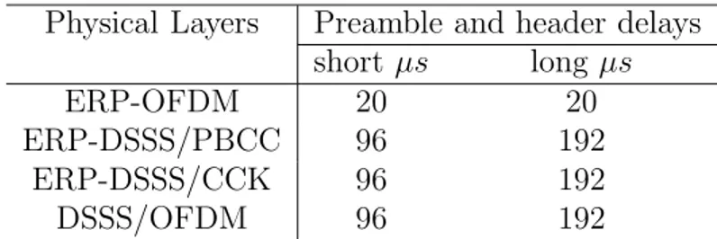
Physical Layers Preamble and header delays short µs long µs ERP-OFDM 20 20 ERP-DSSS/PBCC 96 192 ERP-DSSS/CCK 96 192 DSSS/OFDM 96 192

Table 1: Different delays for different physical layers

ERP-DSSS/PBCC is an updated version of DSSS in 802.11b to support data rates up to 22 and 33 Mbps. The enhancement is due to a better coding algorithm PBCC,Packet Binary Convolutional Code, which was approved as an alternative to CCK.

ERP-DSSS/CCK is the same standard used by 802.11b. It was introduced to support compatibility.

DSSS/OFDM is a hybrid physical layer which was introduced to support inter-operability, where the physical header is transmitted using DSSS where the payload is transmitted using OFDM, Orthogonal Frequency Division Mul-tiplexing. The reason for this is to make sure that even devices which don’t work with OFDM system will still be able to sense the channel correctly since CSMA/CA protocol is used.

OFDM is the enhancement in the physical layer that 802.11g has accomplished over 802.11b. It aims to transmit several signals on one single link or path by com-bining different carriers that operate on different frequencies. These frequencies should be orthogonal so that a receiver which is tuned to a specific frequency will only detect the message that is transmitted on this frequency. Thus, a key feature to assure this accuracy in detection is to have orthogonal carriers which inclusively prevent interference from neighboring frequencies in a tight band.

802.11g obligates communication to be done through short preamble4

rather than long preamble since it reduces packet overhead in the network. This option has been also introduced in the 802.11b standard but as an option for devices which support it. Table 1 shows different delays for different physical layers for short and long preambles as identified in the 802.11g standard.

MAC Layer

The MAC layer is responsible to associate clients with the access points. Usually the client has the ability to choose among existing Access Points (APs) according

4

header holds packet information related to thet physical layer, while preamble is used for synchronization

(22)

to their power level. Once the client is accepted to the join one specific network, he will start communicating on the specified channel of this network (22 MHz wide). If the client is open to several networks, then he will be able to reassoci-ate to another network if he out bounds his own network or due to high traffic on his network. This procedure is usually termed as load balancing. As men-tioned earlier, the 2.4 GHz band is split into 14 overlapping channels where each network will use one channel to communicate through. Thus, applying ”channel reuse” pattern as in cellular networks among neighboring APs will increase system throughput by decreasing the amount of interference. The 802.11b standard also controls how clients will share the network by using the Carrier Sense Multiple Access with Collision Avoidance (CSMA/CA) protocol. CSMA/CA protocol al-lows clients within a network to use the channel without interfering each other; for instance, a client listens first to the link to make sure it is free then waits a random period of time and after that transmits if the channel is still free. The receiver will have to respond back by an acknowledgment ACK to identify the successful reception of the packet. The need of this acknowledgment is because clients can not detect if a collision had happened during the transmission since data is sent via air. The sender will retransmit a packet if an ACK is not received, which means that extra overhead is assumed to exist in the air due to the missed ACK from the recipient side. In addition to the ACK mechanism, 802.11b implements also a Cyclic Redundancy Check (CRC) to compare received data with the supposed sent one. Another feature is the Packet Fragmentation where long packets are split into smaller packets to ensure them to get received since long packets are often more risk to get distorted while in the air.

2.2 RFID

2.2.1 Introduction

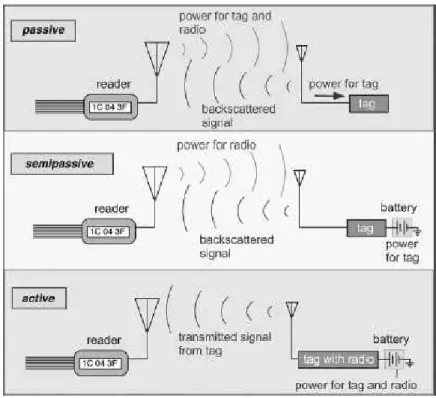
Radio Frequency Identification corresponds to an identification technology which uses radio waves to identify objects or items. The idea of using radio waves for identification goes back to the 50s of the last century, but it took till the 90s to start using this technology after it became possible to manufacture feasible size RFID electronics. An RFID system consists mainly of a reader and a tag. The basic concept is that a reader transmits a radio wave which in turn induces current into the circuit which is printed or installed on the tag. The tag use this current in order to transmit the information that is stored on its internal memory. The amount of information on the tag and its communication range depend mainly on the type of the tag. In particular, three types of RFID tags exist; passive, semi-passive, and active. These are shown in Figure 2.

• Passive tags: this type of tags has no power source. It depends mainly on the received RF waves to extract the power needed to operate its embedded

(23)

circuit using the DC component of the received signal. In addition to that, this tag has no transmitter as conventionaly understood for a device to be able to transmit electromagnetic waves through the air. It works as follows: the reader sends RF carrier in the surrounding environment. A tag which exists in the RF coverage of the reader and has received sufficient energy, powers up its circuit and start to modulate the recieved signal by shunting its coil through a transistor according to the data stored in the memory array of the tag. This modulation of the amplitude of the carrier is detected by the reader which then decode the information according to the coding algorithm used.

• Semi-passive tags: this tag is used when more information than those col-lected by a passive tag need to be stored. These tags use internal batteries to power up the circuit. They still use the backscattered modulation of the received signal to send their information to the reader. These tags are more expensive than passive tags.

• Active tags similar to semi-passive tags, active tags use batteries to power up their circuitry, however, they also use this power while transmitting their information. Active tags are equipped with tranceiver to cover larger areas. Costs increase dramatically if compared to passive tags.

2.2.2 Frequency bands and coverage

RFID systems work in different frequency bands. The most commonly used are the 125/134 kHz (LF band), 13.56 MHz (HF band), 860-960 MHz (UHF band), and the 2.4-2.45 GHz,(microwave band), due their unlicensed nature. The LF and HF systems use inductive coupling while UHF and microwave systems use radia-tive coupling. Inducradia-tive coupling is used in systems where close identification is needed since coupling falls severely as the distance between the reader and the tag increases. On the other hand, radiative coupling is used in systems where wider coverage is needed, but taking into consideration more complex propagation envi-ronments where interference increases remarkably than that in LF and HF systems. Another issue to consider is the range of the RFID system. This metric depends mainly on the power supply and frequency used. Passive tags are mainly used for small range communications in the vicinity of centimeters or 1-2 meter range. However, lately some companies managed to produce some passive tags that can communicate up to 10 or 12 meters. Semi-passive and active tags are intended for wider area coverage. Active tags can operate in the vicinity of 100 meters depending on the environment.

(24)

Figure 2: Three different RFID tags.

2.3 Bluetooth

The idea of naming the current Bluetooth wireless technology by its name refers back to a Viking monarch called Heraled Bluetooth who lived in the 10th century,and was able to unify Denmark and Norway under the same authority. More than that, according to a myth in [22], a monolith was digged out recently and showed a self-portrait of Herald Bluetooth holding a cell phone and a laptop with an antenna. It indicates his forsight though the portrait goes back thousand years ago.

Away from the name, Ericcson was the first to look for a standard that can replace the bulky wiring for devices’ connection. Then in 1998, the Bluetooth SIG was formed to issue the first standard that could be used world wide. This group consists of five pioneer companies in computer and communications technology; namely Ericsson, Nokia, Toshiba, IBM and Intel. Later on, several updates of the standards have been issued promising more advanced technology and better system performance.

(25)

Power Class Maximum Output Power

Minimal Output

Power Power Control

Range 1 100mW (20 dBm) 1mW (0dBm) Pmin < +4dBm

to Pmax

100m 2 2.5mW (4dBm) 0.25mW (-6dBm) Optional:

PmintoPmax

20m 3 1mW (0dBm) N/A Optional:

PmintoPmax

10m Table 2: Power classes

2.3.1 Bluetooth Standard - Physical Layer

Bluetooth is another type of short range wireless technology which operates in the 2.4 GHz free licensed ISM band. This band became free licensed in almost all countries due to the invention of microwave ovens in earlier years. In order for bluetooth devices to operate, the standard divides the 2.4 GHz band into 79 1 MHz channels. The band starts at 2401.5 and ends at 2481.5 GHz. The standard identifies Frequency Hopping Spread Spectrum (FHSS) scheme to trasnmit infor-mation among devices using a pseudo random frequency sequence. Three power classes exist for this standard which are illustrated in table 2. This table has been taken from the IEEE 802.15.1 standard [23].

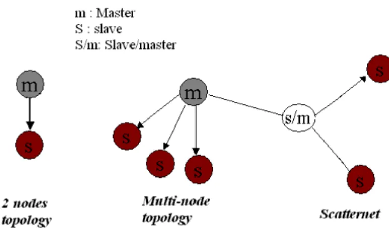
The standard also specifies GFSK as the modulation scheme with a bandwidth time of 0.5, where a binary 1 is represented with a postitive frequency deviation while a binary 0 is represented by a negative deviation. The data transmission rate has a symbol rate of 1 Msymbol/sec. In principle, the standard identifies master and slave or slaves mechanism for devices to communicate in a two-node or multi-node topologies respectively. In a multi-node network, up to 8 slaves could be connected to the same master, where multi-node networks could be connected together to form a bigger network called scatternet. However, slaves within a scatternet could only communicate through their masters. Figure 3 shows the three different types.

A pseudo random frequency sequence is generated by the master according to its physical address and clock. This sequence is communicated to the slave devices in the piconet. A device could be a master or a slave, which depends basically on who will start to establish the connection. However, a master and a slave can exchange roles during operation. A slave responds to the master in the next slot he receives on only if he is addressed by that particular packet, which is how the Bluetooth devices transmit data over air. A simple representation of Bluetooth signaling procedure is shown in Figure 4.

A packet is subdivided into three different blocks; namelyaccess code,header, and payload.

(26)

Figure 3: Different Bluetooth topologies

packet acknowledgment.

• The header contains channel and link control information.

• The payload is intended for information to be sent and some security bits. A packet may be of different lengths; 1, 3 or 5 time slots, where a time slot is 625 µs. Packets are also of different types depending on what kind of data is tranmitted; data, voice, or video.

2.3.2 Bluetooth Standard - The Link Manager

The link manager is responsible for establishing and managing the link. The type of link to be used depends on the type of information that the user wants to send or recieve. Two types of links exist in the Bluetooth standard; SCO and

ACL.

SCO is a symmetric channel between the master and the slave used mainly for audio streaming. On this link, a packet may use 3 or 5 time slots, and is not allowed to be retransmitted. The master can establish an SCO link by a request to the slave with the appropriate parameters. On the other side, the slave can ask for an SCO link by a request to the master, then the master sends back a relevant request with the appropriate parameters.

An ACL link is an assymetric channel that is used for sending data. Only addressed slaves can reply back in the next slot they receive on. There are 3 different packet sizes for the ACL link; 1, 2, or 3 time slots. The master decides which size to use. A slave can ask to change the size of the packet, but that has to be approved by the master to avoid using long packets on noisy channels where BER is significant.

(27)

(28)

3 System Model

As mentioned earlier, several technologies can take up the role to provide the system with the needed information about power levels, distances, and locations. But in this thesis work, the focus will be on WLAN, RFID, and Bluetooth due to their wide usage; WLAN and Bluetooth radio interfaces are included in almost all static and portable devices, and RFID tags are easy to configure and implement in a system and presents a relativly low cost.

In order to reuse the existing infrastructure for localization purposes, some alter-native that might potentially improve the accuracy of localization will be described.

3.1 Approaches

3.1.1 Adding WLAN APs

For this option, a number of APs will be added to reduce the areas where a very weak or no signal is detected. These additional APs will enhance accuracy by providing higher signal strength levels since the physical distance between any arbitrary mobile unit and its surrounding APs will be reduced. More than that, some areas lack the existence of at least 3 APs: these are needed by the trilateration algorithm to work properly, and the additional APs will compensate for this lack as well. In Figure 5, the red marked APs indicates the location of some APs that are thought to be added to the existing network.

(29)

3.1.2 Introduce RFID-WLAN tags

To address some of the services mentioned in section 1.3, items such as luggage trailers and wheel chairs need to be equiped with a device that can be used to identify their identity. RFID tags are mostly used for such tasks, where tags are attahed to the items and a reader monitors their presence in its coverage area. RFID-WLAN tags have also been recently commercialized. These do not require a reader and can use the WLAN infrastructure to transmit their data.

3.1.3 Introducing Bluetooth transceivers

Bluetooth could be merged with the existing WLAN system by adding Blue-tooth transceivers in the gaps where weak signal strength levels from WLAN APs are recorded. They could also be used to complement the set of 3 APs that are required for trilateration in areas where only two APs exist. Notice in Figure 6 that the number of Bluetooth transceivers (bluetooth logo) that are needed ex-ceeds the number of APs needed in theAdding WLAN APs scenario. This is due to the fact even though the transceivers could be of class 1 and may reach up to 100 meters in ideal conditions, many mobile devices uses bluetooth radio interface of class 3 and allow communication ranges of 10 meters only.

(30)

3.1.4 Combining Bluetooth, RFID-WLAN tags, and WLAN

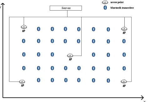
Combining a WLAN infrastracture with Bluetooth access points or base sta-tions to fill the gaps in coverage, and RFID tags to identify particular items, into a single platform and using all the data from these sources would help to increase the accuracy of estimations. Figure 7 sketch the structure of a general system exploiting this solution.

Figure 7: Adding WLAN access points and Bluetooth transceivers to the existing Network

3.2 Searching Algorithms

3.2.1 Trilateration

In radio communication networks, Trilateration is one method used for lo-calization [24]. In principle, a signal should be collected at/from three different control points, base stations or access points, depending whether a centralized or distributed system is deployed. If the signal is detected by more than one control point, then a coverage circle is drawn around each of the control points with a radius proportional to the parameter’s value; signal strength or time of arrival of signal, and the intersection points among the different circles drawn be-come the possible locations of the transmitter. However, having a third control point increases the accuracy by filtering out the incorrect possibility. In case, the

(31)

third circle doesn’t coincide with any of the intersection points, then an averaging method is used to estimate the final position. In wireless networks, this is often the case where the variation in the channel response for each control point doesn’t guarantee precise distance calculation, in addition to the fact that it is hard to have more than three or four control points to detect the same transmitter. Figure 8 shows the principle exploited by this method.

Figure 8: Trilateration method with three control points

In this thesis work, the signal strength is used as a parameter to calculate the relative distance between the control point and the transmitting device, and the average of the closest intersection points as the final position.

3.2.2 RF fingerprinting

Fingerprinting is another method for localization which can be implemented in a centralized or distributed manner. This method can be divided in an offline and an online phase [24]. In the offline phase, data are collected at many predefined reference points in order to form a database. This database includes parameters that identify the considered reference points such as their position, the average signal strength, angle of arrival, and time of arrival of signal or other parameters that could be important for localization purposes. This might represent a very demanding procedure because it requires the manual collection of the aforemen-tioned data at each of the reference points.We further remark that in order to obtain accurate estimates, those data might have to be collected several times in order to obtain average quantities. For the online phase, the system will try to locate an arbitrary transmitter by first measuring some of the available parameters

(32)

(SS, AOA, TOA) and then matching those parameters with the one available in its database, selecting the reference point that corresponds to the best parameter match. Weighted mean, see equation 1, gives better results than arithmetic mean [9], but other averaging methods such as the smallest polygon [25] could also be used to estimate the final position. The weight is found as the inverse of the dif-ference in signal strength between a redif-ference point and the transmitting device for the same AP as shown in equation (2). Figure 9 presents an example of a centralized fingerprinting algorithm where SS and AOA are used as parameters.

a= N X i=1 wiai N X i=1 wi (1) w= 1 |SSref p− SStr| (2)

Figure 9: Fingerprinting algorithm: offline and online phases

3.3 Propagation Model

To obtain system performance that could be considered reliable, one has to model the system as close as possible to reality. In context aware systems, ac-curacy of the system is the first priority. Under this consideration, any type of

(33)

wireless technology could provide signal strength levels based on the deployed in-frastructure. However, the localization algorithm is the key feature which results in the best estimations. Algorithms which depend on RSS to estimate distances to mobile units, should rely on a powerful propagation model that takes into consideration all the factors that causes signal attenuation. According to [26], propagation mechansims include Reflection, Diffraction, and Scattering. • Reflection is the action of a wave striking a large sized object as

com-pared to its wavelength.

• Diffraction is the action of a wave hitting a sureface with irregularities, like the top of a mountain or the corner of a building. The result will be the creation of new secondary waves behind and around the obstacle. • Scattering is the action of a wave striking against objects that are small

if compared to its wavelength. Scattered waves are created which will affect the original wave at the receiver.

Due to its complexity, several propagation models have been proposed by different authors. In the nect section, a brief introduction about wave prop-agation is provided, the propprop-agation models that best work for indoor envi-ronments will also be outlined.

3.3.1 Free space Propagation

In principle, the free space propagation model describes the power den-sity at the receiver due to a line-of-sight path between the transmitter and the reciever, where no obstacles are assumed to affect the signal. Assuming isotropic radiation, equation (3) explains that the power density at the re-ceiver will be equal to the transmitted power uniformly distributed on the surface of the sphere caused by the isotropic radiation. The power at the re-ceiver is just the same power density multiplied with the area of the rere-ceiver antenna as shown in equation (4).

=r = Pt 4πr2 W/m 2 (3) Pr = =rAe = PtAe 4πr2 W (4)

Pt is the transmitted power

Pr is the received power

=r is the power density at the receiver

(34)

r is the distance from the transmitter

These equations are just rough approximations that are mostly used for very long distance communications such as satellites and space detections. The earth is full of elements that can deteriorate waves. Human beings, animals, geographical irregularities, trees, buildings, etc..., are just few ex-amples. As we shrink the environment, these factors become more and more threatening and should not be ignored in calculations. Indoor environments consist of many objects that are static and others that change dynamically. In an office, a desk, board, computer desktop, flowers, etc... are some exam-ples of static objects, whereas people, moving chairs, small instruments are other examples which are dynamically changing. This shows that the chan-nel response will change severely randomly. In the following section, some comprehensive models are presented.

3.3.2 Indoor Models

In this section, the terminology path loss will be refered to as the ratio between the transmitted power and the received power, as illustrated in equation (5).

L = Pt Pr

(5) Some environments require different propagation models according to their structure. As mentioned earlier, objects within these environments change location dynamically which inturn changes the channel response ac-cordingly. From these models we mention the Keenan-Motley model which takes into consideratiion these effects.

However, in this thesis work, the Multi-Wall-and-Floor [27] is used. This model takes into consideration the nonlinear relationship between the cumu-lative penetration loss and the number of penetrated floors and walls which is an affecting factor in determining the power loss. In other words, the pen-etration loss will decrease with the increase number of penetrated walls and floors which are of the same type. Equation (6) shows this relation

LM W F = Lo+ 10nlog(d) + I X i=1 K X k=1 Lwik + J X j=1 M X m=1 Lf jm (6)

where L0 is the reference path loss at 1m, n is the path-loss exponent, d

is the distance from the transmitter to the receiver, Lwik is the attenuation

(35)

explanation as Lwik but for floors, I and J are the number of wall and floor

types respectively, and K and M are the number of penetrated walls and floors of the same type respectively.

3.4 Methodological Approach

The thesis work is based on computer simulations for the different ap-proaches. For this purpose, a Matlab code is written, where the simulations consist of 1000 snapshots for each case of the different approaches. This num-ber of snapshots is sufficient to provide a clear idea about the percentage of error for all the considered cases. After defining the network characteristics, a snapshot consists of randomly placement of a transmitting device within the considered area, path loss and power calculations, applying the searching algorithm, and finally estimation of the position. Error calculation is based on Euclidean distance in two dimensional space between two points. For instance, if (x, y) are the coordinates of the real position, and if (xo, yo) is the system’s estimation, then the error is found to be:

error =p(x − xo)2

+ (y − yo)2

(36)

4 Simulation Results

This part shows the results of the simulations for the considered ap-proaches. Simulations are based on two Matlab codes that respectively em-ulate the Trilateration and Fingerprinting algorithms: both took into con-sideration having one or two technologies involved. Before presenting the obtained results, in the next section some parameters and values which have been used will be defined.

4.1 Parameters’ Definition

For both algorithms, the same sample hall with dimensions (200∗200 m2

) which is very close to the dimensions of all the halls at Arlanda airport has been considered. Also, the control points (WLAN APs and Bluetooth TRXs) are distributed symmetrically over the whole area to acheive maximum possi-ble coverage for a specific number of control points. The propagation model used in these simulations is the MWF model, see equation (6); this takes into consideration different types of walls and floors. The parameters’ values used in this model are summarized in Table5

3.

Parameter Value

WLAN 802.11b trans. power 20 dBm (100 mW) Bluetooth 802.15.1 trans. power 4 dBm (2.5 mW)

Center frequency 2.45 GHz distance path loss 2

Lw 3, 5 dB

Lf 18 dB

Table 3: parameters values

4.2 Trilateration Results

The results of the trilateration simulations show that the number of con-trol points and their distribution over the grid is the main factor that allows to reduce the error. It will be shown that overlapping coverage areas of ad-jacent APs is important for this algorithm to work properly. In the following results, the error in distance, see equation (7), is plotted and discussed.

5

(37)

In Figure 10, the error in distance is plotted for 4 different densities where only WLAN APs exist as control points. The plots show that as the number of APs increase, the error will decrease accordingly. The blue and the green plots correspond to densities of 6 and 13 WLAN APs distributed over the sample hall, 200*200 m2

. The improvement with 13 APs is not significant because there are still uncovered gaps and transmitters that couldn’t be detected by several APs. However with 17 APs, we notice better reduction in the error reaching up,at 50 percentile level, to 10 meters, and to 17 meters with 25 APs. In Table 4 the 25, 50 and 90 percentiles are listed for each density. 0 5 10 15 20 25 30 35 40 0 0.1 0.2 0.3 0.4 0.5 0.6 0.7 0.8 0.9 1 Error (m) Cumulative probability WLAN: 6 WLAN: 13 WLAN: 17 WLAN: 25

Figure 10: Trilateration algorithm: comparison among four different densities of WLAN access points

WLAN density 25% 50% 90% 6 WLAN APs 18.9 27 36.2 13 WLAN APs 16.5 24.8 35.1 17 WLAN APs 8.6 15.1 33.3 25 WLAN APs 5.03 8.6 15.3

Table 4: 25, 50 and 90 percentiles for WLAN-only approach

The second approach is to combine WLAN APs and Bluetooth TRXs in the same grid. For this approach, an equivalent density of APs and TRXs are

(38)

deployed instead of having only APs. Many combinations could be deployed, however, only two cases are considered in this part. The first is shown in Figure 11 with four different densities which are equivalent to the densities shown in Figure 10. For all densities, the number of APs is limited to 4 while the number of TRXs is increased accordingly as the density increase. Table 5 shows the improvements that we can acheive if this case is deployed. The second case is to increase the number of APs and TRXs, Figure 12, where the number of APs is increased till 9 while that of TRXs is increased accordingly. The plots in this figure and values in Table 6 shows that this case has less accurate results than the first one, but still confirm that the combination approach is better than using WLAN APs only.

0 5 10 15 20 25 30 35 40 0 0.1 0.2 0.3 0.4 0.5 0.6 0.7 0.8 0.9 1 Error (m) Cumulative probability WLAN APs: 4, BT TRXs: 90 WLAN APs: 4, BT TRXs: 130 WLAN APs: 4, BT TRXs: 210 WLAN APs: 4, BT TRXs: 20

Figure 11: Trilateration algorithm: comparison among four different densities of APs and TRXs, case 1

density 25% 50% 90% 4 WLAN APs, 20 BT TRXs 7.9 20.6 35 4 WLAN APs, 90 BT TRXs 4.26 6.5 26.2 4 WLAN APs, 130 BT TRXs 3.96 6.09 13.6 4 WLAN APs, 210 BT TRXs 2.49 4.24 8.24

(39)

0 5 10 15 20 25 30 35 40 0 0.1 0.2 0.3 0.4 0.5 0.6 0.7 0.8 0.9 1 Error (m) Cumulative probability WLAN APs: 9, BT TRXs: 40 WLAN APs: 9, BT TRXs: 80 WLAN APs: 9, BT TRXs: 160 WLAN APs: 4, BT TRXs: 20

Figure 12: Trilateration algorithm: comparison among four different densities of APs and TRXs, case 2

density 25% 50% 90% 4 WLAN APs, 20 BT TRXs 7.9 20.6 35 9 WLAN APs, 40 BT TRXs 6.9 16.6 33.8 9 WLAN APs, 80 BT TRXs 4.8 7.7 30.9 9 WLAN APs, 160 BT TRXs 3.3 5.4 10.66

Table 6: 25, 50 and 90 percentiles for the combined scenario, case 2

4.3 Fingerprinting Results

Similar approaches are considered here as those in the Trilateration sim-ulations, where cases with WLAN APs only are compared against scenarios with a combination of WLAN APs and Bluetooth TRXs. The difference here is the efect of the number of reference points on the results as mentioned in section 3.2.2.

In Figure 13, we start by the smallest density of 6 WLAN APs and its equivalent of 4 APs and 20 TRXs combined on the same grid. At first, the number of reference points is set to 63, i.e. on the same area of 200*200 m2

a ref. pt. is collected every 650 m2

. The distribution of these points is fairly symmetrical over the whole area. Then we increase this number to 170 and

(40)

6 APs only 4 APs, 20 TRXs Ref. pts. density 25% 50% 90% 25% 50% 90%

63 7.2 11.3 18.2 5.8 9.1 17.8 170 3.4 5.6 11.3 3.3 5.2 10 325 2.8 4.7 8.8 2.6 3.9 7.6 out coverage conf. int. (95%) 235 ± 5.962 375.8 ± 6.8202 Table 7: 25, 50 and 90 percentiles for the WLAN-only scenario with 6 APs against the combined one with 4 APs and 20 TRXs

325 which is equivalent to a ref. pt. every 235 and 123 m2

. We see from this figure that the performance of the combined scenario is always slightly better than the other. Table 7 shows the error in meters at the 25, 50 and 95 percentile levels for both scenarios and the average of out coveraged with a 95% confidence interval. 0 5 10 15 20 25 30 0 0.1 0.2 0.3 0.4 0.5 0.6 0.7 0.8 0.9 1 Error (m) Cumulative probability

WLAN APs: 6, Ref pts: 63 WLAN APs: 6, Ref pts: 170 WLAN APs: 6, Ref pts: 325

WLAN APs: 4, BT TRXs: 20, ref pts: 63 WLAN APs: 4, BT TRXs: 20, ref pts: 170 WLAN APs: 4, BT TRXs: 20, ref pts: 325

Figure 13: WLAN-only (6 APs) against the combined scenario (4 APs , 20 TRXs) using Fingerprinting algorithm.

Same conclusions can be drawn from Figures 14 and 15 and their corre-sponding Tables 8 and 9 respectively. However, the out of coverage changes drastically due to the fact that more areas are covered. We can see that having only WLAN APs will cover more areas than the combined network, while counting for accuracy, the combined scenario has showed slightly better

(41)

results than the WLAN-only one for all densities of reference points. 0 5 10 15 20 25 30 35 0 0.1 0.2 0.3 0.4 0.5 0.6 0.7 0.8 0.9 1 Error (m) Cumulative probability

WLAN APs: 9, ref pts: 63 WLAN APs: 9, ref pts: 170 WLAN APs: 9, ref pts: 325

63 6.37 10.35 17.15 5.8 8.8 15.45 170 3.8 6 11.25 2.86 4.7 8.7 325 3.2 5 9.1 1.95 3.3 7.8 out coverage conf. int. (95%) 22.2 ± 1.9424 49.5 ± 2.1067 Table 8: 25, 50 and 90 percentiles for the WLAN-only scenario with 9 APs against the combined one with 6 APs and 30 TRXs

(42)

0 5 10 15 20 25 30 35 0 0.1 0.2 0.3 0.4 0.5 0.6 0.7 0.8 0.9 1 Error (m) Cumulative probability

WLAN APs: 15, ref pts: 63 WLAN APs: 15, ref pts: 170 WLAN APs: 15, ref pts: 325

63 5.4 8.9 16.8 4.75 7.9 15.35 170 2.75 4.4 9.39 2.25 3.5 7.8 325 2.25 3.5 6.6 1.5 2.46 6.2 out coverage conf. int. (95%) 3.2 ± 0.8979 4.4 ± 0.929 Table 9: 25, 50 and 90 percentiles for the WLAN-only scenario with 15 APs against the combined one with 9 APs and 52 TRXs

(43)

5 Conclusion and Future Work

5.1 Conclusion

In this thesis work, WLAN, Bluetooth, and RFID technologies have been evaluated to give recommendation to the department of development and research at LFV, Arlanda airport, about which technology or a possible com-bination of them could serve best for positioning services. In addition, two localization algorithms, namely Trilateration and RF fingerprinting, have been tested to find the one that give higher accuracy.

A WLAN network already exists at Arlanda to provide internet services for customer, so based on the existing infrastructure, the work has proposed three different approaches. The first one is to add more WLAN APs in areas where the coverage is poor or doesn’t exist. The second is to add Bluetooth TRXs in these areas and combine them with the WLAN APs into one cen-tralized system that can extract their information and draw results. The third proposal is to add Bluetooth TRXs and RFID tags following the same procedures as in the second proposal. It has been shown that according to the specifications of the company’s needs that RFID tags will only increase the scope of the services since the company is interested to deploy WLAN-RFID tags to eliminate the need for WLAN-RFID readers. Thus, WLAN-RFID was not included in the simulations. The first two proposals have been tested using both Trilateration and RF fingerprinting algorithms.

For the Trilateration algorithm, the simulations have shown that a net-work of WLAN APs and Bluetooth TRXs has always better performance in reducing the error between the position of a transmitting device and the system estimation than having a WLAN-only network. More than that, the results have also shown that increasing only the number of Bluetooth TRXs while keeping the number of WLAN APs fixed to its origin will serve better than increasing both of them.

On the other side, the results of using RF fingerprinting algorithm indi-cate similar behaviour with the following exceptions; Acheiving better cover-age depends mainly on the number of APs and/or TRXs and the combination of them. More than that, deploying only WLAN APs maintains higher cov-erage than deploying a combination of WLAN APs and Bluetooth TRXs for lower densities. However, increasing the accuracy of the system is done through increasing the number of reference points. Following this, deploying a combined network of APs and TRXs has shown always slightly better

(44)

per-formance than deploying WLAN-only network.

5.2 Future Work

In this thesis work, the main interest was to reduce the error in distance between the position of a transmitting device and the system’s estimation. This constitutes a major factor in evaluating the performance of localization systems and was the main basis to give the recommendations.

But for companies like LFV, a localization system is mainly needed to locate objects and to offer services for customers. However, the later doesn’t only need high position accuracy, but good timing to offer these services especially that indoor environments are relatively small. Thus, it becomes quite important to test the response time of the system to locate a device in order to offer a service at that specific location and at the correct time. More than that, using different radio technologies, will that affect the response time?

(45)

References

[1] Katelijne Vandenbussche. Fine-grained Indoor Localization using Wire-less Sensor Networks. Master’s thesis, Delft University of Technology, 2005.

[2] HomeRF Working Group. Wireless Networking Choices for the Broad-band Internet Home. 2001.

[3] Dave Suvak. IrDA and Bluetooth: A complementary comparison. Tech-nical report, Extended Systems, 2000.

[4] K. Thapa, S. Case. An Indoor Positioning Service for Bluetooth Ad Hoc Networks. 2003.

[5] E. M. Macias A. Suarez D. Sanchez, S. Afonso. Devices Location in 802.11In-frastructure Networks using Triangulation.

[6] Myong-Soon Park Guang-yao Jin, Xiao-yi Lu. An Indoor Localization Mech-anism Using Active RFID Tag. 2006.

[7] A. Zapater Z. Lue S. Feldmann, K. Kyamakya. An indoor Bluetooth-based positioning system: concept, Implementation and experimental evaluation. 2007.

[8] C. J. Escudero M. Rodriguez, J. P. Pece. In-building location using Bluetooth. 2005.

[9] A. G. Dempster B. Li, J. Salter and C. Rizos. Indoor Positioning Techniques Based in Wireless LANs. 2006.

[10] R.P. Martin E. Elnahrawy, J. Austen-Francisco. Adding Angle of Arrival Modality to Basic RSS Location Management Techniques. ISWPC apos;07. 2nd International Symposium, 2007.

[11] Chih-Sheng Hsueh Chin-Der Wann, Yi-Jing Yeh. Hybrid TDOA/AOA In-door Positioning and Tracking Using Extended Kalman Filters. Vehicular Technology Conference, VTC 2006-Spring, IEEE 63rd, 2006.

[12] Richard Klukas Carl. M. Wong, Geoffrey G. Messier. Evaluating Measurement-based AOA indoor Location using WLAN Infrastructure. Pro-ceedings of the 20th International Technical Meeting of the Satellite Division of the Institute of Navigation ION GNSS 2007, 2007.

[13] J. Modelski R. Szummy, K. Kurek. Antenna Diversity Impact to Indoor Wire-less TOA-based Positioning Systems Accuracy. Radio and WireWire-less Sympo-sium, IEEE, 2008.

(46)

[14] F.Barcelo-Arroyo M. Ciurana, S. Cugno. WLAN Indoor Positioning based on TOA with two refrence points. Positioning, Navigation and Communication, WPNC 07, 4th Workshop, 2007.

[15] A. S. Omar A. Assie Ali. Time of Arrival Estimation for WLAN Indoor Posi-tioning Systems using Matrix Pencil Super Resolution Algorithm. Proceedings of the 2nd workshop on Positioning, Navigation, and Communication, WPNC 05, and 1st Ultra-Wideband Expert Talk, UET 05, 2005.

[16] A. Zaslavsky P. Hii. Improving Location accuracy by combining WLAN posi-tioning and Sensor Technology.

[17] Y.C. Lau A.P. Patil L.M. Ni, Y. Liu. LANDMARC: Indoor Location Sensing Using Active RFID.

[18] IEEE Std 802.11-1997 Information Technology- telecommunications And In-formation exchange Between Systems-Local And Metropolitan Area Networks-specific Requirements-part 11: Wireless Lan Medium Access Control (MAC) And Physical Layer (PHY) Specifications.

[19] IEEE 802.11-1999: Information technology - Telecommunications and in-formation exchange between systems - Local and metropolitan area networks - Specific requirements - Part 11: Wireless LAN Medium Access Control (MAC) and Physical Layer (PHY) Specifications.

[20] IEEE 802.11a-1999: IEEE Standard for Telecommunications and Informa-tion Exchange Between Systems - LAN/MAN Specific Requirements - Part 11: Wireless Medium Access Control (MAC) and physical layer (PHY) spec-ifications: High Speed Physical Layer in the 5 GHz band.

[21] IEEE Std 802.11g-2003:Information technology - Telecommunications and in-formation exchange between systems - Local and metropolitan area networks - Specific requirements - Part 11: Wireless LAN Medium Access Control (MAC) and Physical Layer (PHY) specifications AMENDMENT 4: Further Higher Data Rate Extension in the 2.4 GHz Band.

[22] Robert Morrow. Bluetooth Operation and Use. McGraw-Hill Professional, 2002.

[23] IEEE 802.15.1-2005 standard part 15.1: Wireless medium access control (MAC) and physical layer (PHY) specifications for wireless personal area networks (WPANs).

[24] Johan Hjelm Krzysztof W. Kolodziej. Local positioning systems: LBS appli-cations and services. CRC Press, 2006.

(47)

[25] Yu-Chee Tseng Shih-Lin Wu. Wireless ad hoc networking: personal-area, local-area, and the sensory-area networks. CRC Press, 2007.

[26] B. Slimane L. Ahlin, J. Zander. Principles of Wireless Communications. Studentlitteratur AB, Sweden, 2006.

[27] I. Forkel M. Lott. A Multi-Wall-and-Floor Model for Indoor Radio Propaga-tion.

(48)

Indoor Positioning at Arlanda Airport

Indoor Positioning at Arlanda Airport

AHMAD AL RIFAI

Indoor Positioning at Arlanda Airport

AHMAD AL RIFAI

Contents

List of Tables

List of Figures

List of Abbreviations

1

Introduction

1.1

Background

1.2

Related Work

1.3

Purpose of the Thesis

1.4

Problem Formulation

1.5

Thesis outline

2

Technologies Involved

2.1

Wireless Local Area Network, WLAN

2.2

RFID

2.3

Bluetooth

3

System Model

3.1

Approaches

3.2

Searching Algorithms

3.3

Propagation Model

3.4

Methodological Approach

4

Simulation Results

4.1

Parameters’ Definition

4.2

Trilateration Results

4.3

Fingerprinting Results

5

Conclusion and Future Work

5.1

Conclusion

5.2

Future Work

References