Receiver measured time in the VDL mode 4 system

Receiver Measured Time in the VDL Mode 4 System

Dennis M. Akos, Markus From, Mattias Karlsson and Kjell Larsson

Lule; University of Technology Abstract: This paper details an investigation into the

Receiver Measured Time (RMT) concept of VDL Mode 4, basically the ability to derive estimates of time from the transmission of the VDL Mode 4 signals themselves.

The RMT concept is based on determining the accurate timc of transmission by measuring the Time of Arrival (TOA) of a received signal. The reverse aspect, or that of user position, can also be computed in the same manner and all computed simulations hold for errors in position. If synchronized time is available, or can be derived, then the user position can be computed based on signals from known transmitter locations.

A complete, end-to-end RMT simulation model for the Gaussian filtered Frequency Shift Keying (GFSK) and Differential 8-Phase Shift Keying (DSPSK) modulation techniques has been developed in which various transmitters, channels and receiver models as well as an RMT measurement system have been included.

The timing results, which are included, are described in terms of two-sigma errors as a function of Signal-to- Noise Ratios (SNRs). The performance varies for the different receiver structures over the typical operation region and for a 1-bit differential GFSK detector the two-sigma error is as low as 0.40 microseconds, corresponding to a ranging error of approximately 120 meters. When incorporating CO-Channel Interference (CCI), multipath and Doppler frequency shifts the Rh4T performance has been shown to decrease in terms of higher two-sigma errors.

INTRODUCTION

The VHF Digital Link Mode 4 (VDL Mode 4) system is based on a Self-organizing Time Division Multiple Access (STDMA) protocol where a global time basis is utilized and where the users access the time slots without reliance on a master station. In the event that a user should lose the primary time source, a back-up system should be available to maintain synchronization to the global time basis.

In the VDL Mode 4 concept all the users with access to a primary time source would function as base stations transmitting synchronization bursts, from which a user with a failed time source could use Receiver Measured Time (RMT) to maintain synchronization. The RMT concept is based on determining the accurate time by measuring the Time of arrival (TOA) of a transmitted signal. With the knowledge of the position of the transmitter and that of the receiveduser, an estimation of the time of transmission, i.e. the start of a slot, can be made.

The TOA is determined by performing a correlation between the received sequence and an undistorted reference signal. The precision of the calculated TOA depends on the resolution, i.e. the sampling rate of the

correlation function. For the RMT concept a high sampling rate is desired, demanding a more complex receiver structure. Therefore a compromise between the complexity of the receiver and the precision of the TOA must be made.

The two modulation techniques proposed for VDL Mode 4 are Gaussian filtered Frequency Shift Keying (GFSK) and Differential 8-Phase Shift Keying (DSPSK), which both have the property of being spectrally efficient compared to more traditional digital modulation techniques.

Two distinct variations of receiver structures, namely coherent and non-coherent have been studied and implemented. For GFSK a non-coherent 1-bit differential detector and a coherent Viterbi detector are investigated. The D8PSK investigation includes a non-coherent receiver design.

The different receiver structures are first implemented and simulated in Signal Processing Work system (SPW) in order to generate RMT measurement signals. The RMT calculations are based on a correlation algorithm performed in Matlab. The results are presented in terms of two-sigma errors describing the expected uncertainty in RMT for the different receivers due to an AWGN channel. Further simulations incorporate factors such as multipath, Doppler and are CO-Channel Interference (CCI) and the effects of correlating over longer bit streams than the known 24-bit synchronization sequence.

VDL MODE 4

VDL Mode 4 is a proposed digital data link supporting air-to-air, air-to-ground and ground-to-air mobile communications. VDL Mode 4 uses the time synchronized STDMA protocol and operates in the VHF communications band with a bandwidth of 25 kHz and a bit rate of 19.2/31.5 (GFSKDSPSK) kbps. A global time basis is produced for the VDL Mode 4 users by receiving time signals from an accurate time source. The protocol is thereby self-organizing in the sense that it allows users to access the time slots without reliance on a master station.

The aim of VDL Mode 4 is to deliver a number of navigatiodsurveillance applications. One potential application is Automatic Dependence Surveillance Broadcast (ADS-B), where the users periodically transmit information about their positions to other users in the vicinity.

The VDL MODE 4 Slot Structure

The slot structure for GFSK and DSPSK, described in [1] and illustrated in figure 1, consists of five different parts:

B: Synchronization sequence. C: Transmitted data.

D: Transmission decay. E: Propagation guard time.

A: Transmitter power stabilizatiodramp up section.

For the GFSK modulation technique the data part of the frame, part C, consists of 192 bits, which together with the 24-bit synchronization sequence, described in [I], gives a maximum of 216 bits to correlate over for each frame. For D8PSK the corresponding data part consists of 193 bits, which together with the 48-bit synchronization sequence gives a maximum of 241 bits to correlate over for each frame. The 48-bit synchronization sequence for D8PSK is constructed in [2] and is not defined in [I].

Start of slot n Start of slot n + l

Figure 1: VDL Mode 4 slot structure. Synchronization Options

The VDL Mode 4 users primary synchronization source to the global time basis should be based on GPS/GNSS receivers. If primary time is lost a backup system will provide an estimation of the global time. This can be achieved by relying on a local oscillator [2] or by estimating the time of transmission based on RMT calculations.

Modulation Techniques

The two modulation techniques proposed for VDL Mode 4 are GFSK and DSPSK, described in [2], which are spectrally efficient digital phase modulations.

For the GFSK modulation method a modulation index of h=0.25 in combination with a BT-value of 0.28 is proposed in order to achieve a bandwidth that fits the spectral mask, defined in [3].

In order to narrow the bandwidth of the D8PSK signal a pre-modulation filter, often a Raised-Cosine (RC) or a Square-Root Raised-Cosine (SRRC) filter, is utilized. The spectral magnitudes of the different modulation techniques are shown in figure 2.

RECEIVER MEASURED TIME

In VDL Mode 4 all the users are required to transmit synchronization bursts periodically, containing information regarding their ID and thus position.

With knowledge of a user's own position, the received synchronization bursts could be used for determining the time that the signal was transmitted, i.e. the start of a

time slot. The assumptions for this concept as pertaining to this investigation are as follows:

The transmission starts exactly at the beginning of a time slot, i.e. that there is no delay and any hardware delay has been calibrated out so that the start of the transmission leaves the antenna at the precise start of the time slot.

Any hardware delay in the receiver, from the antenna to the analog-to-digital converter, is a known bias.

The position of the transmitter and receiver are known with exact accuracy and the transmission of the signal will occur via line-of-sight at a constant fixed velocity. 0 -10 -20 P -30 I

s

-40 2

;

-50

i

-70 B -en SK. BT=O 28 h=O 25 -80 -90 -100 -4 -3 -2 -1 0 1 2 3 Frequency (Hz) 10'

Figure 2: Power Spectral Magnitudes for GFSK and D8PSK with different filtering.

The first assumption could be realized by compensating and calibrating the group delay in the transmitter.

The second assumption is a matter of calibrating individual receivers to take in account any hardware delay in determining the time synchronization. In a practical sense, a manufacturer may provide a bias constant for a particular receiver installation. This bias can then be incorporated into the RMT calculation. Any deviation or unknown error bound from this constant would induce a corresponding error in the

RMT

measurement. Both of the first two assumptions are required for the RMT simulation study in the absence of actual hardware and the precise test and measurement equipment which could be used for hardware delay calibration. The actual hardware delays and calibrations will definitely impact the performance of RMT and should be considered in case of further research. For now the assumptions that both the delays in the transmitter and the receiver are known exactly and calibrated or compensated, will be considered valid.

The final assumption requires both the transmitter and receiver to know their positions exactly such that the

line-of-sight distance between the two can be determined. Associated with this is the idea that the propagation of the transmission will occur at a fixed known velocity. This again should be a valid assumption. In the event that there is any error in either the transmitter or receiver position, the RMT measurement will degrade by the relative level of such error.

If all n expected errors are translated to corresponding time errors, the variance of the total error becomes:

(1)

2 2 n 2

CJ t o t = O

RMT+

C O

i

i=l

O’WT is the variance due to the channel and where

0 2 , are the variances for the other expected errors. The RMT Concept

RMT is the process of determining the TOA of a received synchronization burst transmitted from another station. At demodulation, the receiver “time-stamps’’ the data message at the time it was received using its own uncalibrated time source. The synchronization sequence in the burst, or eventually a longer data sequence utilizing additional bits in the burst, is then processed in order to determine the TOA with further accuracy than the initial timestamp. With the additional knowledge of the exact line-of-sight distance between the transmitter and the receiver, the time of flight for the transmitted signal can be calculated by dividing the distance between the transmitter and receiver with the propagation speed. The propagation speed can be assumed to be the speed of light, which is the propagation speed of electromagnetic signal in vacuum. Atmospheric impact on the propagation velocity should be minimal and will be neglected. Using this information, the time that the message was transmitted can be calculated by subtracting the time of flight from the TOA, which with the assumptions above, is the start of a time slot and consequently the time of synchronization.

If instead both users are synchronized to primary time, the RMT measurements can be used for deriving the distance to the other user based on the same concept. With knowledge of the other user’s position and assuming that the propagation speed is a fixed constant, the distance between the users can be calculated according to the formula:

d = c . t (2)

where d is the distance, c is the speed of light in vacuum (2.998.10 8 d s ) and t is the time.

The Correlation Approach

As described in the previous section, the main issue in processing RMT is to determine the TOA. The proposed approach to determine the TOA is to use a correlation algorithm, which for this purpose can be viewed as an optimal matched filter.

A simplistic approach in calculating the TOA of the transmitted data is to begin by demodulating and processing the received data burst. The signal is sampled and then detected. During detection the individual bits are decoded defining the transitions between the bits themselves. The TOA is determined by associating a specific bit transition, at a known location in the time slot for that transmission, with a particular digital sample from the ADC. Then the TOA can be matched to this particular sample. However, there are problems with this approach. In a noise-free perfect channel, the resolution of the measurement will be within +/- 1 sample. In a system where the sampling frequency is in the order of lox the bit rate this will result in a resolution greater than 5 usec or 1.5 km. The sampling issue will be addressed in further detail in the next section. In addition, in a practical non-ideal noisy channel, the association of the bit transition and particular sample, through the use of bit synchronization, can often be off slightly which would further corrupt the accuracy of any TOA measurement.

One way to measure the TOA more precisely is to cross-correlate the received signal with a noise-free regenerated version of the transmitted signal. Since the synchronization sequence is known a priori, a sampled noise-free replicate is regenerated within the receiver. Through cross-correlating the received and the regenerated versions of the signal, and finding the maximum value of the cross-correlation function, the time deviation from the initially determined TOA can be calculated with a maximum likelihood estimator. The calculated time deviation is then added to the initially determined TOA to compensate for the sampling error.

In systems where correlation is utilized for time synchronization, it is desirable for the waveforms to have sharp bit transitions. For a modulation method in which pulse shaping and premodulation filtering is employed, the correlation function no longer will have a distinct maximum. Thus for modulation methods such as GFSK and D8PSK the features which provide the desirable spectral characteristics have a negative impact on the RMT performance through smoothing the output of the correlation operation.

Interpolation

The resolution of the TOA measurement for RMT will be based significantly on the sampling frequency of the receiver. Traditionally, digital receivers operate with sampling frequencies on the order of lox the symbolhit rate. In an RMT implementation where TOA is associated with a particular sample instant this significantly hinders potential resolution. Ideally, the sampling frequency for receivers which attempt RMT could be significantly higher than the norm, perhaps as a software radio type implementation where the entire VHF communication band could be sampled at a much higher rate. However, an unusually high sampling frequency for a single channel may be considered hardware prohibitive, requiring significantly more

complex hardware than is required for the traditional receiver implementation. Thus as an alternative the concept of interpolation will be considered for improving the resolution of TOA measurements. Since the input sampled signal is bandlimited it is possible to use interpolation or mathematically increasing the sampling rate via processing to provide added resolution.

In order to get an improved time deviation resolution, the two signals (the received and regenerated noise-free version) to be cross-correlated can be interpolated with a factor p. By cross-correlating the two interpolated signals, the time deviation can be determined with a resolution of l l p original samples. Again the ideal way would be to sample the received signal at a very high rate, requiring more complex and expensive hardware in the receiver. Instead the interpolation process is done after the received signal has been sampled.

It is important to also note the drawbacks associated with interpolation. The interpolated signal will never be an exact replicate of what would be obtained should an increased sampling frequency be utilized. The error between the interpolated and oversampled signal is minimal and will be neglected here but it is nonzero. Also there are increased computational costs associated with interpolation. The signals themselves must be modified and filtered. Thus a trade-off must be considered between oversampling and interpolation. Here interpolation is considered as it is likely to be more cost effective than oversampling. In addition, there is a way to further decrease the computational requirements by interpolating the cross-correlation function instead of interpolating both versions of the signal and then cross- correlating them. The two methods are theoretically identical as shown in [2].

RECEIVER PROCESSING

In order to obtain an RMT measurement the complete data processing structure need not be known. The basis for this is that RMT measurements are processed in an earlier stage in the receiver than that where bit decision occurs. The RMT measurement must take place as early as possible in the receiver. This is true regardless of the wide variety of different receiver structures with varying performance and complexity that have been analyzed and evaluated in various journals and reports. The majority of these receivers are based on two distinct variations of receiver structures, namely coherent and non-coherent. In the coherent case, the reference carrier of the modulated signal must be recovered in order to demodulate the signal. For the non-coherent receiver, a phase-synchronized reference is not necessary to recover. Therefore the receiver implementation is less complex to implement, but the coherent structure typically provides improved BER performance. Since the signals are processed for RMT directly after the down- conversion to baseband, the remaining part of the receiver structure is not important for RMT determination, but is critical for data demodulation and obtaining the correct bit decision. The received bits are

only of interest if the signal needs to be regenerated to perform the RMT measurements, which is necessary if longer bit sequences than the known 24-bit synchronization sequence will be used.

Non-coherent Detection

For the non-coherent receiver the carrier-phase is unknown, so the signal itself is used as carrier-reference. This is achieved through the use of a differential detector. The output of the differential detector is utilized for the RMT measurement.

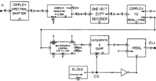
I-bit differential GFSK receiver: In the 1-bit non- coherent receiver the received signal is first passed through a spectral shifter, which fulfils the same function as a mixer. The Intermediate Frequency (IF) signal is then filtered with a Gaussian bandpass filter. In the implementation the received signal is shifted to baseband, thus a Gaussian lowpass filter can be used in place of a Gaussian bandpass filter in the simulation environment SPW, as seen in figure 3. This will not have any effect on the function of the detector. The BT- product in the lowpass filter is set to 1.0, which has shown to give the best BER performance for this implementation. The 'task for the 1-bit differential detector is to demodulate the signal from IF to baseband by multiplying the received signal with a delayed and 90" phase shifted version of itself. The following analysis is made assuming a real implementation. The signal after the predetection bandpass filter is of the form (3) where n(t) is the remaining additive noise due to the channel, a(t) is the amplitude after filtering, f, is the carrier frequency and @(t) is the information carrying phase. After lowpass filtering the product of the original signal and the delayed and phase shifted signal, the result at a time instant kT is on the form

d ( t ) = a ( t ) cos(2M t

+

@ ( t ) )

+

n ( t )

C

m

d (kT) = u(kr)u(kT- Z')sin(,

C

b .@ ))

+

2(kT)

(4)

as shown in [4] with the assumption that 27cfcT=2m, where n is an integer.

CY=--

bjOk

-

is the phase difference between the k'h and k-1 transmitted bit, and ii(kT) is the resulting noise. 00 represents the wanted signal for time instant

kT

and

e,,,

...

are IS1 contributions from previous and future bits. According to [4], the IS1 terms for j23 can be ignored. Eq 4 can then be expressed as

d ( k T ) = a(kT)a(kT - T ) sin(A@ )

+

A(kT)

1 J=-W J k - j

( 5 )

1 k

where

A@k=bk+2@-2+bk+1e-l+bk@O+bk-1e1+bk-282 ( 6 )

The sign of "=--b ,@ can be used to decide

what was sent. If the result is greater than 0 the decision made is that a 1 was sent, otherwise 0.

Differential D8PSK receiver: In the D8PSK receiver the carrier-phase is unknown, i.e. non-coherent detection, thus the signal itself is used as a carrier- reference. This fact combined with the differentially modulated signal make demodulation with a non- coherent differential detector effective. Coherent detection is not utilized for D8PSK modulation as described in [5]. As for the 1-bit differential GFSK receiver, the RMT measurements are made at the output of the differential detector.

1 " COMPLEL,

-

,..1 COMPLEX SHIFTER _" T O +++SPECTRALv

i.e. the signals for RMT measurements will be taken directly after the PLL.

BT

0.28 inf. (FSK)

Coherent GFSK Viterbi receiver: In the coherent receiver the signal is first passed through a noise reduction Gaussian filter with a BT product of 0.3 which has been shown in the simulations to give the best BER performance for this implementation. For relatively low SNR values, less then 10 dB, a matched filter should be utilized. The next step in the receiver is to feed the signal through the metric calculator, which calculates the costs to go to different states in the Viterbi block. In figure 5 is the coherent receiver structure shown.

e-2 0.1 00 e+1 0+2

0.13 8.22 28.29 8.22 0.13

0 0 45 0 0

Figure 3: 1-bit differential GFSK receiver. The D8PSK signal is filtered with a SRRC filter to narrow the bandwidth as described in [2]. This introduces ISI, which can be removed with a matched filter in the receiver. The receiver structure is shown in figure 4.

Figure 4: Differential D8PSK receiver.

The D8PSK standard slicer in figure 4 uses a differential detector in combination with an 8PSK slicer. The output of the differential detector is fed to the 8PSK slicer, which demodulates the phase change over one symbol to the corresponding three-bit sequence.

The differential detector for D8PSK is identical with the differential detector used in the GFSK non-coherent receiver.

Coherent Detection

For the coherent receiver, the reference carrier of the modulated signal must be recovered in order to demodulate the signal. This reference carrier can be obtained with a Phase Locked Loop (PLL). In this article a perfect carrier-phase recovery is assumed. Then the modulating signal is known and can be eliminated. This provides the base band representation of the signal and it is this signal that will be used for RMT measurements,

Figure 5: Coherent GFSK Viterbi receiver. Since the in-phase and quadrature-phase components of the GFSK signal are correlated, the detection has to be based on both components. In the metric calculator, the costs are calculated as the distance between the received and the possible phase states for the GFSK signal. GFSK with a BT product of infinity, i.e. without a Gaussian filter, has no IS1 and the phase contribution from every bit is 45 degrees. This will give eight different expected phase states, 0", +45", +90", +135" and 180°, assuming that the initial phase is 0". A BT product of 0.28 introduces ISI, which will smear the phase contributions over adjacent bits, as illustrated in table 1.

Table 1: Phase contributions (IN DEGREES) for GFSK and FSK, where go is the phase contribution from the

current bit and

&,

k = l , 2, is the phase contribution from the bit k bits away from the current bit. The contributions are positive if a 'one' is transmitted and

negative for a 'zero'.

From table 1 it can be seen that for Ikl > 1, the phase contribution is negligible. This results in that the phase contributions from previous bits will almost not influence the decision of the current bit since the lacking phase contribution is only 0.13" from the previous bit. When the current bit is received the accumulated phase is changed by 9.2

+

+

90 = 36.64". From this is it then possible to calculate the decision points for every state, the results are shown in figure 6. The decision points can be described as the points, which the received signal will be compared to. The output of the metric calculator will be the distances from the received signal to all the decision points.

Based on the phase states and the decision point pairs the trellis diagram in figure 7 is determined.

The Viterbi block makes the decision of which will be the next state from the output of the metric calculator. For each phase state, the Viterbi can only change state to the closest phase states. The Viterbi produces its output bits after that twenty steps, i.e. 20 bits, in the trellis has been calculated. 1 - 0.5 0 - b

.

p 0 Phase state

o, 2/4x ,* Decision point for slate

(daision. new stale)

1. 314: p. 1/4n 0, 34x, O ,I. 1/4n - 1. 4l4n 0. 4/4n t 0. 0/4n 1. 0/4n

*

0. 714n 0. 5/4n 1. 7/4n 4 . 5 0.5

Figure 6: Phase states and decision point pairs for each state.

RMT RESULTS

The GFSK and DSPSK modulated VDL Mode 4 signals used for calculating the time deviations for the different receiver structures have been generated in SPW. For all simulated receivers, the transmitted signal is multiplied with a frame sequence between the channel and the receiver in order to achieve VDL Mode 4-similar bursts, giving the effect that the correlations are made frame-wise. For correlation sequences longer than the 24-bit synchronization sequence for GFSK and the 48-bit synchronization sequence for DSPSK, the original bitstream is used to regenerate the undistorted modulated signals used for correlation. For the simulations in SPW, the signals are synchronized through all the blocks in the designs. This has the effect that the signals will be accurately sampled for all times, which provides perfect bit synchronization in the receivers. With a noise-free and non-distorted channel, the result of the correlation will give no deviation from the measured TOA, which in this case is the correct time instant. In the presence of a non-ideal channel, the difference between the measured TOA and the point in the interpolated correlation function giving the maximum result will give the deviation from the correct TOA, due to the channel distorting in the transmitted signal. In a practical implementation, where perfect bit synchronization is not possible, the calculated deviation from the measured TOA will give an estimate of the true arrival time, where the standard deviation calculated for perfect bit synchronization can be interpreted as an uncertainty- factor as a result of the channel.

The correlation algorithm has been applied to the signals using a Matlab function where the correlations for each receiver are made frame-wise for 1000 frames with different SNRs, and over different number of bits. The bit sequences beyond the initial 24-bit and 48-bit sequences for GFSK and DSPSK, respectively, have been derived from a random source. The different SNR values for each receiver are based on values to obtain BER values between approximately to This is an important consideration as for the non-coherent receiver designs the SNR to achieve a BER of lo4 will be significantly higher than that required for the coherent implementation [2]. Thus the TOA measurement for the coherent implementation can be interpreted to appear worse, however, this is only a result of the lower SNR values utilized. The coherent and non-coherent results should not be directly compared as a result of the significant differing SNR evaluated.

Received bit

( i i p p d l n w w hranch)

Figure 7: Trellis diagram for the Viterbi detector. The distortions that will affect the transmitted signals can be divided into different distinct channel properties. The distortions that are taken into account in the RMT simulations, in addition to AWGN, are CCI, multipath and Doppler frequency shift defined in [l, 31. All of these will influence the results of the RMT measurements.

Non-coherent GFSK Receiver

For the RMT results presented in this section, the different channel properties have been introduced individually, starting with AWGN and continuing through CCI, multipath and Doppler. In the case of CCI, multipath and Doppler, AWGN has also been incorporated into the simulations in order to achieve the appropriate SNR levels. The time deviations for each of the 1000 simulated frames are calculated for each separate channel property and the results are presented as

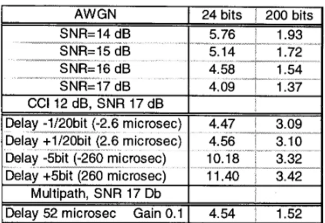
two-sigma errors. The results show that correlation over the whole burst gives significant improvements in terms of lower two-sigma errors, compared to correlation over only the 24-bit synchronization sequence. The correlation results for different SNRs and number of bits for the AWGN channel are summarized in table 2. It can be seen that increasing SNRs decreases the two-sigma errors. The results when incorporating CCI, multipath and Doppler are also summarized in Table 2 and it can be seen that those channel properties clearly affects the RMT results negatively.

According to Eq 2 a secondary timing two-sigma error of

1 ps would correspond to a secondary ranging two-sigma error of approximately 300 meters.

Table 3: Two-sigma errors in microseconds for non- coherent GFSK receiver.

AWGN

I

24 bits 200 bits

SNR=26 dB

I

1.81 0.68 AWGN SNR=14 dB S N R = I " ~ i B SNR=16 dB SNRz17 dB CCI 12 dB, SNR 17 dB Delay -1/20bit (-2.6 microsec) Delay+l/20bit (2.6 microsec) Delay +5bit (260 microsec)

Multipath. SNR 17 Db Delay -5bit (-260 microsec)

I

MultiDath. SNR 32 dB

I

I

1

24 bits 200 bits 5.76 1.93 1.72 5.14 4.58

__

1.54 4.09 2 1.37 4.47 j 3.09 4.56

---

II

-

3.10 11.40 3.42 xx I

10.18

-__I- j 3.32

IDelaV 52 microsec Gain 0.1

I

1.34 0.41

I

Doppler, SNR 32 dB

fd=280 HZ I 1.52 0.39

Coherent GFSK receiver

The received signal to be cross-correlated with the regenerated signal is taken at the output from the Gaussian lowpass filter of the coherent GFSK receiver implementation in SPW, shown in figure 5. At this stage the received signal consists of an in-phase and a quadrature-phase component. As is the case for the 1-bit differential GFSK detector the original bitstream is used for regenerating the GFSK modulated signal to be correlated with the received sequence. The correlation algorithm has in this case to be applied to both the in- phase and the quadrature-phase components for every burst. The two correlation functions for each burst are summed and the time deviation for the point giving the maximum correlation result is calculated.

As for the I-bit differential GFSK receiver the RMT simulations are performed for the specified channel properties, starting with AWGN and then adding CCI and multipath. Assuming a perfect PLL the Doppler frequency shift can be neglected for this receiver model.

As for the 1-bit differential GFSK detector 1000 bursts are simulated for each number of bits correlated over per burst and SNR value. As a result of the improved BER performance for the Viterbi receiver, the correlations are simulated for much lower SNRs compared to the 1-bit differential detector. The SNR range still corresponds to

a BER range from to 10". The RMT results for the GFSK Viterbi receiver are summarized in table 3 where it can be seen that the results for correlating over only the 24-bit synchronization sequences are poor, due to the low SNRs. For correlations over the whole burst the results are improved in terms of lower two-sigma errors.

Table 5: Two-sigma errors in microseconds for coherent GFSK receiver.

. . I

Delay 52 microsec Gain 0.1

I

4.54 , 1.52 As for the non-coherent GFSK receiver the RMT results when incorporating CCI and multipath are affected negatively. The two-sigma errors for the coherent receiver design can also be translated to ranging errors according to Eq 2.

Non-coherent D8PSK Receiver

The received signal to be cross-correlated with the regenerated signal is taken at the output from the matched SRRC filter in the D8PSK receiver implementation in SPW, shown in figure 4. At this stage the received signal consists of an in-phase and a quadrature-phase component. As for the two GFSK receivers the original bitstream is used for regenerating the modulated signal to be correlated with the received sequence. The correlation algorithm has again to be applied to both the in-phase and the quadrature-phase components for every burst. The two correlation functions for each burst are added and the time deviation

for

the point giving the maximum correlation result is determined.

For the D8PSK RMT simulations the different channel properties have been introduced individually, starting with an AWGN channel and continuing with CCI, multipath and Doppler frequency shift. For the CCI, multipath and Doppler simulations AWGN is also incorporated in order to achieve the appropriate SNR level.

The scenarios when simulating multipath and Doppler frequency shift are identical with the corresponding scenarios simulated for the 1-bit differential GFSK receiver.

The RMT results for the DSPSK receiver are summarized in table 4. The CCI level of 17 dB does not affect the two-sigma errors significantly. Multipath and

AWGN SNR=13 dB SNR=14 dB SNR=15 dB SNR=16 dB

I

1.02 0.74 CCI 17 dB. SNR 16 dB I 48 bits 240 bits 1.44 1.03 1.28 0.92 1.14 0.82

Delay -1MObit (-2.6 microsec) IDeIa; +1/20; (2.6 micros:

I

!ii

I

Delay -5bit (-260 microsec) 0.97 Dela +5bit 260 microsec 0.97

Multipath, SNR 16 dB

I

Delay 52 microsec Gain 0.1

I

1 . I 3 0.82

Doppler

I

fd=280 HZ

I

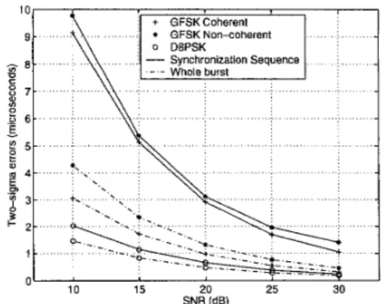
1.06 0.76

The RMT results vs. SNR when only incorporating AWGN is illustrated for all receiver designs in figure 8. The sigma errors when correlating over 24/48 bits as well as when correlating over the whole bursts are shown.

CONCLUSIONS

A number of simulations have been developed and implemented to evaluate the performance of RMT under a variety of channel conditions.

For the non-coherent GFSK receiver all RMT simulations which incorporate an AWGN channel, the results indicate that increasing the number of bits correlated over per burst and increasing SNRs will improve the timing results in terms of decreased two- sigma errors.

When incorporating multipath, Doppler frequency shift and CCI the RMT performance decreases in terms of higher sigma errors. CCI has the greatest negative affect on the RMT results. Although the coherent receiver has a much better BER performance [2] it still provides worse timing results when directly compared to the non- coherent receiver design. The basis behind this result can be simply explained as both designs are evaluated at SNR levels corresponding to a specific BER. The coherent design requires a lower SNR for the same BER as that obtained for the 1-bit differential detector. The RMT performance is strongly correlated with the received SNR of the signal. Thus, when the correlation algorithm is applied to signals distorted with higher noise levels, there is a negative impact on the timing results. When incorporating multipath and CCI the RMT performance decreases in terms of higher sigma errors. CCI has the greatest negative affect on the RMT results.

SNR (dB)

Figure 8: RMT results presented as two-sigma errors vs. SNR for the three different receivers.

Also for the DSPSK receiver all the incorporated channel properties decreases the RMT performance. CCI does not affect the RMT results as significantly as for the GFSK receivers.

A potential benefit of RMT is that the secondary timing performance can be directly translated to secondary ranging. A secondary timing sigma error of 1

ps corresponds to a secondary ranging sigma error of approximately 300 meters, assuming that the electromagnetic waves propagate through the atmosphere with the speed of light.

REFERENCES

VDL Mode 4 Standards and Recommended Practices , Version 6.0.0, September 17 1999. Nilsson, H. et al, “Study on the options for time synchronization in the VDL Mode 4 Datalink System“, December 1999.

Fiebig, U-C; Haas, E; Hoher, P; Lang, H, “Future VHF architecture implementation study WP 5000: Physical layer final report”, May 1999

Yongacoglu, Abbas; Makrakis, Dimitrios; Feher, Kamilo, “Differential detection of GMSK using decision feedback”, IEEE Transactions on Communications, vol. 36, no 6, p 641-649, ISSN 0090-6778, June 1998. Couch, Leon W 11, “Digital and analog communication systems”, 3:d edition, New York: Macmillan, ISBN: 0-02-325391-6, 1990, pp. 547-551.