VT1 notat Nr 76-1994 Titel: Författare: Resursgrupp: Projektnummer: Projektnamn: Uppdragsgivare: Distribution: Also Published as:
Utgivningsår 1994
Implementation of a Traffic Assignment Algorithm in a GIS-T
Kjell Johansson
Transporter och samhällsekonomi
50015 .
Implementation of a Traffic Assignment Algorithm in a GIS-T KFB Fri "LIU-MAT-C--94/20--SE" div Väg- och transport-forskningsinstitutet &
IMPLEMENTATION OF A TRAFFIC ASSIGNNIENT ALGORITHM IN A GIS-T
Examensarbete av
Kjell Johansson
November 1994
LIU-MAT-C--94/20--SE
Also Published as: VTI-notat Nr 76-1994
Department of Mathematics Linköping University
Acknowledgements
I thank my supervisor Sakis Migdalas at the Department of Mathematics at Lin-köping University.
For the ñnancial support I thank The Swedish Transport and Communication
Research Board (KFB).
I also thank Jan Eriksson, Urban Björketun, Henrik Jönsson and all the others at the Transport Economics, Swedish Road and Transport Research Institute, for all your help and the lovely atmosphere at work.
Special thanks to all my friends and relatives, and especially Benny Pettersson & Sussie Ahlén, for your support during my studies at Linköping University. Finally I thank my family for all their love and support during these years of studies.
Linköping, November 1994 Kjell Johansson
Foreword
Because of its practical importance and the size of real life problems, the
develop-ment of algorithms for the solution of the traffic assigndevelop-ment problem is a very inte-resting and active research topic.
In February 1992, Michael Patriksson & Torbjörn Larsson (both Linköping Uni-versity, Department of Mathematics) published an article in "Transportation Sci-ence, vol. 26", where they presented an algorithm for the solution of traffic assign-ment problems. This algorithm is called "Disaggregated Simplicial Decomposi-tion". The algorithm has so far being running on VAX-computers and Sun Work-stations, but since the PCs are getting faster and with larger memories, there was a wish to convert the program into a PC-compatible program.
The task has been to :
- Make the program easy to understand. This involved getting the program
well structured, rename the variables into suitable international names,
add comments and remove all unnecessary variables and programming steps.
- Enable the execution of the program with either double or single precision variables. The original program used doubleand double-double precision variables, one was not able to make the calculations in single precision. - Implement the program into a GIS-T (called TransCAD). This gives,
among other things, the possibility of getting a visual picture of the results. All the above have been done and the tests show that the PC-compatible program gives good results. (For the network of Barcelona, relative errors less than 2% has been reached for single precision and for double precision less than 1%.)
Some improvements of the program has been suggested, and they are:
l. Implement the program in Fortran 90 instead of Fortran 77, i.e. use the new commands and intrinsic functions.
2. Try to get the EXE -ñle smaller so that bigger programs may be run un-der DOS. Running program unun-der DOS (instead of Windows) makes the runtime smaller. All compilers can not create Windows compatible EXE-files and then problems with a size of the Barcelona network can not be solved with the present PC-compatible program.
3. To get the program even more easy to understand, the sorting (in
MSTCOM, the subroutine that solves the master problem) can be put in its own ñle. More comments can also be added.
Contents
1. Introduction . . . . 4
1.1 The Transportation Network 4
1.2 Transportation Models . 6
2. Traffic Assignment . . . 8
2.1 Different Types of Assignment . 9
3. A Mathematical Formulation of the Traffic Assignment Problem . 10
4. The Frank-Wolfe Algorithm . . 11
5. The Implemented Algorithm . . 13
5.1 Theory . . . . 13
5.2 The Algorithm . . . 14
5.3 Comments About the Implementation . 16
6. Changes and Improvements . . 17
6.1 Cleaning up the Program . 17
6.2 Comments . . 17
6.3 Time Calculations . 17
6.4 Method of Gill-Möller . . . . 18
6.5 The Sorting in the MSTCOM-subroutine . 18
6.6 Saving of the Routes . . . 19
7. The Converting Program . . 20
7.1 How the Program Runs . . 20
7.2 The Converting . . 20
7.3 The Split-up . . 21
8. Implementation in GIS . 22
8.1 The Implementation . . 23
8.2 The Export Procedure . 24
8.3 The Import Procedure . 25
8.4 The TCCONV-program . . 25
8.5 The Result . 25
9. Comments Regarding Fortran 90 . . 27
9.1 Some of the News . . 27
9.2 Fortran 77 vs. Fortran 90 . . 28
10. Tests . 30
11. Discussion . . 32
References . . 33
1. Introduction
1.1 The Transportation Network
Since the demands on the transportation systems continuously increase, it is neces-sary to look for different changes, in e. g. network infrastructure, in order to meet new demands. Examples of these demands are high levels of safety, accessibility, envi-ronmental quality and economic efficiency.
Examples of the changes are:
If we cut down on the public transportations, what will happen with respect to the current traffic situation?
If we try to regulate the traffic harder, what will be the reaction of the network users?
What will happen if we build a new road between A and B? Will there be a con-siderable change in travel patterns?
- If there is an increase in population or car ownership. What will the changes in traffic patterns be?
If a number of factories in an area are shut down, what changes in the traffic pattern will that give rise to?
To make suitable analyses we use mathematical models, which are suppose to sim-ulate the real transportation system as close as possible.
The transportation system is described by a network, which consists of a set of nodes and a set of links (connecting the nodes).
The links represents roads, Streets & public transportation lines, while the nodes corresponds to intersections. origins, destinations and/or points where a change in the road conditions occurs. There is an example of a network in Figure 1.1
Gvöø
D
Figure 1.1: Example of a network
O = Origin node , D = Destination node , I = Intersection node
Every link has a congestion function, that tells how much it costs to use the link (de-pending on the actual flow of the link). This function can for instance be a time func-tion, which tells the cost in time to use a certain link. The bigger flow, the bigger cost (it takes longer time to travel on the link if there is a lot of traffic).
A congestion function is depicted in Figure 1.2.
120 100 --80 -h 60 --Ti me (s ec on ds ) 40 «-20 v
0 1000 2000 3000 4000 5000 6000 7000
Traffic Volume (vehicles/hour)
Figure 1.2: A congestion function.
The reason why the function increases so rapidly after a while is that it starts to reach the point where a jamming is close at hand.
1.2 Transportation Models
The transportation models are usually divided into two types. The first type consist of the supply models which deal with questions like how the suppliers respond to certain demands of transportation. The second type of models are the demand mod-els. This type deals with questions like how the road users react to the amount of service and the size of the costs in the transportation system. The reason why the terms supply and demand are used is because one looks at the transportation system
as a market.
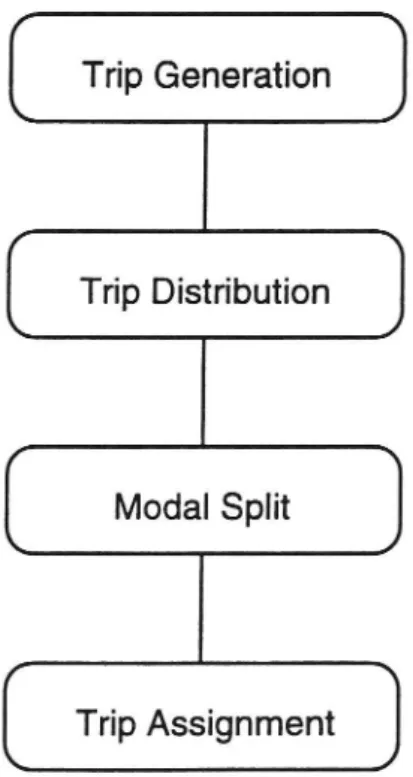
The second type of models (demand models) are often divided into a four-step mod-elling process, which consists of four sub-models. These sub-models are: trip gen-cration, trip distribution, modal split and trip assignment. The models are to be con-sidered in the order given by Figure 1.3. The results of one model are the indata to the
next sub-model.
Trip Generation
Modal Split
[ Trip Distribution
[ Trip Assignment ]
Figure 1.3: The four sub-models
The first sub-model, trip generation, deals with the "production" and "attraction"
of each zone in the transportation system. In other words, the sub-model tells how much input and output each zone creates/demands.
The trip distribution allocates trips from origins to the destinations, i.e. an origin/ destination matrix (OD-matrix) is created. This OD-matrix tells the trip relations between each zone. An example of an OD-matrix is given in Example 1.4
Example 1.4:
0 32 21
A 3x3 OD-matrix is given by: 17 0 38
25 13 0
This means that there is a demand of 32 from zone 1 to zone 2. The demand from zone 3 to zone l is 25, the internal demand (1 to 1, 2 to 2, 3 to 3) is 0 in all cases.
The modal split deterrnines the shares of each different transportation mode, based on the total number of trips for each OD-pair. The two most interesting modes are the public transportation and the private cars.
The fourth sub-model, trip assignment, is also called traffic assignment. What the model does, is to assign the traffic (the trips) on routes between the origin and des-tination zones. It is this model that the program of Michael Patriksson & Torbjörn
Larsson deals with.
The four step modelling process is illustrated by the following example.
Example 1.5:
The Peterson family live in Stockholm and they are discussing what to do on their holiday. They decide to make a trip (the trip generation is done). After a long argument they decide to visit some friends in the lovely town of Linköping (the trip distribution is ready). To have the biggest flexibility they choose to use their own car (modal split). And when the discussion of route come up, thefinal agreement is to make a detour via Örebro to see a football game (the trip assignment is done).
2. Traffic Assignment
Because of the size of real life problems and the practical importance, the develop-ment of algorithms for the solution of the traffic assigndevelop-ment problem is a very inter-esting and active research topic. If we can solve the real life problems effectively, the improvements to the traffic conditions can be done faster and easier. There is also a challenge to develop efficient algorithms for this kind of models (very large and highly structured) and challenges are what many scientists (and especially the mathe-maticians) love to work with.
As previous mentioned each link has a function that tells the cost of using the link
(depending on the actual flow of the link). Mostly the cost equals the time that it
takes to travel on the link. These functions are called volume delay functions, link performance functions or congestion functions.
The functions are non-linear and strictly increasing (the travel time increases if the
volume of traffic, on the link, increases). An example of a volume delay function is
shown in Figure 1.2.
Two main principles where stated in 1952 by Wardrop ("Wardrop conditions"),
and these are:
Wardrop's first principle
The travel time on all used routes are less than or equal to the travel times on the unused ones.
Wardrop's second principle
The average travel time is a minimum.
If the first principle is fulfilled, no user can get a lower travel time by altering his
(her) route. Every traveller has minimized his (her) travel time. This is often
re-ferred to as the user equilibrium.
If the second principle is fulñlled, the total travel time is minimized. This is the best solution for the society and is often referred to as the system equilibrium. One of the ways to reach this optimum (for the society) is the use of regulations. The only time when the above optima are equal is when we have a congestionfree traffic situation and that is the ideal traffic situation.
2.1 Different Types of Assignment
As the title above indicates there are different types of assignment, and below three of them will be described shortly.
All or nothing assignment, as the name implies each route is either given all the flow or no flow. This is done by calculating the shor-test route and then assigning all of the flow to that route. This is not a good solution because the loading on the route will be heavier than before.
Incremental assignment, this type of assignment divides the given flow into N equal parts, where N is any number greater than or equal to 1. (If N=l we have an all or nothing assignment.) Then N all or nothing assignments are done, each time assigning one Nzth of the flow to the shortest route Equilibrium assignment, this type fulñls Wardrop's first principle. It means that
there can not exist any unused route cheaper than the ones used. This assignment can be solved by using the
3. A Mathematical Formulation of the Traffic
Assignment Problem
One of the ways to formulate the traffic assignment problem will here be presented. First some deñnitions:
G = (N, A) - The network where N is a ñnite set of nodes and A is a fmite set of arcs.
C - The set of commodities, defined by origin and des-tination pairs (p, q). C c NxN
(p, q) - An origin-destination pair. dpq - Demand between OD-pair (p, q)
fapq
-
Flow from origin p to destination q through are a
(p, q)e C , ae A
fål
-
Total flow on arc ae A.
ga(fa)
-
Arc performance functions, the travel cost on arc
ae A.
Wi
-
Set of arcs initiated at node i.
Vi
-
Set of arcs terminated at node i.
And now the model:
[TAP]
min 'rm = 2 g.(fa)
(1)
aeA dpq , if i = p
s.t.
Zain-:fam =
--dpq ,ifi=q
(2)
aewi
vi
0
, otherwise
V ieN , V (p,q)e C
2 fapq = fa
V ae A
(3)
(p.q)eCfapq _>_ 0 V aeA , V (p,q)e C (4)
The objective (l), that we want to minimize, is the sum of the arc performance
functions for each arc. The first condition (2) makes sure that all demands will be performed . Next condition (3) checks that the sum of all flow on an arc equals the total flow on the arc. The last condition (4) makes sure that no negative flows
appears.
4. The Frank-Wolfe Algorithm
If we use the Frank-Wolfe algorithm on the above formulation, it will be like this:
The upper index (k) indicates how many iterations that have been performed. Oo Initialization
Find a feasible solution fm). This can, for example be done by
using all or nothing assignment on free-flow travel times (at zero flow). Define stopping criterion ( 81 - max. relative error,
8,2 - minimum of improvement, 8,3 - min. demand on the
step-length). Set initialvalues on the lower and upper bound: LBD=oo and UBDz-oo.
lO Linearization
Linearize the objective with the help of first order Taylor ex-pansion in the neighbourhood of tm.
100 = Tum) + VkaöT - (y - tm)
20 Generation of the Search Direction
Solve the following linearized subproblem:
[LP]
min ny) = Tum) + VT<t*'° T - (y - tm)
dpq ,if i = p
s.t. Zyam-Zyapq = -dpq ,ifi=q
aeWi aeV-l .
O , otherw1$e
VieN , V (p,q)e C
zyapq = yZl V aEA
(qu)eC
ynpq _>. 0 VaeA , V (p,q)e C
30
40
50
60
This is equivalent to a cheapest route problem with arc costs
g ; (fam) . The solution to the problem corresponds to Cheapest
(k)
route flows. This solution equals a point S' which gives a lower bound I( i'm) on the optimal objective value. The lower
bound (LBD) is updated if the new value is greater than the
current lower bound, i.e. LBD = max{ LBD, I( SIM ) ;.The
search direction: dm = SIM- Fk).
Convergence Test
Check if the relative error is small, i.e.
(ram) - LBD ) / UBD < 2,
If this is fulñlled, terminate with a near-optimal solution fm.
Line Search
Solve the following line search problem:
min T(h) = T(f°°) + h-($'(k)-f°°)
h6[0,1]
The solution equals a steplength hm.
New Iteration Point
The new iteration point is calculated as:
f(k+1) = f(k) + ha:) . (y(k)_ tm)
The upper bound is updated if T(h) is less than the current upper
bound (UBD), i.e. UBD = min { UBD, T(h)
Convergence Test
Check the relative error:
(TOM) - LBD) / UBD < 81
Check if the objective value has improved enough:
( T(Fk+')) - T(f ° )) < 82
Check if the steplength is to small: h(k) < 83
If any of the above criterion is fulñlled, then terminate with a
near-optimal solution for the [TAP]. If none of the above is fulñlled,
let k=k+1 andgoto 10.
5. The Implemented Algorithm
The Frank-Wolfe algorithm is an efficient algorithm in the first iterations, but in the later iterations it is characterized by zig-zagging. This makes the convergence slow, i.e. a very large number of iterations is usually required to obtain a specified precision. Moreover, the improvements may be diminishing small and if the preci-sion is high, it may never be reached. Another drawback is that the algorithm might generate cyclic flows, and optimal solutions can not contain cyclic flows.
Because of these drawbacks Patriksson & Larsson choose to implement the
BSD-algorithm to solve the traffic assignment problem. It is the DSD-algorithm that the program of this work deals with.
First we take a look at the theory, then we look at the algorithm and finally there are
some comments about the implementation of the algorithm.
5.1 Theory
Let us once more take a look at the [TAP] problem. We see that almost the entire
feasible set, for the problem, is a Cartesian product with respect to the
commodi-ties. In other words the matrix of constraints has a block-diagonal shape. How a block-diagonal shaped matrix looks like can be seen in Figure 5.1.
(X
\
\
X)
Figure 5.1: A matrix of block-diagonal shape.
Suppose that we know a nonempty subset of the set of simple routes lim , for each commodity (p, q). All routes i in lim are related to a convexity variable km, , which will denote the portion of demand dpq distributed along route i. Let ?tm be the vector of convexity variables Ämi for all ie Fm , and let the vector ?t consist of all such ?t . The arc flows fa can be calculated from the weighted route flows in the following way:
fa = 2 dpq zömiakmi (5)
(p.q)eC iequ
Here the ömia is an element from an arc-route incidence matrix (ömm) for G,
i.e. (ömm) = 1 if route re qu contains are a (otherwise (ämm) = 0).
Through (5) the function T(f), in [TAP], will be a function of the convexity
vari-ables 7» and because of that we write TO.) instead of T(f). The restricted master problem (for [TAP]) will now be as follows:
[RL/IP] min TOt)
st. 2 km, :1
V (p, q)eC
ioslâpq
?tmi 20 Vielâpq , V(p,q)eC
5.2 The Algorithm
Here the DSD-algorithm will be described. The DSD algorithm is an iterative proce-dure similar to the Frank-Wolfe algorithm. The basic strategy is to iteratively gener-ate and store shortest routes, and solve the problem over the routes currently stored. What the algorithm of Patriksson & Larsson does is that it uses a scaled reduced gradient method to find a near optimal solution. Then it uses a second order method to get a better solution. The second order method used is a constrained Newton algo-rithm. The reason why two methods are used, is that the first one (scaled reduced gradient) has a slower convergence if a very high accuracy is required. The reason of the slow convergence is that the method is a first order method. First we take a look at the scaled reduced gradient method, especially adapted to [RMP].
O0 Initialization
Find a feasible solution FO). This can be done with a number of
in-cremental assignments. Define Stopping criterion.
l0 Search Direction Generation
As basic variable ipq for commodity (p, q), choose the one with
. ^ . . (k)
the largest ?tmi for all 16 qu , 1.e. ime arg max{ lm, ]. Let Npq denote the set of nonbasic variables for commodity (p, q). Compute:
rpq = VNpq T(Ä °) - Vipq T(7t °) - 1
where every component of VTOJ'O) is calculated in the
follow-ing way:
VW» = d,q 26mm gaf?)
aeA
The calculation is done with the help of (5), which deñnes the
aggregate arc flows fam.
The vector of all rpq is the reduced gradient The negative of a scaled reduced gradient defines the search direction as follows:
- . . i n i . <
_(k) Spql rpql if 1 ;t 1pq and rpql _ 0
I =
?JU
mi spqi rpqi 1 1'f ' :'
lpq an rpqi >d
0
-(k _ -(k
iatim
where S = diag(qui) is a positive deñnite scaling matrix. To deflect the search direction away from near-active non
neg-ative constraints we use Nä; , which is a well known
tech-nique.
20 Convergence Test
If rm = 0 : terminate Nk) solves [RMP].
3O Line Search
Solve the line search problem:
[LS]
h min ] M) = T(Ã. °+h - rm)
Nk).
where:
hmax = min min { -j'g- : få:) < 0%
(p,q)eC i<=.Rpq rpqiThis gives the solution hm, where hm is a steplength.
40 New Iteration Point & Convergence Test Let Nk) = 76 + ha - P
00-Check the stopping criterion (defined in 00) If any of them is fulñlled, Nk) solves [RMP] approximately. If none is fulfilled k=k+ 1.Goto 10.
Now we take a look at the second order method, a constrained Newton algorithm. The subproblem is approximated, at each iteration point, by using only the diago-nal of the Hessian matrix. Due to this approximation of the Hessian, the quadratic programming subproblem is separable into:
[QPS]
min
{apqi (kw 4(ng ) + åbmi (Ami mg; f]
IEqu
s.t.
:Kpm :1
105qu
Where
apqi = dpq Z öpqia g;(fa(k))
aeA
bmi = då, 2 öm g;'<f;
aeA
This problem is analytically solvable at low computational cost. It is done by Lagrangean dualization of the convexity constraint together with a line search on the piecewise quadratic one-dimensional dual function. The line search is done by studying breakpoints of the piecewise linear derivative.
5.3 Comments About the Implementation
In the program, the calculation of shortest paths is done with an implementation of Dijkstra's algorithm.
The starting point (step 00 in the scaled reduced method above) is found by solv-ing a number of incremental assignments.
The line search is solved by an approximate Armijo-type line search, this is done due to the disadvantage of solving it accurately.
Each volume delay function is of the following typez oc x + B XC , where on, [3 and c are known a priori.
6. Changes and Improvements
6.1 Cleaning up the Program
Since the program has been tested in many ways and for different purposes it con-tained several variables and a few loops that where meaningless. These variables and loops where removed.
The variable names where exchanged to international suitable names. They also have the same meaning in all parts of the program (which was not the case before). To eas-ier know what each variable means, an explanation is found in the beginning of each procedure. The structure was only slightly adjusted. The biggest changes was to re-move as many GOTO-sentences as possible and to let all programming parts be writ-ten in capital letters. This was done in order to increase the readability of the program.
6.2 Comments
Since the program was a bit hard to understand, due to the lack of comments in some places, more comments where added. It can be hard for a programmer to know how much comments he/she should use. Everything might seem obvious for a person who has worked with a program for days (often months). But is it as obvious in a year, or for a person who has not worked with it? Probably not, and therefore as many corn-ments as possible should be written. It might take a few minutes longer in the pro-gramming process, but there can be hours to earn in a "further deveIOpment process" and even in the testing phase.
6.3 Time Calculations
Instead of having the time calculations in place, a subroutine (called TIME) that makes all the necessary calculations has been created. This makes it much easier to insert such a calculation. It is a lot easier to write the call of a subroutine than to write all the needed steps. The time functions are examples of functions/commands that can be different from one compiler to another. Because of that one might have to change the functions/commands in the subroutine, and it is preferable to make changes
in only one place (a subroutine), insteadof several places (each place where the time-calculation is needed).
6.4 Method of Gill-Möller
When a scalar product is calculated there can be a signiñcant loss of precision. In attempt of trying to avoid that, the method of Gill-Möller has been implemented in all places where a scalar product is calculated.
The method of Gill-Möller is used like this:
The scalar product wanted is: RO = XTG
The method uses two important variables: RO and T1.
RO contains the calculated scalar product between the vectors X and G. T1 contains the sum of all losses made in each iteration.
In short terms, the method keeps track of all the losses in significance, and in the end all losses are added to the scalar product calculated.
Programming-method:
R0=O
Tl=0
DO lOO I=l, VECTORLENGTH
T3=X(I) *G(I) T2=RO+T3 T1=Tl+ (T3- (T2-RO)) RO=T2 lOO CONTINUE RO=RO+T1
First the variables RO and T1 are zeroed. After that a DO-loop, over the vectors X and G is entered. A value (T3) for the multiplication of the current vector elements
is calculated. Then the total scalar product so far (T2) is calculated. The loss of sig-nificance in this step is calculated and added to the earlier losses (T1). The last step
in the DO-loop is to update RO (the scalar product). When leaving the loop there is
only one step left, and that is to add the losses (T1) to the variable RO.
6.5 The Sorting in the MSTCOM-subroutine
(subroutine for solving the master problem)
During the time for this work, Henrik Jönsson (Swedish Road and Transport Research Institute) has improved the sorting. He has used IF-sentences for all cases when the number of roads is less than or equal to 4. If the number of roads is greater than 4, a sorting routine named HPSOIÖ (written by Roy E. Marsten, Dep. of Management
Information Systems, University of Arizona) has been implemented. Since there are
some questions whether this routine can be used outside the University of Linköping
(on account of license agreement) the choice to use the old sorting, in the cases when
the number of routes is greater than 4, was made.
6.6 Saving of the Routes
During the time for this work, Henrik Jönsson & Pontus Matstoms (both of the Swed-ish Road and Transport Research Institute) have improved the saving of the routes.
Earlier each new route was placed (saved) last in the routevector, which made the
vector very large. The idea of the improvement is to use earlier saved routes, if pos-sible, and thereby cut down the size of the routevector. A detailed explanation of this can be found in a forthcoming issue of "VTI-Notat". In tests done so far it seems that the vector can be reduced to only 25-50% of its original length.
7. The Converting Program
To make the convertion between single and double precision easier, a program that converts the original PC-program (into the wanted precision) has been created. This
program also splits the original PC-program into smaller parts, where each part
con-sists of a subroutine or a function. Thereby all subroutines/functions becomes a file of their own. This can be useful when there is need of testing a new part or a new
improvement. It is much easier to find a certain place in a small file/program, than
in a large one. Another advantage is that one can do all kinds of tests in the small
programs and still have the original PC-program unchanged.
7.1 How the Program Runs
The program begins with a question of the file to convert (including the extension). After that, a question of the precision wanted is asked. Then the program converts and splits up the file.
7.2 The Converting
What the converting program does, is that it reads one line of the original PC-pro-gram. If the line read starts with "CS" or "CD", it indicates that the following line/
lines are specific for single precision (CS) or double precision (CD). The number of
lines that are of single/double precision is found in position 3 and 4.
If the precision read does not accord to the input precision, a "C" will be written in position 1 for the lines not corresponding to the latter precision. That is, these lines will be marked as comments and will not interfere when the resulting programs are executed An example of how the converting program makes the converting can be seen in Example 7.1.
Example 7.1
The program (a part of it) to convert looks like this: CD2
C DOUBLE PRECISION X, Y
C DOUBLE PRECISION DIVIDE
C82
REAL X, Y
REAL DIVIDE
If the wanted (input) precision is Double, the converting program performs the following steps:
First it reads the "CD2" which tells that the next two lines are specific
for double precision. Since the wanted precision is double, a blank " "
will be written in position 1 in the next two lines.
The program copies the following two lines with only one change, the "C":s in position l are removed and blanks are written instead.
In the fourth line the program finds "C82", which tells that the next two lines are specific for single precision. Since the wanted precision is dou-ble the next two lines are copied with only one change, a "C" will be writ-ten in position 1. The output of the program will then be:
CD2
DOUBLE PRECISION
X, Y
DOUBLE PRECISION
DIVIDE
C52
C
REAL
x, Y
C
REAL
DIVIDE
7.3 The Split-up
If the letters in position 1 and 2 are "CB", they indicate that in the next line a new
subroutine/function starts.
The program will then close the file, that it is writing on, and a new file (for the new
subroutine/function) will be opened.
The name of the new file (excluding the extension) is found on the same line as the "CB", starting in position 4. An extension (.FOR) is automatically added to the
file-name. The number of letters in the ñlename is found in position 3.
The writing on the new file will then continue until "CB" or "CE" is found.
If "CB" is found the previous steps will be performed again. If "CE" is found, it indi-cates that the end of the original PC-program has been reached, and the converting program terminates.
How the Split-up works can be seen in Example 7.2.
Example 7.2
The program (a part of it) to convert looks like this:
END CB4TEST
SUBROUTINE TEST(X, Y)
The first line (END) is the end of a subroutine.
The second line (CB4TEST) is the line that gives the information (to the
con-verting program) that the next line is the start of a new subroutine, and that the
name of the new routine is TEST.
The third line (SUBROUTINE TEST (X, Y) ) is the start of the subroutine
TEST.
A complete listing of the converting program is found in Appendix 1.
8. Implementation in GIS
GIS stands for Geographic Information System, and is a system where information related to geographical objects can be stored and presented. To get the information stored one can point at the object and the data will be shown on the screen.
One could say that a GIS-map is a map with information (an intelligent map) in-stead of just being a map.
The GIS used in this work is called TransCAD, and it is a GIS-T. The T stands for transportation and it means that it is a GIS especially made for use within the traf-fic and transportation area.
TransCAD has an amount of procedures for transportation related calculations, which is one of the reasons it is a GIS-T and not only a GIS. There is also a possi-bility of creating your own procedures and interface them with TransCAD.
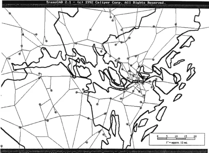
Below there is an example of a map, taken from TransCAD. The map shows the lake Mälaren and Stockholm.
Figure 8.1: Map showing the surroundings of the lake Mälaren and Stockholm.
8.1 The Implementation
The possibility of implementing the traffic assignment program of Michael Patrik-sson and Torbjörn LarPatrik-sson and get a visual picture of the solution is very inte-resting ("one picture tells more than a thousand values"). Therefore a new version of the result subroutine was written. This version creates an outdatañle that is in the format wanted by TransCAD when data is imported.
Two small procedures (interfaces) has been created in the TransCAD procedure
toolkit. These interfaces makes it possible to export data from TransCAD and import the results from the traffic assignment program.
8.2 The Export Procedure
This interface starts with a command that makes the database to remain open during the run of the interface. Next the graphics display is saved before the rest of the procedure is run. The third step is to check that the layer is set to links, if this is not so then it will be done automatically. Now the data is dumped. The data is in the following format:
From-Node , To-Node, Alfa , Beta , Exponent
Alfa, Beta and Exponent deñnes the volume delay function as defined in section 5.3. The ñfth step is to convert the outñle (containing the dumped data) into the filestruc-ture wanted by the traffic assignment program of Patriksson & Larsson. This is done
with a program called TCCONV (see section 8.4). At last a BAT file is run.This file
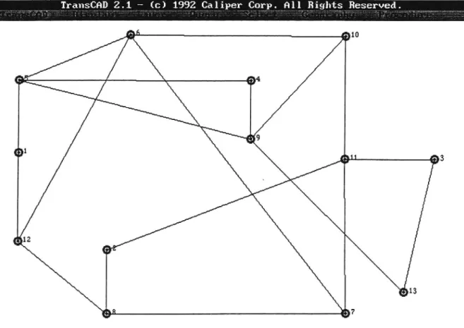
copies the new data-file to the directory where the traffic assignment program is run. The export procedure can be found in Appendix 3 and a picture of a network (the
Nguyen network , the network can be found in Nguyen & Dupuis) from TransCAD can be found in Figure 8.2.
6 10
Figure 8.2: The bare network.
8.3 The Import Procedure
This interface starts with the same three steps the export procedure does: the data-base is set to remain open, the graphics display is saved and the layer is set to the link layer (if this has not been done already). The next step is to copy the resultñle from the directory where the traffic assignment program works to the TransCAD directory. Finally the file is imported.
The import procedure is found in Appendix 4.
8.4 The TCCONV -program
The program has two indatañles, one containing the OD-table (called
'TASSOD.TBD') and the other containing the linkdata (called 'OUTFILE.DAT'). The outputñle is called AADATADAT and contains all the commodity data, node data and link data. There are two files used within the program. They store only the interesting data from 'TASSOD.TBD' respective 'OUTFILE.DAT'. These ñles are called 'COMFILEDAT' (used for the commodity data storage) and
'LNKFILEDAT' (used for the link data storage).
The program reads the TASSOD-ñle, gets rid of everything that is not wanted, stores the remaining data in 'COMFILEDAT' and calculates the number of com-modities. Then the interesting data in 'OUTFILE.DAT' is stored in a file called 'LNKFILEDAT' and the number of links is calculated. The highest node number (node-ID) is found by going through the LNKFILE. Finally the AADATA-ñle is created. First the number of links, nodes and commodities are written Then the commodity data are copied from 'COMFILEDAT' and the linkdata from the 'LNKFILEDAT'-ñle.
The complete program is found in Appendix 2.
8.5 The Result
An example of a result from the algorithm of Patriksson & Larsson can be found below in Figure 8.3. The picture shows the solution (the flow pattern) of the net-work shown in Figure 8.2.
TransCHD 2.1 - (c) 1992 Calipeerpr .väll Rights Reseryed.
X1112.24?
Figure 8.3: The network with flow patterns.
9. Comments Regarding FORTRAN 90
The international standardization board has accepted Fortran 90 as a new standard, ISO 1539-1991, thus Fortran 77 is no longer the standard. Because of that a few comments on some of the news in Fortran 90, that can be of use in the traffic
assignment program of Patriksson & Larsson, will follow.
9.1 Some of the News
In Fortran 901ine-numbers should be excluded (for use only in exceptional cases). To make that easier there are some new commands (1-2).
1. The termination END DO has been introduced in the Do-loops. In Fortran77 (when using a Do-loop) there has to be a line-number. But now the Do-loop can end with END DO, and the line number is not needed.
To make the program easy to understand one can give names to every Do-loop (a good suggestion if the program contains Do-loops within Do-loops).
2. Other new features are the EXIT and CYCLE commands. The EXIT-command makes it possible to jump out of a Do-loop before the loop has ended. In other words, one does not have to use a GOTO-command to jump out of the loop. The CYCLE-command jumps to the next iteration of the current Do-loop. Example on the use of the commands END DO, EXIT, CYCLE is shown below.
Example9.l BIG : DO I = 1, 12 A = A + I SMALL : DO J = 1, 10 IF (I < J) CYCLE BIG LEFT(I,J) = MATRIX(I,J) END DO SMALL IF (I = 10) EXIT BIG END DO BIG
In this example a jump out of the Do-loops will be done if (I = 10). In the inner Do-loop a jump to the next outer cycle will be done when (I < J).
3. Another new command is the CASE-statement. By using this one does not have to use a number of IF-statements. An example of the CASE command is shown below.
Example 9.2
SELECT CASE (I)
CASE (:-l) WRITE(*,*) 'Negative' CASE (O) WRITE(*,*) 'Zero' CASE (1:10) WRITE(*,*) '0 < I < 11' CASE DEFAULT WRITE(*,*) 'I > 11' END SELECT
Fortran 90 also contains a number of new intrinsic functions. Three of them are:
DOT_PRODUCT - Calculates the scalar product between two vectors (which have to be of the same length).
MATMUL - Calculates the matrix product between two matrixes (which have
to be consistent, i.e. the dimension have to be of the type (LJ) for one and (J,1) for the other).
TRIM - Deletes the ending blanks in a text string.
9.2 FORTRAN 77 vs. FORTRAN 90
Nothing that exists in Fortran 77 is removed in the new Fortran 90 version. How-ever aconcept called obsolescent is introduced. It means that certain constructions may be removed in the next version of Fortran. These constructions are:
- Arithmetic IF-statement.
- Real or Double Precision variables enclosing DO-loops. - Terminating several DO-loops at the same line.
- Terminating a DO-loop in any other way than with CONTINUE or END DO - PAUSE
- ASSIGN with "assigned GOTO" and "assigned" FORMAT - Jump to END IF from an external block.
- Hollerith constants in FORMAT, i.e. editing with: nHtext
- Alternative returns.
Our program does not contain any arithmetic IF-statements, all variables in the
Do-loops are integers and all Do-Do-loops terminates on different lines and with the
state-ment CONTINUE. This makes it possible to remove the first four constructions without effecting the program. The next four constructions can also be removed since neither one of these has been used in the program. The last construction can also be removed since the program does not have an alternative RETURN from any routine. The subroutine MSTCOM had an alternative RETURN but a GOTO has replaced the need for two RETURNS.
10. Tests
Here the results from some of the tests will be presented. The tests have been per-formed on two different test networks (the sizes of the networks are shown in
Table 10.1). The PC used in the tests is a "Compaq Deskpro 5/60M".
Network Nodes* Links* Commodities*
Nguyen 13 19 4
Barcelona 1020 2522 7922
Table 10.1: Sizes of the networks.
(* Number of Nodes/Links/Commodities)
We start by performing a couple of tests to see if the PC-program reaches near-optimal solutions. We look at the objective value,lower bound & relative error and compare the PC-versions (single , SP, and double precision , DP) with the
VAX-results of the original program. Each table below (Table 10.2 - 10.5) represents a
cer-tain network (the first two: Nguyen, the next two: Barcelona) and a cercer-tain bound on
the relative error (8).
PC, SP PC, DP VAX
OBJ 8505439 850543642 85054.1585
LBD 8438123 843812344 843555847
8 79776 E-3 7.9772 E-3 82813 E-3
Table 10.2: Nguyen, 8 _<_ 0.1
PC, SP PC, DP VAX
OBJ 8502808 850280765 850280717
LBD 8500867 850140013 850280267
8 22829 E-4 1.6556 E-4 5.2971 E-7
Table 10.3: Nguyen, 8 S 0.001
30
PC, SP PC, DP VAX OBJ 1291102 129774652 1297227.07
LBD 1232574 121735314 123186763
8 4.7484 E-2 6.6039 E-2 5.3057 E-2 Table 10.4: Barcelona, 8 S 0.1
PC, SP PC, DP VAX
OBJ 1291102 1279287.07 129259932
LBD 1232574 126126669 123186763
8 4.7484 E-2 1.4288 E-2 4.9300 E-2 Table 10.5: Barcelona, 8 S 0.05
As the tests show, the new PC-program gives realistic results. Further tests show that for the Barcelona network, results with a relative error less than 2% can be reached with single precision calculations and less than 1% for double precision. For the Nguyen network results with a relative error less than 2- 10"6 % have been reached for double precision.
A drawback, when running on PC, is the runtime. The PCs getting faster and
fas-ter but so far they can not match, for example, the VAX-compufas-ters when it comes
to calculations like the ones needed for the Barcelona network. This can be seen
in Table 10.6.
8 5.
PC, SP
PC, DP
VAX
Nguyen
0.1
0.2 5
0.1 5
0.08 3
Nguyen
0.001
0.2 5
0.2 5
0.1 s
Barcelona
0.1
125 s
160 s
40 s
Barcelona
0.05
125 s
410 s
51 s
Table 10.6: Runtimes for the tests above.
We can also see (apart from that the VAX-computer makes faster calculations) that the single precision calculations are faster than the double precision.
Discussion
In this work the following has been done:
0 To make the program suitable for exchange with other universities, the variables were changed to international names.
0 To get the program easy-to-understand, the amount of comments were increased and the structure slightly rearranged.
0 A subroutine that makes the timecalculations has been created.
0 A new sorting was implemented in the subroutine that solves the master
problem.
0 In an attempt of trying to avoid loss of precision, when a scalar product is
calculated, the method of Gill-Möller has been implemented. This is
espe-cially important when calculations are made in single precision.
0 The program can be run on PC and in either single or double precision. 0 The program has been implemented in a GIS-T.
The program can now be run on PC, a drawback is that it is slower than running it on a VAX-computer. This is especially shown when the networks are very large. Because of that a version that can make both single and double precision calcula-tions was created. A test with workspaces was made, but one did not gain that much by using it so the idea was not implemented. (Workspaces means that one uses the same vector/matrix for different purposes in different parts of the program.) Since the program runs faster under DOS than under Windows it is a good idea to make the EXE files smaller so that bigger networks can be run under DOS. One step
to-wards this is the work that Henrik Jönsson & Pontus Matstoms (both of the
Swed-ish Road and Transport Research Institute) are doing ,(making the size of the route vector smaller). An .advantage of having the program run on PC is that it is now im-plemented in a GIS-T, which allows visualization of the solution.
The reason why the Fortran version was decided to be the Fortran 77, is that the new Fortran 90 version is not yet widely Spread. If that version had been chosen, not eve-rybody would have the possibility of testing the program. With Fortran 77 more peo-ple can test the program. In a further development of the program it would be good to implement it in Fortran 90, to make use of functions like DOT_PRODUCT and TRIM.
The program can surely be even more easy to understand if more comments are added and if the sorting, in the subroutine that' solves the master problem, is put in its own file.
References
Torbjörn Larsson and Michael Patriksson
"Simplicial Decomposition with Disaggregated Representation for the Traffic Assignment Problem"
Transportation Science vol.26, No 1 February 1992, pp 4-17 Mari Skröder
"An Experimental Comparison Between User and System Optimum Principles" Final Project no. LiU-MAT-EX-1 99 l - 15
Caliper Corporation
"TransCAD, Transportation GIS Software"
A.G Wilson
"Urban & Regional Models in Geograth & Planning"
Mokhtar S. Bazaraa, Hanif D. Sherali, C.M. Shetty "Nonlinear Programming, Theory and Algorithms"
Giorgio Gallo, Stefano Pallatino
"Shortest Path Algorithms"
Annals of Operations Research, vol 13 (1988) Peter Brucker
"An O(n) Algorithm for Quadratic Knapsack Problems"
Operations Research Letters; volume 3, number 3, August 1984
S. Nguyen, C. Dupuis
An Efñcient Method for Computing Trafñc Equilibria in Networks with Asymmetric Transportation Costs
Transportation Science vol. 18, 1984, pp 185-202
Appendix 1: The QQanerting Prggram
Cir-k**********är**********'k*'k*****************************************
C* This program splits-up a file (program) into "small files" * C* (programs). The original-file will be split in places where * C* the two first characters (of a line) are: 'CB'. After 'CB' * C* the number of characters in the filename (of the new,small * C* file) is found. And finally the filename are found. *
'A' C****************************************************************** PROGRAM CONVER LATEST UPDATE: 940621 C C C C C C VARIABLES: C
C ASCl - ASC-II value of the third character. C ASC2 - ASC-II value of the fourth character. C CHARl - The first character of the current line. C CHAR2 0 The second character of the current line.
C CHAR3 - The third character of the current line.
C CHAR4 - The fourth character of the current line.
C COUNT - Number of following lines that have a certain
C precision.
C FILENM - Name of the "small file". C FILENO - Unitnumber.
C INIFIL - Name of the file to convert (Split-up).
C PRECIS - The wanted precision, read from the keyboard. C TEXTl - The characters 4-9 of the current line.
C TEXT2 - The rest of the characters of the current line. C
INTEGER FILENO ,COUNT ,I ,ASCl ,ASC2 CHARACTER*1 CHARl ,CHAR2 ,CHAR3 ,CHAR4 ,PRECIS CHARACTER*9 TEXTl
CHARACTER*10 FILENM ,INIFIL CHARACTER*7O TEXT2
C
C*********************'k*1**************************5********************
C* The original-file's name is read (with the extension ".for") * C* from the keyboard.
C*********************************************************************
WRITE (6, *) 'Enter the Filename (with the extension):
READ (5, '(10A)') INIFIL
* C*****************************************************
C* The precision wanted is read from the keyboard. *
Ci'**iv***********i'*'k*********i*************************
10 WRITE (6, *) 'Enter the precision wanted '
WRITE (6, *) '( S for Single- and D for Double Precision): ' READ (5, '(Al)') PRECIS
IF ((PRECIS .NE. 'D') .AND. (PRECIS .NE. 'S')) THEN IF ((PRECIS .NE. 'd') .AND. (PRECIS .NE. 'S')) GOTO lO END IF
C*i'***********************************************************
C* The original-file is opened and the first line is read.
C************************************************************* *
FILENO = 30
OPEN (FILENO, FILE='DUMMY.TXT') OPEN(2, FILE=INIFIL)
READ (2, 30) CHARl, CHAR2, CHARB, CHAR4, TEXTl, TEXT2
C**************************************************************
C* If the second character is 'E', then the end of the file *
C* is reached, and this program terminates. *
C**************************************************************
20 IF (CHAR2 .NE. 'E') THEN
C*************************************************************
C* If the second character is 'B', then a new "small-file" *
C* is opened and the old "small-file" is closed. *
C*****************************************i*******************
IF (CHAR2 .EQ. 'B') THEN CLOSE(FILENO-l) FILENO = FILENO + 1 FILENM = ' ' ASCl = ICHAR(CHAR3) - 48 FILENM(1:1) = CHAR4 FILENM(2:ASC1) = TEXTl FILENM(ASC1+1:ASC1+4) = '.FOR'
OPEN(FILENO, FILE=FILENM, STATUS='UNKNOWN') END IF
C********************************************************
C* If the second read character is equal to 'D' and C* the wanted precision is Double. Then the C:s will C* be deleted (if there are any) from the lines where C* Double Precision calculations and declarations are
C* made.
C*******************************************************
IF (CHAR2 .EQ. 'D') THEN
IF (PRECIS .EQ. 'D' .OR. PRECIS .EQ. 'd') THEN
WRITE(FILENO, 30) CHARl, CHARZ, CHARB, CHAR4, TEXTl,
+ TEXT2
ASCl ICHAR(CHAR3) ASC2 = ICHAR(CHAR4)
IF ( (ASCl .GE. 48) .AND. (ASCl .LE. 57) ) THEN
IF ( (ASC2 .GE. 48) .AND. (ASC2 .LE. 57) ) THEN
* * * * i *
COUNT = (ASCl - 48)*10 + (ASC2 - 48) ELSE
COUNT = (ASCl - 48) END IF
DO 23 I=1, COUNT
READ (2, 30) CHARl, CHARZ, CHAR3, CHAR4, TEXTl, + TEXT2
IF (CHARl .EQ. 'C') THEN
WRITE(FILENO, 29) CHARZ, CHAR3, CHAR4, TEXTl, + TEXT2
ELSE
WRITE(FILENO, 30) CHARl, CHARZ, CHARB, CHAR4, + TEXTl, TEXT2 END IF 23 CONTINUE END IF ELSE 35
C****************************************************** C* C* C* C* C*
If the second read character is equal to 'D' and * the wanted precision is Single. Then C:s will be * added (if there aren't any) to the lines where *
Double Precision calculations and declarations * are made. *
C******************************************************
WRITE(FILENO, 30) CHARl, CHARZ, CHAR3, CHAR4, TEXTl, + TEXT2
ASCl = ICHAR(CHAR3)
ASC2 = ICHAR(CHAR4)
IF ( (ASCl .GE. 48) .AND. (ASCl .LE. 57) ) THEN
IF ( (ASC2 .GE. 48) .AND. (ASC2 .LE. 57) ) THEN COUNT = (ASCl - 48)*10 + (ASC2 - 48)
ELSE
COUNT = (ASCl - 48) END IF
DO 24 I=1, COUNT
READ (2, 30) CHARl, CHARZ, CHAR3, CHAR4, TEXTl, + TEXT2
IF (CHARl .EQ. 'C') THEN
WRITE(FILENO, 30) CHARl, CHARZ, CHAR3, CHAR4,
+ TEXTl, TEXT2
ELSE
WRITE(FILENO, 31) CHARl, CHARZ, CHAR3, CHAR4, + TEXTl, TEXT2
END IF 24 CONTINUE
END IF END IF
READ (2, 30) CHARl, CHARZ, CHAR3, CHAR4, TEXTl, TEXT2 END IF
C************************'k**iv****************************
C* If the second read character is equal to 'S' and * C* the wanted precision is Single. Then the C:s will * C* be deleted (if there are any) from the lines where * C* Single Precision calculations and declarations are *
C* made. *
C**********************'k*********************************
IF (CHARZ .EQ. 'S') THEN
IF (PRECIS .EQ. 'S' .OR. PRECIS .EQ. "s') THEN
WRITE(FILENO, 30) CHARl, CHARZ, CHAR3, CHAR4, TEXTl,
+ TEXT2
ASCl = ICHAR(CHAR3)
ASC2 = ICHAR(CHAR4)
IF ( (ASCl .GE. 48) .AND. (ASCl .LE. 57) ) THEN
IF ( (ASC2 .GE. 48) .AND. (ASC2 .LE. 57) ) THEN
COUNT = (ASCl - 48)*10 + (ASC2 - 48) ELSE
COUNT = (ASCl - 48) END IF
DC 25 I=1, COUNT
READ (2, 30) CHARl, CHAR2, CHAR3, CHAR4, TEXTl, + TEXT2
IF (CHARl .EQ. 'C') THEN
WRITE(FILENO, 29) CHARZ, CHAR3, CHAR4, TEXTl, + TEXT2
ELSE
WRITE(FILENO, 30) CHARl, CHAR2, CHAR3, CHAR4, + TEXTl, TEXT2 END IF 25 CONTINUE END IF ELSE C******************************************************
C* If the second read character is equal to '8' and * C* the wanted precision is Double. Then Czs will be * C* added (if there aren't any) to the lines where * C* Single Precision calculations and declarations *
C* are made.
C***ir*********i******iv******i'***************************
WRITE(FILENO, 30) CHARl, CHAR2, CHAR3, CHAR4, TEXTl,
*
+ TEXT2 ASCl = ICHAR(CHAR3) ASC2 = ICHAR(CHAR4)
IF ( (ASC1 .GE. 48) .AND. (ASCl .LE. S7) ) THEN IF ( (ASC2 .GE. 48) .AND. (ASC2 .LE. 57) ) THEN
COUNT = (ASCl - 48)*10 + (ASC2 - 48) ELSE
COUNT = (ASCl - 48) END IF
DO 26 I=1, COUNT
READ (2, 30) CHARl, CHAR2, CHAR3, CHAR4, TEXTl, + TEXT2
IF (CHARl .EQ. 'C') THEN
WRITE(FILENO, 30) CHARl, CHAR2, CHAR3, CHAR4, + TEXTl, TEXT2
ELSE
WRITE(FILENO, 31) CHARl, CHARZ, CHAR3, CHAR4, + TEXTl, TEXT2
END IF 26 CONTINUE
END IF END IF
READ (2, 30) CHARl, CHARZ, CHAR3, CHAR4, TEXTl, TEXT2 END IF
C*************************************************************
C* The line is written to the new "small-file", and a new * C* line is read. *
C****************************i'********************************
WRITE(FILENO, 30) CHARl, CHAR2, CHAR3, CHAR4, TEXTl, TEXT2 READ (2, 30) CHARl, CHARZ, CHAR3, CHAR4, TEXTl, TEXT2 GOTO 20
END IF
WRITE(FILENO, 30) CHARl, CHARZ, CHAR3, CHAR4, TEXTl, TEXT2 29 FORMAT( A1, A1, 1A, 5A, A70 )
30 FORMAT( A1, A1, A1, A1, 5A, A70 ) 31 FORMAT( 'C', A1, A1, A1, A1, 5A, A70)
END
Appendix 2; The TQQQNV-ngram
PROGRAM TCCONV C C C LATEST UPDATE: 940808 C C C VARIABLES: CC ALPHA - Value on Alpha. C BETA - Value on Beta.
C COMMOD - Number of Commodities.
C DATAl - Text variable containing data for the commodities. C DATA2 - Text variable containing data for the links. C DEMAND - The Demand.
C DUMMYl - Dummyvariable. C DUMMY2 - Dummyvariable.
C EXPO - Value on the Exponent.
C LAST - Counter used to find the first (reading backwards)
C position that doesn't equal ' '.
C LINKS - Number of Links. C NODES - Number of Nodes.
C ROWS - Number of Rows in the OD-table. C SINK - Sink node.
C SOURCE - Source node. C START - Starting node. C TERMIN - Termination node. C
INTEGER LINKS, NODES, COMMOD, SOURCE, SINK INTEGER DEMAND, START, TERMIN, ROWS
CHARACTER*2 DUMMYl, TEXTl CHARACTER*S DUMMY2
CHARACTER*40 DATAl CHARACTER*50 DATA2
DOUBLE PRECISION ALPHA, BETA, EXPO C
C*******************************************************
C* The number of Commodities and Links are set to 0. *
C*******************************************************
COMMOD=O
LINKS=0
C*******************************
C* Opening the files needed. *
C*******************************
OPEN (25, FILE='TASSOD.TBD') OPEN (26, FILE='OUTFILE.DAT')
OPEN (27, FILE='COMFILE DAT', STATUsz'UNKNOWN') OPEN (28, FILE='LNKFILE.DAT', STATUS='UNKNOWN') OPEN (29, FILE='AADATA.DAT', STATUS='UNKNOWN')
C********************************************
C* Reading through the initializing text. *
C********ink*i"k*******************************
DO 10 I=l, 5
READ(25, 40) DUMMYl
10 CONTINUE
C****Hk***********i*'k******************************
C* Reading the number of Rows in the OD-table. *
C*************************************************
READ<25, 20) DUMMYZ, ROWS 20 FORMAT(A5, IS)
C******************************************
C* Reading through the next text block. *
C****************************************** DO 30 I=7, 16 READ(25, 40) DUMMYl 30 CONTINUE 40 FORMAT(A2) C******k***i*******är***************************
C* Reading and writing the Commodity data. *
C*********************************************
DO 54 I=l, (ROWS*ROWS)
READ<25, 50, ERR=55) DATAl 50 FORMAT(A40)
COMMOD=COMMOD+1 DO 51 LAST=40, 1, -1
IF (DATA1(LAST:LAST) .NE. ' ') GOTO 52 51 CONTINUE
52 DO 53 J=l, LAST
IF (DATA1(J:J) .EQ. ',') DATA1(J:J)=' ' 53 CONTINUE
WRITE(27, *) ' ', DATAl(l:LAST) 54 CONTINUE
C***********************************************
C* Closing and opening the commod-data-file. *
C*********************************************** 55 CLOSE(27)
OPEN(27, FILE='COMFILE.DAT')
C****************************************
C* Reading and writing the Link data. *
C****************************************
READ(26, 59) TEXTl 59 FORMAT<A2)
DO 64 I=l, (ROWS*ROWS)
READ(26, 60, ERR=65) DATA2
60 FORMAT(A50)
LINKS=LINKS+1
DO 61 LAST=50, l, -1
IF (DATA2(LAST:LAST) .NE. ' ') GOTO 62 61 CONTINUE
62 DO 63 J=l, LAST
IF (DATA2(J:J) .EQ. ',') DATA2(J:J)=' ' 63 CONTINUE
WRITE(28, *) ' ', DATA2(1:LAST) 64 CONTINUE
C***************************************i*****
C* Closing and opening the link-data-file. *
C***i********************************i********
65 CLOSE(28)
OPEN(28, FILE='LNKFILE.DAT')
C***********************************
C* Checking the highest node-ID. *
C***********************************
NODES=0
DO 70 I=l, LINKS
READ<28, *) START, TERMIN, TRASH IF (START .GT. NODES) NODES=START
IF (TERMIN .GT. NODES) NODES=TERMIN 70 CONTINUE
C*********************************************
C* Closing and opening the link-data-file. *
C********************'k************************
CLOSE(28)
OPEN(28, FILE='LNKFILE.DAT')
C************'k**iv*i*ink**'k****************************
C* Reading from the link- and commod- data-files. * C* Then writing at the solution file. *
C****************'k***********************************
WRITE(29, 100) LINKS, NODES, COMMOD WRITE(29, *)
DO 80 I=l, COMMOD
READ(27, *) SOURCE, SINK, DEMAND WRITE(29, 110) SOURCE, SINK, DEMAND 80 CONTINUE
WRITE(29, *) D0 90 I=l, LINKS
READ(28, *) START, TERMIN, ALPHA, BETA, EXPO WRITE(29, 120) START, TERMIN, ALPHA, BETA, EXPO
90 CONTINUE
lOO FORMAT(I5, IS, IS) 110 FORMAT(I5, IS, I7)
120 FORMAT(I5, IS, Gl6.lO, G16.10, F7.3)
C************************
C* Closing the files. *
C************************ CLOSE<25) CLOSE(26 CLOSE( CLOSE( ( ) ) ) CLOSE ) 27 28 29 END 40
Appendix 3: The Expgrt Prgçgdurç
set execution condition close database off; set execution condition screen save on;set layer to "nguyin" "Links";
dump selected attributes to "outfile.dat" 5 "FromNode" "ToNode" "Alfa" "Beta" "Exponent";
run procedure "procs\tcconv";
run procedure "procs\export";
Appendix 4; The Impgrt Prgcçdurç
set execution condition close database off; set execution condition screen save on;set layer to "nguyin" "Links"; run procedure "procs\import"; Import file "NEWDATA.TXT";