MÄLARDALEN UNIVERSITY Stockholm, 2010-06-03
Department of Mathematics Master Thesis in Mathematics Tutor: Lars Pettersson
Evaluating SEB Investment Strategy`s recommended
Mutual Fund Portfolios
Abstract
Date: 2010-05-10
Level: D-Thesis in Mathematics, 30p
Author: Alexander Mazyar Rostami
Title: Evaluating SEB Investment Strategy´s Recommended Mutual Fund Portfolios
Tutor: Lars Pettersson, Department of Mathematics, Mälardalen University
Preview: SEB Investment Strategy is the function in SEB that supports business units SEB Private Banking and SEB Retail with investment philosophy and investment process. The framework of SEB Investment Strategy encompasses to manage a structured investment philosophy and process to produce a range of investment options and portfolios for different target groups. From January 2006 to October 2009 forty “Proposal for fund portfolios” were produced each containing writing on market condition and expectations plus portfolio recommendations. Each time four portfolios consisting of six mutual funds was recommended, Fund Portfolio 30, 50, 70 and 100. Fund Portfolio 30 (FP30) contained 30% equity fund and 70% fixed-income funds. By same reasoning FP50 contains 50/50 equity- and fixed-income funds, FP70, 70% equity funds and 30% fixed-income funds and FP100 only equity funds.
Purpose: The aim of this work is to evaluate these SEB Investment Strategy recommended portfolios for private SEB Retail clients from January 2006 to December 2009. Evaluation is done by comparing the performance of recommended portfolios with portfolios produced by applying Vasicek´s Technique and simplified optimization technique.
Method: To allow work with Vasicek´s Technique in which we are dependent on a market portfolio, I have created an Index which includes SEB Mutual Funds and their
share of the Index is determined from each fund´s total assets in relation to the sum of the total assets under management of all funds inclusive in the Index.
Index consists of 40 mutual funds 2002-2007 and 37 mutual funds 2008 and 2009. The total supply of funds has been reduced to the above numbers by the following criteria:
1. Clients must be able to invest in funds through conventional SEB Fund Account.
2. No initiation fees or sales charges.
3. Minimum historical Net Asset Value prices (NAV-prices) from 2nd January 2002.
4. Daily trading and at least 300 million SEK in assets under management. 5. No Fund-in-Fund products.
6. Only SEB or SEB Choice funds.
The closing daily NAV-prices (time series) of these funds have been obtained from seb.se/fonder from 2nd January 2002 to 28th December 2009. With prices daily returns are calculated and used for estimation of historical and average values of variables needed for computing forecasted Alphas and Betas according to Vasicek´s Technique. Mutual funds are then ranked with respect to excess return over forecasted Beta given risk free rate equal to Swedish government 1 month treasury-bill (SSVX1M) at time for optimisation. Top six ranked funds are included in the optimization process. The first optimized portfolio given actual T-bill is then compared to FP100 recommended by SEB Investment Strategy. In order to find optimized solutions to other recommended portfolios premiums are added to actual T-bill rate.
Table of contents
1. Introduction ... 5
2. Theory ... 6
2.1 Markowitz Model (Modern Portfolio Theory) ... 7
2.2 The Single-Index Model ... 10
2.3 Vasicek´s Technique ... 12
2.4 Simplified Technique for Finding Optimal Portfolios ... 15
3. Method ... 20
3.1 Mutual Funds ... 20
3.2 Purpose ... 21
3.3 Market Portfolio (Index) ... 22
3.4 Obtaining Historical Variables ... 23
Historical Alpha, Beta and Variance of Residulas ... 25
Expected Return and Variance of Market Portfolio ... 25
3.5 Obtaining Forecasted Variables ... 26
3.6 Optimization ... 27 4. Result ... 28 4.1 FP100 vs OP1 ... 28 4.2 FP70 vs OP2 ... 34 4.3 FP50 vs OP3 ... 39 4.4 FP30 vs OP4 ... 44 5. Conclusion ... 50 5.1 Recommended Portfolios ... 51 5.2 Optimised Portfolios ... 52 6. References ... 55
Appendix I: Mutual Funds included in the study ... 56
Appendix II: Fondportfolios recommended by SEB Investment Strategy ... 57
Appendix III: Variables needed for the optimisation process ... 58
Table 1: Historical Estimates ... 58
Table 2: All sub period data and summary of periods ... 62
Table 3: Forcasted variables ... 80
Appendix IV: Top 10 mutual funds ranked given forecasts compared to actual outcome 2006 – 2009 ... 84
1. Introduction
December 2002 I started as part-time employee at the SEB office in Vasterås alongside studies at Mälardalen University. Many times I met at the bank customers who needed advice on how best they should allocate their savings among the bank's large selection of funds. I was new and had not the authority needed to help these customers. They were instead forwarded to the appropriate advisor who in turn found out the purpose of the placement, investment horizon, the expected return and the risk that investors were willing to take. When the adviser had the information that was required, he / she suggested possible locations. These proposals were based mostly on the principle of "not putting all eggs in one basket" and usually went on to spread risk among different geographical areas and industries. During 2005 SEB Investment Strategy launched a tool to facilitate counselling. This tool is called “Placerings Guiden” (placement guide) and is available to all employees via the SEB Bank's Intranet. Via placement guide, an adviser can pick up an investment proposal, which is updated every month with few exceptions. Four allocation recommendations were proposed, Fund Portfolio 30, 50, 70 and 100, each containing six mutual funds to facilitate for those customers who want an alternative with the possibility of monthly savings which is only possible in six funds at a time via SEB's system. The recommendations consisted during most of the period under test of a fixed-income fund, a global fund, a Swedish fund and three other funds that mostly consisted of a European fund, an emerging market fund, and a North American fund, and at some occasions, Japanese, Eastern European, pharmaceuticals, Nordic and / or natural resources funds. In April 2009 after the financial crisis, these recommendations are a bit more switched to include more asset classes such as foreign exchange, private equity, hedge funds and special funds.
I have for many years wondered for myself is these recommendations are optimal for our customers. Therefore, I now take on this project to clarify and test these proposals by comparing performance of suggested portfolios to optimized portfolios given scientific methods. The results of this project are presented in Chapter 4 and conclusions are drawn from results and discussed in Chapter 5. Following chapter deals with the theoretical knowledge necessary to understand the various steps and methodology (presented in Chapter 3) taken to produce optimized portfolios.
2. Theory
Portfolio theory is usually associated with models developed by two gentlemen, Harry M. Markowitz and William Sharpe. Markowitz model is based on the thought that investors are risk averse and therefore choose the portfolio with less risk given same return. The optimisation process for finding portfolios with minimum risk given return or maximum return given risk requires calculation of number of variables given by below equation. Where N stands for number of securities possible to invest in. For this paper N is equal to 40 which means that 2380 variables need to be calculated before optimization process.
N N N 2 2 1 William Sharpe simplified this work by introducing a market portfolio (Index) and relates each stock´s performance to its index. This reduced the number of variables that must be calculated to 3N + 2. The simplified model is called Single-Index Model (SIM) in which each asset´s expected return given index return depends on two variables, Alpha and Beta. Alpha is the constant independent from index return and Beta is a constant both positive and negative that measures expected change in asset´s return given 1% change in index return. The calculation of Alpha and Beta is based on historical patterns of returns between the asset and its index which can be done by regression analysis.
Studies made by Blume1 showed that actual Beta in forecasted period tended to become closer to 1 than the estimation of it. This resulted in trying to change the historical Beta for catching this difference. Vasicek´s Technique corrects for this tendency by adjusting towards average Beta.
Following two sections describes each model´s approach to reach to an optimal solution. Third section is based on Vasicek´s Technique and how it is used to change historical values to better fit the future they forecasting and chapter ends by describing the simplified technique used for ranking investments and allocating resources to obtain most optimum solution.
2.1 Markowitz Model (Modern Portfolio Theory)
Optimisation can be done by maximising return given risk, minimise risk given return or by maximising Sharpe ratio. Given any of these approaches we first need to find out values for mutual funds returns and risks. The daily returns were calculated by dividing the difference between the NAV-price day 2 and day 1 with the NAV-price of Day 1 as below equation shows: 1 1 1 2 ) ( i i i i R NAV NAV NAV
= Return of Mutual fund i day 1. (2.1.1)
Arithmetic average of returns are then calculated in Excel by build in function AVERAGE which divides the sum of all days return for any given period with number of days we have calculated return for. The annual return can be measured by summing daily returns for that particular year or by summing up for whole period and divide by number of years for that period.
The risks on the other hand are calculated by build in Excel function VARP which sums up the squared yield difference from the mean for whole population and divides it by the number of days in the calculation minus one according to the following formula. Taking square root of that value we get standard deviation of mutual fund which also can be calculated in Excel by STDEVP.
T j i ij i T R R 1 2 2 1 The Variance of Mutual fund i. (2.1.2)
2 i
Standard Deviation of Mutual Fund i. (2.1.3)
Since the idea is to optimise the yield of a diversified portfolio for minimum risk we need to measure the degree of covariation between funds in the portfolio. Covariances can be calculated in Excel vid short command COVAR which measures covariation given formula (2.1.4). Value obtained is hard to interpret, therefore we can divide covariance by the product of standar deviations of funds we have covariance for to get correlation between funds as
given by formula 2.1.5. Correlation has a value between -1 and 1, if correlation equals zero then both funds returns are independent from each other whereas +1 indicates perfect positive correlation and -1 perfect negative correlation.
T j k kj i ij ik T R R R R E 1 1 ) )( ( Covariance between mutual fund i and k. (2.1.4)
And, k i ik ik
Correlation between mutual fund i and k. (2.1.5)
Where (Rij Ri) stands for the deviations of returns from its mean for security i and by same reasoning (Rkj Rk) shows deviations from mean for security k and ikdenotes the product of mutual fund i and k’s Standard Deviations.
Given above formulas we can proceed to portfolio thinking by examining equations for portfolio risk and return.
N i i i p w R R (2.1.6)Above formula measures portfolio expected return and shows that this value equals the sum of weights w invested in fund i times expected return of that investment. Formula for i portfolio risk or variance is the sum of two individual parts, first
N i i i w 1 2 2
which is the sum of all individual fund variances times weights invested in them squared and second, the sum
of
k k i ik k i N i w w , 1 1 which measures the product of fund i´s weight and fund k´s weight times covariance between fund i and k were i never equals k. Thus, the formula that measures portfolio variance is at follows.
N i k k ik k i N i N i i i p w ww , 1 1 1 2 2 2 (2.1.7)Now we are back where we started this chapter, namely to find the optimal portfolio through various approaches. If we for any given value of risk find the maximised level of return by changing weights we will find an optimised portfolio given that risk. This portfolio is then represented by a point on the graf were we have risk on the x-axis and return on the y-axis. By repeating the optimaisation process for other given risk values we will eventually have more points on the graf that when combined form the so called efficient frontier. With other words we will maximise (2.1.6) subject to:
1
N i i w 1 1 2
2 , 1 1 1 2 2 p N i k k ik k i N i N i i i ww w
3 wi 0, i = 1,..., NWe can also minimise risk given return to achieve the same porpuse. That is, for any given value of return we minimize risk (2.1.7) subject to points 1 and 3 above. We can also maximize Sharpe ratio,
P F P R R ) ( Sharpe Ratio (2.1.8) F
R Risk free rate
given constraints 1 and 3. Changing the risk free rate results in different solutions that can be used to plot the efficient frontier.
2.2 The Single-Index Model
The basic idea of the Single-index model (SIM) is that when an index increases securities in that index tend to do the same and when it drops securities tend to do follow. For this reason, one can relate securities return to the return of its index by following equation
M i i
i a R
R (2.2.1)
Where a is the part of security i´s return independent of index return and i i is the constant that measures expected change in security i´s return given 1% change in index return.
In my case this assertion is not ture, since we do not have any index, instead we have 37-40 mutual funds each benchmarked to an Index. Therefore I will assume that mutual funds are to be considered as securities in same index and that their share of index is determined by the size of their asset under management. With this assumption we can proceed given mutual fund index M that all dunds more or less correlates with and that mutual fund´s returns can be calculated by equation 2.2.1. This equation can be developed by separating the independent part from the part dependent on index performance as follows.
i i
i e
a
where i is the expected value of a and i e the uncertain element or a random variable with i expected value zero. Now equation can be rewritten as follows.
i M i i i a R e R (2.2.2)
Were e just like i R are both random variables with M E
ei 0, E
RM RM, and with variances ei E
ei 2 ei2 and RM E
RM RM
2 M2 . By this reasoning the expected value of mutual funds return can be written as:M i i
i R
And the variance, covariance and correlation as follows: 2 2 2 2 ei M i i (2.2.4) 2 M k i ik (2.2.5)
i k ik ek M k ei M i M k i ik 1/2 2 2 2 2 2 2 2 (2.2.6)Above formulas or equations are an alternative approach for finding return, risk and covariance between mutual funds. As stated before doing it this way requires less needed variables then model described in section (2.1). We have also stated that studies made by Blume suggests that Beta in forecasted period tend to be closer to one then historical Betas and that we need to adjust historical Betas to achieve more accuracy in predicting future behavior of mutual funds. Next chapter describes how this is done according to Vasicek´s technique but before we get there let us have a look at formulas that calculates portfolio return and risk given SIM. As in perivious section, portfolio return is equal to equation (2.1.6), but this time we need to replace expected return for each mutual fund with equation (2.2.3), which gives: M i N i i N i i i p w w R R
1 1 (2.2.7)Replacing expression for variance and covariance with (2.2.4) and (2.2.5) in formula (2.1.7) results in below formula that calculates portfolio variance when SIM is considered as model of choice. 2 1 2 2 , 1 1 2 2 1 2 2 ei N i i M k i k N i k k i N i M i N i i p w ww w
(2.2.8)2.3 Vasicek´s Technique
Both previous sections concerns models that evaluate history and assumes that history will repeat it self. But studies like the one done by Blume shows that this is not the case and that average Beta tends to be closer to actual Beta then its historical estimate. Therefore we need a technique that actually changes history for better forecast the future. What we are going to do here is to study how we adjust historical Beta to become forecast Beta and I will also take it one step further to use a similar technique that also changes historical Alpha.
Historical Alpha, Beta and variance of residuals are all found by regression analysis according to least square method in Excel. Let us begin with Beta and denote historical Beta for mutual fund i in historical period as iand average Beta during same period as i. If we denote starting point as t0 and end of historical period as T then i is calculated by regression analysis during whole period and average Beta by weighted sum of all sub periods Beta between t and T. Thus: 0
i Regression(t to T ) 0 (2.3.1) And i
[Regression(t to 0 t ) + Regression(1 t to 1 t ) + … + Regression(2 tT1 to T )] / T
i
(it1it2...iT)/T (2.3.2)
The aim of this technique is to converge historical Beta towards average Beta in order to get closer to actual Beta in forecasted period. One way to do it is by adding a half of historical Beta to a half of average Beta. Similar approach has been widely used by for example Merrill Lynch. But as it is stated in the book2 “It would be desirable not to adjust all stocks the same amount toward the average but rather to have the adjustment depend on the size of the uncertainty (sampling error) about Beta. The larger the sampling error, the greater the chance of large differences from the average, being due to sampling error, and the greater the adjustment.” Therefore according to Vasicek´s Technique we will apply formula below that incorporates what has been stated before:
2
i i i i i i i i i 2 2 2 2 2 2 1 (2.3.3)
That is, forecasted Beta is equal to a weighted average of,
2 2 2 i i i (2.3.4)
for average Beta and
2 2 2 i i i (2.3.5)
for historical Beta, 2i denotes variance of residuals from historic estimate divided by variance of the market and 2i denotes variance of Betas inside bracket of equation (2.3.2). Summarising below: 2 2 2 M ei i (2.3.6) And,
T j i itj T 1 2 2 1 1 (2.3.7)That is, large sampling error gives greater value to (2.3.6) and therefore more weight (2.3.4) to adjust towards average Beta and by same reasoning less adjustment is needed to average Beta in cases with less uncertainty.
I will also use similar but simpler technique to adjust Alpha by summing half of historical estimate of Alpha to half of average estimate of Alpha. Applying this gives:
i i
i
1 0,5 0,5 (2.3.8)
Replacing iand i in formula (2.2.7) and (2.2.8) with i2and i2 from equations above gives: M i N i i N i i i p w w R R 1 1 1 1
(2.3.9) And, 2 1 2 2 1 1 , 1 1 2 2 1 1 2 2 ei N i i M k i k N i k k i N i M i N i i p w w w w
(2.3.10)As in first section portfolio risk (2.3.10) can be fixed with desired level and portfolio return (2.3.9) is maximized as much as possible in order to find the optimised portfolio. This is done given following constraints very similar to those presented on Page 4 exept for point 2 where we instead have substituted with formula for portfolio variance given the SIM and Vasicek´s Technique. 1
N i i w 1 1 2 2 2 1 2 2 1 1 , 1 1 2 2 1 1 2 p ei N i i M k i k N i k k i N i M i N i i ww w w
3 wi 0, i = 1,..., NAnd the process can be done by fixing return and minimizing risk or by a simplified optimization technique where we instead use mutual funds excess return over Beta for ranking purposes. This alternative way for finding optimal portfolios is presented in following section.
2.4 Simplified Technique for Finding Optimal Portfolios
3This is the technique applied for finding the optimal portfolios that are going to be compared to portfolios recommended by SEB Investment Strategy. I have chosen this technique mainly because of its simplicity and its ability to predetermine the number of mutual funds invested in in the final optimized solution. Why the predetermination is important will be explained later.
Recal that one can find an optimal portfolio just by maximizing Sharpe Ratio, which means to find the maximum value of potfolio expected return minus risk free rate over portfolio risk according to following equation:
P F P R R ) ( Sharpe Ratio
The expression in the denominator referes to risk and denotes in what degree a security return varies around its mean. By same reasoning when SIM is accepted and applied the value of Beta denotes the expected change in the rate of return on a security given 1% change in the market return. If we accept that Beta denotes risk we can replace risk factor in denominator of above equation and get the expression for excess return over Beta:
i F i R R ) (
Excess return over Beta for security i.
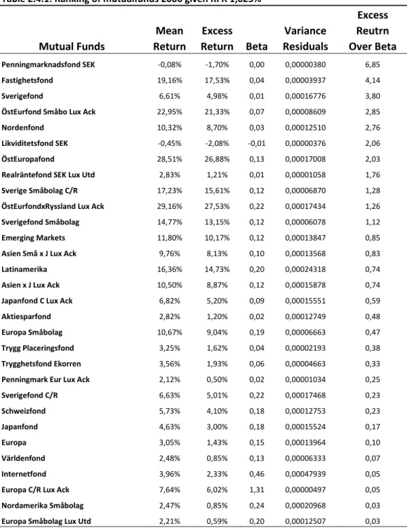
This way we can rank securities before calculation of Cut-off Rate C*. The highest value of C* denote the rate that marks number of securities to be included in the optimized portfolio. optimization process. In my case I am only interested in six mutual funds to invest in so my Cut-off Rate is the same as the sixth security C* value. This because recommended portfolios by SEB Investment Strategy always consist of maximum six investments which is also number of mutual funds that bank clients can invest in via monthly payments. Let us have a look at an example based on values found when applying Vasicek´s technique. Mutual funds in table below are ranked from highest to lowest value of excess return over Beta given
3
Edwin J. Elton/Martin J. Gruber/Stephen J. Brown/William N. Goetzman, Modern Portfolio Theory and Investment Analysis, Sixth Edition, pp 184-189.
historical data 2002-2005 and risk free rate equal to 1,625%4. Notice that for simplicity only 30 out 40 mutual funds are included in the table.
Table 2.4.1: Ranking of mutualfunds 2006 given RFR 1,625%
Excess
Mean Excess Variance Reutrn
Mutual Funds Return Return Beta Residuals Over Beta
Penningmarknadsfond SEK -0,08% -1,70% 0,00 0,00000380 6,85
Fastighetsfond 19,16% 17,53% 0,04 0,00003937 4,14
Sverigefond 6,61% 4,98% 0,01 0,00016776 3,80
ÖstEurfond Småbo Lux Ack 22,95% 21,33% 0,07 0,00008609 2,85
Nordenfond 10,32% 8,70% 0,03 0,00012510 2,76
Likviditetsfond SEK -0,45% -2,08% -0,01 0,00000376 2,06
ÖstEuropafond 28,51% 26,88% 0,13 0,00017008 2,03
Realräntefond SEK Lux Utd 2,83% 1,21% 0,01 0,00001058 1,76
Sverige Småbolag C/R 17,23% 15,61% 0,12 0,00006870 1,28
ÖstEurfondxRyssland Lux Ack 29,16% 27,53% 0,22 0,00017434 1,26
Sverigefond Småbolag 14,77% 13,15% 0,12 0,00006078 1,12
Emerging Markets 11,80% 10,17% 0,12 0,00013847 0,85
Asien Små x J Lux Ack 9,76% 8,13% 0,10 0,00013568 0,83
Latinamerika 16,36% 14,73% 0,20 0,00024318 0,74
Asien x J Lux Ack 10,50% 8,87% 0,12 0,00015878 0,74
Japanfond C Lux Ack 6,82% 5,20% 0,09 0,00015551 0,59
Aktiesparfond 2,82% 1,20% 0,02 0,00012749 0,48
Europa Småbolag 10,67% 9,04% 0,19 0,00006663 0,47
Trygg Placeringsfond 3,25% 1,62% 0,04 0,00002193 0,38
Trygghetsfond Ekorren 3,56% 1,93% 0,06 0,00004663 0,33
Penningmark Eur Lux Ack 2,12% 0,50% 0,02 0,00001034 0,25
Sverigefond C/R 6,63% 5,01% 0,22 0,00017468 0,23 Schweizfond 5,73% 4,10% 0,18 0,00012753 0,23 Japanfond 4,63% 3,00% 0,18 0,00015524 0,17 Europa 3,05% 1,43% 0,15 0,00013964 0,10 Världenfond 2,48% 0,85% 0,13 0,00006333 0,07 Internetfond 3,96% 2,33% 0,46 0,00047939 0,05
Europa C/R Lux Ack 7,64% 6,02% 1,31 0,00000497 0,05
Nordamerika Småbolag 2,47% 0,85% 0,24 0,00020968 0,03
Europa Småbolag Lux Utd 2,21% 0,59% 0,20 0,00012507 0,03
Now, the question is how many of the top ranked mutual funds that are needed in the optimized portfolio. In following table I have calculated the Cut-off Rate for top 30 ranked mutual funds. From table you can see that the value of Ci increases until it reaches the highest
value 0,1476 for Japanfond. Therefore the Cut-off Rate C* is equal to 0,1476 and denotes that
all of the funds up to Japanfond are going to be included in the optimized portfolio given RFR 1,625% and Market variance 0,00007481.
Table 2.4.2: Calculations for Determining Cut-off Rate with Market Variance = 0,00007481
Mutual Funds
Penningmarknadsfond SEK 11 2 11 2 0,0008
Fastighetsfond 189 46 200 47 0,0149
Sverigefond 4 1 204 48 0,0152
ÖstEurfond Småbo Lux Ack 185 65 389 113 0,0288
Nordenfond 22 8 411 121 0,0305
Likviditetsfond SEK 56 27 467 148 0,0345
ÖstEuropafond 209 103 676 251 0,0496
Realräntefond SEK Lux Utd 8 4 683 255 0,0502
Sverige Småbolag C/R 277 216 960 472 0,0694
ÖstEurfondxRyssland Lux Ack 344 272 1305 744 0,0924
Sverigefond Småbolag 253 225 1557 969 0,1086
Emerging Markets 88 103 1645 1071 0,1139
Asien Små x J Lux Ack 59 71 1704 1142 0,1174
Latinamerika 120 161 1824 1304 0,1243
Asien x J Lux Ack 67 91 1891 1395 0,1281
Japanfond C Lux Ack 29 50 1920 1445 0,1297
Aktiesparfond 2 5 1923 1450 0,1298
Europa Småbolag 263 563 2186 2012 0,1421
Trygg Placeringsfond 32 85 2218 2098 0,1434
Trygghetsfond Ekorren 24 75 2242 2172 0,1443
Penningmark Eur Lux Ack 10 39 2252 2212 0,1445
Sverigefond C/R 63 275 2314 2487 0,1460 Schweizfond 58 257 2373 2744 0,1473 Japanfond 34 200 2407 2944 0,1476 Europa 15 161 2422 3104 0,1470 Världenfond 17 258 2439 3362 0,1458 Internetfond 23 446 2462 3808 0,1433
Europa C/R Lux Ack 15845 344744 18307 348552 0,0506
Nordamerika Småbolag 10 282 18317 348835 0,0506
Europa Småbolag Lux Utd 9 322 18326 349157 0,0506
i
Before calculating for weights to be invested in each mutual fund let us have a look at formula for Cut-off Rate.
Recall that stocks are ranked by excess return over Beta (Risk) from highest to lowest. For a portfolio of i mutual funds Ci is given by
N i ei i M N i ei i F i M i R R C 1 2 2 2 1 2 1 2 1 ) ( (2.4.1)Now let us calculate some of Cut-off Rate values. We can start by calculating Ci for top
ranked mutual fund Penningmarknadsfond SEK. That is,
0008 , 0 00014962 , 1 00082291 , 0 2 * 00007481 , 0 1 11 * 00007481 , 0 EK knadsfondS Penningmar C
and for second mutual fund gives
0149 , 0 00351607 , 1 014962 , 0 47 * 00007481 , 0 1 200 * 00007481 , 0 fond Fastighets C
Proceeding in the same fashion we can find all the Ci`s.
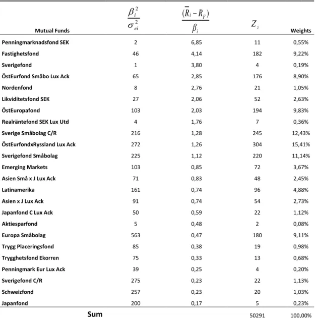
Before calculating for weights to be invested in each mutual fund we know that the final solution will contain 24 mutual funds. That is, all the funds up to Japanfond and the percent invested in fund is
24 1 i i i i Z Z w where * 2 C R R Zi i i F (2.4.2)Applying above equations gives following weights for all mutual funds included in the portfolio.
Table 2.4.3: Calculations for Determining percentage invested in mutual funds up to C*
Mutual Funds Weights
Penningmarknadsfond SEK 2 6,85 11 0,55%
Fastighetsfond 46 4,14 182 9,22%
Sverigefond 1 3,80 4 0,19%
ÖstEurfond Småbo Lux Ack 65 2,85 176 8,90%
Nordenfond 8 2,76 21 1,05%
Likviditetsfond SEK 27 2,06 52 2,63%
ÖstEuropafond 103 2,03 194 9,83%
Realräntefond SEK Lux Utd 4 1,76 7 0,36%
Sverige Småbolag C/R 216 1,28 245 12,43%
ÖstEurfondxRyssland Lux Ack 272 1,26 304 15,41%
Sverigefond Småbolag 225 1,12 220 11,14%
Emerging Markets 103 0,85 72 3,67%
Asien Små x J Lux Ack 71 0,83 48 2,45%
Latinamerika 161 0,74 96 4,88%
Asien x J Lux Ack 91 0,74 54 2,73%
Japanfond C Lux Ack 50 0,59 22 1,12%
Aktiesparfond 5 0,48 2 0,08%
Europa Småbolag 563 0,47 180 9,11%
Trygg Placeringsfond 85 0,38 19 0,98%
Trygghetsfond Ekorren 75 0,33 13 0,68%
Penningmark Eur Lux Ack 39 0,25 4 0,20%
Sverigefond C/R 275 0,23 22 1,13%
Schweizfond 257 0,23 20 1,03%
Japanfond 200 0,17 5 0,23%
Sum 50291 100,00%
Above mix of mutual funds would be one of the portfolios to be compared with SEB Investment Strategy recommended portfolio if number of funds in portfolio where not limited to six. As you will see later in next chapter I will assume that Cut-off Rate C* is always the highest value of Ci among top six ranked mutual funds.
Now that we have covered the theoretical knowledge needed for understanding the steps taken for my study I will in next chapter step by step explain and show how I been using all previous sections in order to answer questions in problem statement.
2 2 ei i i F i
R
R
)
(
3. Method
3.1 Mutual Funds
SEB's fund range consists of approximately 150 funds, all not taken into account in this study because the majority of them did not meet the criterias I have set. They are:
1. Clients must be able to invest in funds through conventional SEB Fund Account.
2. No initiation fees or sales charges.
3. Minimum historical Net Asset Value prices (NAV-prices) from 2nd January 2002.
4. Daily trading and at least 300 million SEK in assets under management. 5. No Fund-in-Fund products.
6. Only SEB or SEB Choice funds.
Criteria 1 to insure that future allocation is possible for SEB Retail clients since some of mutual funds are only available to SEB Private Banking clients and some only possible to invest in via insurance policies. Criteria 2 because fees for entry or exit complicates calculation of expected yield and limits the possibility for re-allocations. Criteria 3 to insuring that data is not dependent on only one kind of market behavior. First January 2002 was decided to be the starting point because it was the earliest date that most mutual funds had historic data from. Criteria 4 so that mutual fund´s share of Index could have a significant impact on the market portfolio. Criteria 5 since fund-in-fund products can most possibly contain funds already included in Index. Criteria 6 because external fund´s asset under management are not only based on inflow from SEB´s clients and their magnitude can therefore have to much impact on Index.
Due to criteria Index consisted of 40 mutual funds between 2002-01-01 to 2007-12-31 and 37 between 2008-01-01 to 2009-12-31. All funds along with their asset under management 2005 to 2008 are shown in Appendix I.
Mutual funds Fastighetsfond, Asien Små x J Lux Ack and Europa Småbolag Lux Utd had all less then 300 MSEK in assets when measured January 2008 and therefore excluded from index measurement 2008 and 2009.
3.2 Purpose
Before we move on to optimisation steps let us repeat what I want to achieve with this work. The objective is to evaluate the investment recommendations SEB Investment Strategy has proposed January 2006 to December 2009. Evaluation could be done by comparing the yield on the above measurement period with the return of an index, for example OMX30 or the MSCI World Net Return Index. But then the evaluation would stop at only one assessment by comparison. What I instead want to achieve is to evaluate by comparing with other portfolios generated by applying the Vasicek's Technique. This way I can demonstrate if the portfolio allocation technique results in better investments than the proposals given by SEB Investment Strategy between the years 2006 - 2009, these proposals are summarized in Appendix II. During those four years new portfolios were recommended on twelve occasions, which means that at each moment, four different compositions were recommended, FP30, FP50, FP70 and FP100. Each portfolio tailored to the investor's willingness to take risks and expected return. For each portfolio, I will develop an optimized solution using Vasicek's Technique and the simplified optimization process. This will be done on four occasions, the first four optimized portfolios OP1, OP2, OP3 and OP4 are produced in January 2006, their composition remains unchanged throughout 2006 and the process will be repeated again in January 2007, 2008 and 2009. For each year one year historical data will be added to the measurements which form the basis for the optimization process. The idea is to compare OP1 with FP30, FP50 with OP2, OP3 with FP70 and finally OP4 with FP100. But how will I be able to produce comparable portfolios? For example, I can measure the risk of FP30 and optimize the return given that risk, and repeat the process for FP50, FP70 and FP100. That way I can take up four optimized portfolios that initially have the same risk as recommend portfolios where returns have been maximized. Unfortunately, the results may not only consist of up to six funds, which is the requirement for the portfolios if they will be fairly comparable with recommended portfolios. If I instead choose to measure the return and minimize risk given that return in the optimization process, occurs first the problem with a maximum of six funds,
and also problems with negative returns in some measurement periods. It is because of this that I have chosen to apply the simplified optimization process where I can pre-determine the number of funds in the portfolio by assuming that C* is equal to the highest of the six highest ranked portfolios Cut-off Rate and by changing risk-free rate we can create four different portfolios with different risk levels. How this is done we will return to later in this chapter when I describe how portfolios are developed. The risk-free interest rate will play another important role in the optimization process. At each optimization process, I will bring the risk-free interest rate equal to the actual interest rate on a SSVX1M. The portfolio to be developed with respect to this interest is then compared with FP100, which only consists of equity funds. The reason for this is that I assumed that, if an investor has the opportunity to invest in the risk-free rate but chose another option than he is interested in a portfolio with the largest proportion of equity funds. The other three portfolios are optimized given risk-free rate plus 2% premium each time. Higher risk-free interest rate contributes to lower risk in the portfolio when the model is weighted more to assets with less risk, which usually happens to be fixed-income funds. By letting the risk-free interest rate to be determined by actual interest rate on a 30 day treasury bill contributes to other benefits. If interest rates are low, the model will automatically be folded more in equity funds for all portfolios since the base to which premiums are added will be lower and vice versa when the risk-free interest rate is higher.
3.3 Market Portfolio (Index)
As explained in Chapter 2 section 2.4 we need to find out values for forecasted Alpha, Beta, variance of residuals, market return and market variance to be able to conduct the optimization process. So first of all we need a market portfolio (Index) to which we can relate mutual funds return and risk. Recall that from January 2002 to December 2007, 40 mutual funds passed the criteria’s and therefore were available to invest in when first optimization process started January 2006. A list of all these funds can be seen in Appendix I along with wealth under management from 2005 to 2008. Daily time series for each of these funds where downloaded from seb.se/fonder from January 2002 to December 2009 except for three funds whose wealth decreased under 300 MSEK when measured January 2008. These three funds Fastighetsfond, Asien Små x J Lux Ack and Europa Småbolag Lux Utd where therefore excluded from Index during last historical period 2008. Thus Index consisted of 40 funds
from beginning of 2002 to end of 2007. For the first optimization process January 2006 each fund´s assets as of January 2005 where divided by total assets under management (AUM) at the same time in order to find out it´s share of Market portfolio. These proportions were then multiplied to their own prices, then added together for each day to sum up daily time series of market portfolio (Index). So if each year consists of 250 time series and we need to find out dayli time series for Index from January 2002 to December 2005 then
40 1 i ij i Mj X P P j = 1, … , 1000 days 1 MP first day NAV-price of Index
1 i
P first day NAV-price of mutual fund i
2005 2005 total i i AUM AUM X
For each subsequent year after 2005 new proportions where calculated by updating AUM for mutual funds and divide by total AUM given by volumes in columns of Table in Appendix I. Given share of Index the procedure where repeaded and dayli time series for market portfolio where obtained for whole period January 2002 to December 2008. Given these prices I could move forward to obtain historical values according to steps in theory section about SIM.
3.4 Obtaining Historical Variables
Recal from Chapter 2.4 Simplified Technique for Finding Optimal Portfolios, that mutual funds where ranked with respect to excess return over Beta, that is
i F i R R where M i i i R R i
is the component of mutual fund i´s return that is independent of the market´s performance.
i
a constant that measures the expected change in Ri given a change in RM
and also a measure of risk. RF = Risk free rate
M
R Expected return of the market portfolio
All variables except for the risk free rate are based on historical estimates, but since Vasicek´s Technique is the method applied in this work we are interested in forecasted values for Alpha and Beta instead of their historical estimates. Therefore both Alpha and Beta are replaced by their forecasted estimates
1 1 i F i R R where M i i i R R1 1 1 i i i 1 0,5 0,5 i
average Alpha estimated from periodic data
i i i i i i i i i 2 2 2 2 2 2 1 i
average Beta estimated from periodic data
2 2 2 M ei i 2 ei variance of residuals 2 M
variance of market portfolio
T j i itj T 1 2 2 1 1 itj sub period tj Beta
From above summary we see that forecasted estimates of Alpha and Beta are dependent on their historical and average estimates. In the text that follows I will only describe the methods used for measurement of historical data.
Historical Alpha, Beta and Variance of Residulas
The reason for grouping above three variables is that all three can be calculated by the use of Excel Regression analysis tool-pak. Where you choose daily average return of mutual fund as Input Y Range and daily average return of market portfolio as Input X Range. Then, by pressing OK a new Worksheet is produced showing historical Alpha as Intercept, Beta as X Variable and variance of residuals in Residula row and MS column as shown below for one of the mutual funds
Expected Return and Variance of Market Portfolio
Average return of market portfolio is simply calculated by the use of Excel command =AVERAGE(number1;[number2];…) where numbers inside brackets are the daily return data for the historical period under consideration. Annualised expected return can instead be measured by summing up daily returns for the historical period needed. Note that this command calculates the arithmetic mean of arguments inside brackets. I choosed arithmetic mean instead of geometric because the latter only applies to positive numbers whereas data analysed also contain negative numbers.
Market variance is measured following same steps as above and command VARP which measures variance with respect to entire population.
All historical estimates for periods previous to forecast year are summarized in Appendix III, Table 1.
3.5 Obtaining Forecasted Variables
Each historical period was divided into sub periods each containing six month daily data of return. For examble, the first historical period ranging from January 2002 to December 2005 contained eight sub periods. For each sub period average return of market and mutual funds, variance of market, and covariance between Index and mutual funds where computed for calculation of each sub period Alpha and Beta. The computation resulted in eight Alpha and Beta values. Taking average of these values with Excel command AVERAGE, and VARP of Beta values (2i) we have most of the data needed for computing forecasted Alpha and Beta for year 2006 according to following formulas
i i i 1 0,5 0,5 1 8 8 1
j ij i Mj ij ij ij R R j = 1, … , 8 2 Mj ijMj ij j = 1, … , 8 i i i i i i i i i 2 2 2 2 2 2 1 where 1 8 8 1
j ij i and 2 2 2 M ei i (computed with historical estimates)
All subperiod data alond summary of periods and forecasted values are summarized in Appendix III, Table 2 and 3.
3.6 Optimisation
As explained earlier, optimization ca be done through various ways where I have covered four of them. I could measure the risk value for each recommended portfolio and maximize return given that risk for a solution comparable to those recommended by SEB Investment Strategy. Doing so could result in portfolios consisting of less or more mutual funds then those six suggested by SEB Investment Strategy and therefore not comparable since I should construct portfolios given same constraints.
Measuring return of recommended portfolios and minimizing risk given that return would also result in portfolios with more or less mutual funds then six and as I discovered some periods resulted in negative return which are inappropriate when computing optimized portfolios. This since a riskaverse investor would never in advance knowing that the portfolio he investing in has an expected return which results in losses.
Working with Sharpe-Ratio through maximization of it given different risk-free rates that anables four solutions to compare with recommended portfolios FP30, FP50, FP70 and FP100 could also result in portfolios not consisting of maximum six mutual funds.
Due to these matters I finally decided to apply the simplified optimization technique covered in Chapter 9 of Modern Portfolio Theory and Investment Analysis book5. The technique was then adjusted to make possible maximum six mutual funds to be included in the optimized solution. You may argue that this adjustment may result in portfolios that are not fully optimized since as we have seen the solution without adjustment may result in a portfolio with more than six mutual funds (example on page 14, Table 2.4.3). That may be true but outside the topic of this paper. For my needs I just needed a technique that with which I could predetermine number of mutual funds available to invest in without arbitrary thinking.
My next challenge was to determine a way that enables optimization that results in four solutions with different risk levels. Increasing risk free rate resulted in portfolios that consisted of higher degree interest funds and therefore less risk. But where to start and how much increase? I argued that the lowest risk free rate and therefore the solution with highest
5
Edwin J. Elton/Martin J. Gruber/Stephen J. Brown/William N. Goetzman, Modern Portfolio Theory and Investment Analysis, Sixth Edition pp 183-189.
share of equity funds would equal to actual T-bill at the time for the optimisation process. The argument is that given that rate in the calculation of mutual funds enables the possibility to only invest in the risk free asset but the investor is interested in other investments but increasing the rate may affect investor to adjust to more interest-bearing alternatives. I decided to increase with 2 % each time since lower increase did not have the measurable affect equal to recommended portfolios where share of interest funds increases from 0 % for FP100 to 30 % for FP70, 50 % FP50, and 70 % FP30. An increase more than 2 % resulted in portfolios with to much interest funds and therefore 2 % seemed best suitable to work with.
As you will see in next chapter the portfolios optimized do not consist of equal amount interent funds to those they are compared with, some years they are less and some years they are more, and for the case of FP100 with 100 % equity founds the optimized solution always consists of some degree of interest funds but that does not necessarirly mean that it is less risky as it will be proven in next chapter.
4. Result
4.1 FP100 vs OP1
The first set of portfolios to be compared is FP100 with 100% equity funds recommended in January 2006 and optimized portfolio 1 (OP1) resulted given risk-free rate 1,625% yearly return and historical data years 2002 to 2005. The composition of funds in OP1 will be unchanged throw whole 2006 but FP100 will be reallocated six times according to weights in Appendix II. The comparison will be continued in same manner with new set of optimized portfolios January 2007, 2008 and 2009. We will start by examining each year and finally summarize for whole period January 2006 to December 2009.
FP100 vs OP1 2006
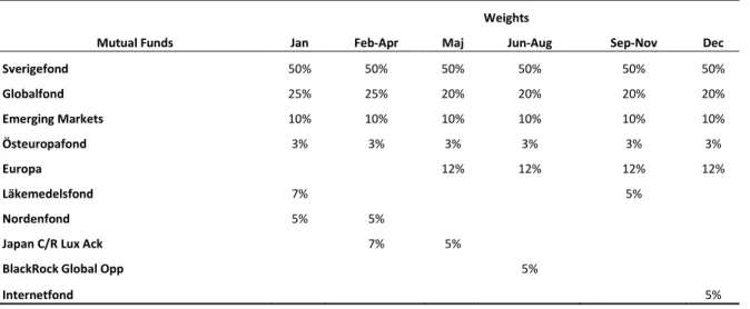
The first 100% equity fund recommended by SEB Investment Strategy (SEB IS) consisted of funds and weights according to first weight column in below table. Funds where replaced and weights updated six times during 2006 which can be followed in same table.
Table 4.1.1: FP100 during 2006
Weights
Mutual Funds Jan Feb-Apr Maj Jun-Aug Sep-Nov Dec
Sverigefond 50% 50% 50% 50% 50% 50% Globalfond 25% 25% 20% 20% 20% 20% Emerging Markets 10% 10% 10% 10% 10% 10% Östeuropafond 3% 3% 3% 3% 3% 3% Europa 12% 12% 12% 12% Läkemedelsfond 7% 5% Nordenfond 5% 5%
Japan C/R Lux Ack 7% 5%
BlackRock Global Opp 5%
Internetfond 5%
By investing in first recommended portfolio and reallocate each day so that allocation always is the same as latest recommended portfolio an investors return was equal to 12,33% during 2006. The optimized alternative shown in below table returned during same period 24,73%.
Table 4.1.2: OP1 January 2006
Adjusted
Mutual Funds Weights Weights Penningmarknadsfond SEK 2,41% 2%
Fastighetsfond 40,54% 40%
Sverigefond 0,84% 1%
ÖstEurfond Småbo Lux Ack 39,64% 40%
Nordenfond 4,68% 5%
Likviditetsfond SEK 11,89% 12%
Summarizing both portfolios below shows that OP1 returned almost dubble the return of FP100 with almost same level of risk. Ranking them with respect to risk and risk-free rate 1,625% shows that optimized solution ratio exceeded recommended portfolios by more than 100%. Note that OP1 contained 14% interest-bearing funds compared to FP100 which contained none.
Table 4.1.3: Summary of data 2006
Portfolio Data FP100 OP1
Return 12,33% 24,73%
Risk 9,88% 10,06%
Sharpe Ratio 1,08 2,30
FP100 vs OP1 2007
During 2007 recommended portfolio was only reallocated two times according to weights in below table with first column wights equal to the weights for December in Table 4.1.1.
Table 4.1.4: FP100 during 2007
Weights
Mutual Funds Jan-Apr May-July Aug-Dec
Sverigefond 50% 50% 50%
Globalfond 20% 20% 20%
Europa 12% 12% 12%
Emerging Markets 10% 10% 10%
Östeuropafond 3% 3%
JPM Global Natural Resources 5% 5%
Internetfond 5%
GS BRIC´s Portfolio 3%
Optimised alternative contained 27% interest funds compared to 14% when optimized during 2006 because of higher risk-free rate which increased to 2,985% January 2007.
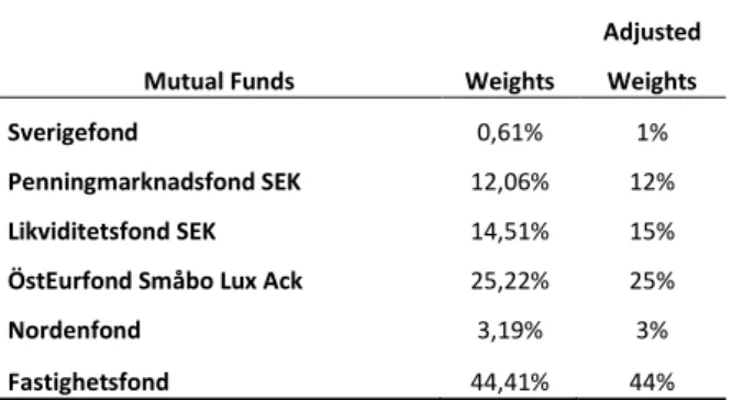
Table 4.1.5: OP1 January 2007
Adjusted
Mutual Funds Weights Weights
Sverigefond 0,61% 1%
Penningmarknadsfond SEK 12,06% 12%
Likviditetsfond SEK 14,51% 15%
ÖstEurfond Småbo Lux Ack 25,22% 25%
Nordenfond 3,19% 3%
Fastighetsfond 44,41% 44%
Despite the high proportion of fixed-income funds OP1 resulted in 13,06% loss during 2007 compared FP100´s 0,09% positive return.
Table 4.1.6: Summary of data 2007
Portfolio Data FP100 OP1
Return 0,09% -13,06%
Risk 12,23% 11,90%
Sharpe Ratio neg neg
FP100 vs OP1 2008
During 2008 recommended portfolio was only reallocated once in September with the first set of portfolio equal to the last one in 2007.
Table 4.1.7: FP100 during 2008
Weights
Mutual Funds Jan-Aug Sep-Dec
Sverigefond 50% 50%
Globalfond 20% 15%
Europa 12% 10%
Emerging Markets 10% 7%
GS BRIC´s Portfolio 3% 3%
JPM Global Natural Resources 5%
Nordamerika C/R Lux Ack 15%
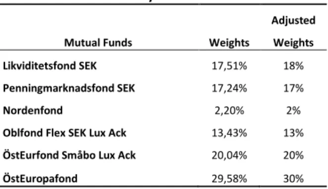
January 2008 a Swedish Government T-bill returned 4,05% which as expected increased the proportion of fixed income funds from 27% for previous year to 48% this year.
Table 4.1.8: OP1 January 2008
Adjusted
Mutual Funds Weights Weights Likviditetsfond SEK 17,51% 18%
Penningmarknadsfond SEK 17,24% 17%
Nordenfond 2,20% 2%
Oblfond Flex SEK Lux Ack 13,43% 13%
ÖstEurfond Småbo Lux Ack 20,04% 20%
ÖstEuropafond 29,58% 30%
Both portfolios crashed during 2008, FP100 with 47,44% and OP1 by 62,27%. Eastern European markets where among hardest-hit markets because of financial crisis. The adjustment to fixed income funds lowered the potential greater loss but still the high degree of
eastern European funds resulted in both higher volatility and greater loss compared to recommended portfolio.
Table 4.1.9: Summary of data 2008
Portfolio Data FP100 OP1
Return -47,44% -62,27%
Risk 16,64% 22,58%
Sharpe Ratio neg neg
FP100 vs OP1 2009
FP100 was reallocated two times during 2009 with first set of portfolio equal to last one in 2008. For the first time since we started the comparison, investments in Swedish equity market decreased from constant 50% to now 20%.
Table 4.1.10: FP100 during 2009
Weights
Mutual Funds Jan-Mar Apr-Sep Oct-Dec
Sverigefond 50% 20% 20%
Globalfond 15% 30% 25%
Nordamerika C/R Lux Ack 15% 15% 15%
Europa 10% 15% 15%
Emerging Markets 7% 10% 15%
JF China Fund 10%
GS BRIC´s Portfolio 3%
Listed Private Equity 10%
Risk-free rate (SSVX1M 2009-01-02) decreased from 4,05% to 1,6% from January 2008 to January 2009. The 2,45% decrease resulted in 29% less investments in fixed-income funds compared to 2008. One may argue that even Penningmark Eur Lux Ack is a interest-bearing fund. That is true, but for a Swedish investor it is more likely to be considered as a FX fund in Euro.
Table 4.1.11: OP1 January 2009
Adjusted
Mutual Funds Weights Weights Likviditetsfond SEK 9,25% 9%
Penningmarknadsfond SEK 8,22% 8%
Penningmark Eur Lux Ack 16,81% 17%
ÖstEuropafond 23,70% 24%
Realräntefond SEK Lux Utd 2,18% 2%
ÖstEurfondxRyssland Lux Ack 39,84% 40%
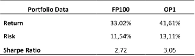
Summary shows that both portfolios returned positive with almost same level of risk. OP1 increased by 41,61% which was 8,59% higher then FP100. With only 1,57% more risk which resulted in higher Sharpe-ratio.
Table 4.1.12: Summary of data 2009
Portfolio Data FP100 OP1
Return 33.02% 41,61%
Risk 11,54% 13,11%
Sharpe Ratio 2,72 3,05
FP100 vs OP1 2006 – 2009
By daily reallocation and with portfolios that reflected the last recommended or optimized portfolio an investor where slightly better of following SEB Investment Strategy´s suggestions. FP100 decreased by 2% whereas OP1 resulted in 8,99% loss. OP1 was 2,47% riskier. Data summarized in following table and graf.
Table 4.1.13: Summary of data 2006-2009
Portfolio Data FP100 OP1
Return -2,00% -8,99% Risk 12,96% 15,43% -0,6 -0,4 -0,2 0 0,2 0,4 0,6 FP100 OP1
4.2 FP70 vs OP2
This time we are going to compare recommended portfolio with 30% fixed level of interest-bearing funds with OP2 optimized in the same manner as OP1 but with 2% added to actual risk-free rate at the time for optimization process.
FP70 vs OP2 2006
Six portfolios was recommended by SEB IS during 2006. Oblfond Flex SEK Lux Ack was the fixed income fund choosed as a way to lower the risk in the portfolio for making it suitable to investors with shorter investment horizon or more reluctant to risk.
Table 4.2.1: FP70 during 2006
Weights
Mutual Funds Jan Feb-Apr Maj Jun-Aug Sep-Nov Dec
Oblfond Flex SEK Lux Ack 30% 30% 30% 30% 30% 30%
Sverigefond 35% 35% 35% 35% 35% 35% Globalfond 19% 19% 15% 15% 15% 15% Emerging Markets 7% 7% 7% 7% 7% 7% Europa 9% 9% 9% 9% Läkemedelsfond 5% 4% Nordenfond 4% 4%
Japan C/R Lux Ack 5% 4%
BlackRock Global Opp 4%
Internetfond 4%
The optimized alternative given RFR 1,625% + 2% contained nearly same degree of fixed-income to equity funds 28/72 compared to above portfolios which contained 30/70. Same mutual funds as OP1 during 2006 where ranked among top six with only difference being the portion invested in them.
Table 4.2.2: OP2 January 2006
Adjusted
Mutual Funds Weights Weights Penningmarknadsfond SEK 5,02% 5%
Likviditetsfond SEK 22,48% 23%
Fastighetsfond 34,30% 34%
ÖstEurfond Småbo Lux Ack 34,29% 34%
Sverigefond 0,48% 1%
FP70 returned 6,44% while OP2 23,48% which is 17,04% more then recommended portfolio. On the contrary OP2´s return where more volatile during 2006 and the risk exceeded FP70´s by 3,92% but since the gain of that risk was better then portfolio being compared to its Sharpe-ratio was 168% higher
Table 4.2.3: Summary of data 2006
Portfolio Data FP70 OP2
Return 6,44% 23,48%
Risk 5,65% 9,57%
Sharpe Ratio 0,85 2,28
FP70 vs OP2 2007
FP70 was only reallocated once during 2007 by replacing Internetfond with JPM Global Natural Resources with the first set of portfolio equal to last one in 2006. The optimized alternative OP2 contained 49% fixed income funds due to higher RFR compared to 2006. But still this portfolio resulted in 11.10% loss compared to 3,61% gain for the recommended portfolio. Its risk level was also higher then FP70´s by 3,55%. Tables on next page shows what is been mentioned.
Table 4.2.4: FP70 during 2007
Weights
Mutual Funds Jan-Apr May-Dec Oblfond Flex SEK Lux Ack 30% 30%
Sverigefond 35% 35%
Globalfond 15% 15%
Europa 9% 9%
Emerging Markets 7% 7%
JPM Global Natural Resources 4%
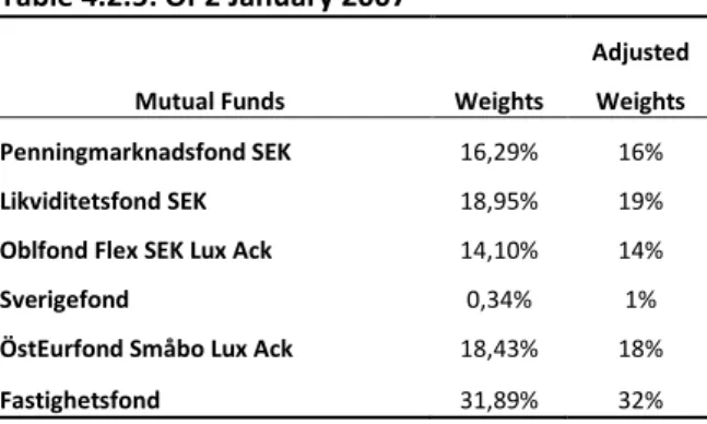
Table 4.2.5: OP2 January 2007
Adjusted
Mutual Funds Weights Weights Penningmarknadsfond SEK 16,29% 16%
Likviditetsfond SEK 18,95% 19%
Oblfond Flex SEK Lux Ack 14,10% 14%
Sverigefond 0,34% 1%
ÖstEurfond Småbo Lux Ack 18,43% 18%
Fastighetsfond 31,89% 32%
Table 4.2.6: Summary of data 2007
Portfolio Data FP70 OP2
Return 3,61% -11,10%
Risk 6,85% 10,40%
Sharpe Ratio 0,09 neg
FP70 vs OP2 2008
FP70 was only reallocated once in September 2008 with small changes. OP2 contained 68% fixed-income funds but it did not help much and both potfolios crashed as expected, FP 70 by 23,29% and OP2 by 39,08%. One would expect that the high degree of low risk funds in OP2 should result in less risk but supricingly volatility of OP2 exceeded FP70 by 5,41%. Once againg investments in eastern European funds resulted in greater loss and higher volatility. All data summarized in following three tables.
Table 4.2.7: FP70 during 2008
Weights
Mutual Funds Jan-Aug Sep-Dec Oblfond Flex SEK Lux Ack 30% 30%
Sverigefond 35% 35%
Globalfond 15% 10%
Europa 9% 8%
Emerging Markets 7% 7%
Nordamerika C/R Lux Ack 10%
Table 4.2.8: OP2 January 2008
Adjusted
Mutual Funds Weights Weights Likviditetsfond SEK 18,34% 18%
Penningmarknadsfond SEK 18,45% 19%
Oblfond Flex SEK Lux Ack 31,01% 31%
Nordenfond 1,07% 1%
ÖstEuropafond 19,00% 19%
ÖstEurfond Småbo Lux Ack 12,13% 12%
Table 4.2.9: Summary of data 2008
Portfolio Data FP70 OP2
Return -23,29% -39,08%
Risk 9,09% 14,50%
Sharpe Ratio neg neg
FP70 vs OP2 2009
FP70 was reallocated once in April 2009, only this time with not small changes. After big losses in almost every recommended portfolios the pressure increased to abandon the old strategy. This time the weights invested in Oblfond Flex SEK Lux Ack decreased from 30% to 20%, the large proportion invested in Sverigefond also decreased from 30% to 15%. Asset Selection the best fund in 2008 and very popular were picked in. But question remains if this change of strategy came to late.
Table 4.2.10: FP70 during 2009
Weights
Mutual Funds Jan-Mar Apr-Dec Oblfond Flex SEK Lux Ack 30% 20%
Sverigefond 35% 15%
Globalfond 10% 25%
Nordamerika C/R Lux Ack 10% 15%
Emerging Markets 7% 10%
Asset Selection 15%
Europa 8%
The optimized portfolio still very heavy invested in high risk markets did well during high yielding year of 2009. OP2 return equaled 39,49% which was 31,6% higher then FP70. As prior cases the volatility remained higher even this year and exceeded FP70´s risk by 4,85%.
Table 4.2.11: OP2 January 2009
Adjusted
Mutual Funds Weights Weights Likviditetsfond SEK 17,13% 17%
Penningmarknadsfond SEK 16,36% 16%
ÖstEuropafond 14,90% 15%
Oblfond Flex SEK Lux Ack 3,92% 4%
ÖstEurfondxRyssland Lux Ack 23,96% 24%
Latinamerika 23,73% 24%
Table 4.2.12: Summary of data 2009
Portfolio Data FP70 OP2
Return 7,89% 39,49%
Risk 6,14% 10,99%
Sharpe Ratio 1,02 3,45
FP70 vs OP2 2006 – 2009
Summarising data shows that an investor where better of investing in OP2 but you must note that this portfolio´s risk were 4,57% higher then portfolio recommended by SEB IS.
Table 4.2.13: Summary of data 2006-2009
Portfolio Data FP70 OP2
Return -5,34% 12,79% Risk 7,11% 11,68% -0,4 -0,3 -0,2 -0,1 0 0,1 0,2 0,3 0,4 0,5 FP70 OP2