Formation of House Prices in Sweden

I

H

HÖGSKOLAN I JÖNKÖPING

Formation of House Prices in

Sweden

Master Thesis in Economics

Authors: Gabriel Cardona Cervantes

Tutors: Lars Pettersson

Marie Lidbom

Date: 2009-09-11

Jönköping

Master Thesis in Economics

Title: Formation of House Prices in Sweden

Authors: Gabriel Cardona Cervantes 870307-0030

Tutors: Lars Petterson

Marie Lidbom

Date: 2009-09-10

Keywords: Swedish financial crisis, Regional house prices, Asset and Property

price estimations, Regional differences in housing markets.

JEL codes: R21, R31, R38, G01, G11, E31, E32

Abstract

In this research, Sweden’s municipalities are categorized into five economic regions which put emphasis on location. Furthermore, since house prices reflect and are reflected by the existing cycles in the economy, four time periods are considered. By using extensive data collected by Sweden Statistics (SCB), this study tests eight variables factors to be used in a cross-section analysis which will help researchers understand which factors are consistent in explaining the formation of house prices in terms of location and time. The conclusion that can be drawn is that no factor can fully explain house prices at a national level and that the Population variable was consistent in regional changes and Employment was consistent in time changes. This has lead to a greater understanding of the field of regional house prices in order for it to contribute to real estate investments or purchases.

Introduction...4

Purpose...4

Outline...4

Financial Crisis in Sweden during the 1990s...5

Deregulations of the credit and exchange system...6

Tax reforms...6

Other reforms...6

The post 1990s crisis...7

Previous Studies ...8

Theory ...10

Data and Methodology...15

Regional Division...17

Regression Model...19

Hypotheses ...19

Results & Analysis...20

Conclusions...26

Suggestions for Further Research...27

References ...28

Tables

Table 1 - Variables and suggested signs...16

Table 2 - Regression Results 1991-1994...20

Table 3 - Regression Results 1995-2000...22

Table 4 - Regression Results 2000-2003...23

Table 5 - Regression Results 2003-2007...24

Table 6 - Details of regional division...30

Figures Figure 1 - House Price Dynamics...11

Figure 2 - The Rent Gradient Law...13

Figure 3 - Portfolio investment...15

Figure 4 - Regional divisions in Sweden...18

Equation Equation 1 - Hedonic Price General...12

Equation 2 - Hedonic Price Definition...12

Equation 3 - Hedonic Price Regional...12

Introduction

The value of every real estate stands for the largest single component of national wealth and is one of the most important assets for a household during their life time. To estimate the annual value for real estate, the investment of GDP for construction and building materials is partly takes into account. However, when estimating the actual space used by real estate, its value should be counted as stock or wealth, since land is a national asset (Wheaton & DiPasquale, 1996). The subject about real estate prices is an interesting theme for households, national economists and investors. Its unique characteristics allow not only for space to be lived in, but helps to explain certain interactions with the national economy and can be the subject of potential investments. Thus, from a household perspective, it is not only about finding a place of its own, it is also of household interest to know where and when to buy a house for investment purposes. This also leads to a national interest which can be reflected on the previous economic crisis in Sweden. Between the years 1991-1993, Sweden suffered from industrial sector crisis, macroeconomic imbalances and major economical and political uncertainties. The Swedish GDP fell continuously and at its worst, state debt peaked at 85% of GDP (Hultkrantz & Söderström, 2009). Sweden is regionally divided in 290 municipalities located within 21 regions. Like in many countries, the regions are differently categorized in density of population and economic activity. Therefore, the regions are also divided into 72 of the most economically important regions. For instance, the Stockholm region is the most economically active region in the country, followed by the Gothenburg and Malmö regions. The less populated regions differ not only in its economic size but also in its regional characteristics at a non-national level in different time periods. Therefore, instead of the conventional macro-theory in economics were everything is measured at a national level, one should emphasize the importance of economics at a regional level and its changes over time. Here, this type of economics is devoted to house prices in four different cycle periods and in five different regional groups. So, the important question when dealing with house prices is: Which determining factors are consistent between regions and time and which are consistent for the whole country?

Purpose

The purpose of this thesis is to find out what factors or variables form house prices between regions and between different time periods. The study identifies variables that are national, location-specific and time-specific and define their characteristics. The variables are of regional importance and are the following: population, employment, income, interest cost, house stock, sold houses, internal and external migration. This will give value to certain factors that form house prices and present its interregional complexities.

Outline

The background section will present the most important changes in the Swedish house market from the beginning of the 1990s to understand the specific case of Sweden. The third section will present the Swedish case in relation to previous studies of regional house prices and its effects on other countries. The fourth section contains information about fundamental theories regarding the dynamics and diversities of house prices. With the theories from the previous sections, the fifth section presents the data that will be used for empirical testing. The sixth section shows the empirical results and analyzes its implications on regional house prices. Lastly the seventh section concludes the study in a brief and succinct manner.

Financial Crisis in Sweden during the 1990s

The history of the economic development in the Swedish welfare system is an informative way of understanding the recent developments in the Swedish house market. Even though this thesis is primarily concentrated on empirical findings at the regional level, one must also consider the important aggregate effects of the whole Swedish economy. The fact that Sweden came into a crisis was due to a series of new institutional developments that caused house prices to inflate based on massive speculation. By the end of the 1980s, the underlying problems from low productivity, higher nominal salaries, household debt and rigid labour market showed its true colours during the 1990-crisis.

In 1970, Sweden was the 4th _{richest nation in the world. But along the 1970s the golden}

years of the Swedish economy started to deteriorate. Since then, an unpredictable government undermined the private ownership rights by imposing tax rates and regulations each year. Furthermore, up until 1992, Sweden was under a fixed exchange rate regime and underwent constant devaluations that helped foster their export industry and spur inflation. Devaluations of the Swedish Krona were constantly fluctuating which led to currency speculations and difficulties of long-term planning. Furthermore, Sweden experienced limited freedom of trade, regulated capital markets and inefficient allocation of productive resources (Bergh, 2007). In addition, the government implemented vast numbers of subsidies for industries facing economical problems since Sweden did not tolerate high differences in income between sectors. This gave a vague impression of which businesses where blooming and which were failing. Due to state controls and subsidies, the industries lost productivity and employers faced problems with their employment cost containing high taxes, tight regulations and higher nominal wages (Bergh, 2007). This led to the recession in the 1990s which was further exacerbated by the oil war between Iraq and Kuwait. The industry had to make cuts in all sectors which in turn affected the commercial real estate industry. The construction sector diminished which then affected the financial institutions and the banks. Sweden was left with a bad state finance and unemployment, so the Swedish economy lost credibility. This made it impossible to sustain the fixed exchange rate regime. The reaction to constant devaluations was stopped by tying the Krona to the Euro and the Swedish Krona lost 20% of its value. The new order was changed to floating exchange rates and a monetary policy focused on keeping inflation between 1-3% compared to having inflation above 10% for a long time (Reeman, Swedenborg, Topel, 2006).

In the 1980s a lot of reforms and deregulations were made that changed the economy into a more globalized market economy. In addition, other changes that were already implemented before the 1980s also came into effect in the early years of the 1990s (Berg, 2007). When joining the EU, Sweden regained its financial credibility in the latter half of the 1990s. This strengthened the Swedish Krona and reduced the interest rate. However, despite the lower inflation the unemployment did not fall until much later (Giertz, 2008). In retrospect, the general problems were the needs to reduce unemployment, budget deficit and the needs to achieve stable and long-term economic expansion. Cuts in the public sector were greater when low productivity industries where privatized.

Deregulations of the credit and exchange system

In 1974, the Swedish Central Bank had a strict credit system towards lending to commercial banks and primarily financed the public sector. The existing law was in vigour

between 1939 and 1974 which restricted the in and out flow of capital. In 1985 the rules were considered inefficient and the abolishment was made in 1989. Between those years, the credit system was then gradually abolished for three reasons: the rules became less important, they had lost efficiency and there was too much biasness in credit allowance. Since 1993, the Riksbank was keen on making itself independent from the ruling government at the time. From 1993, monetary policy would aim at preventing the increase in the underlying rate of inflation (Bergh, 2007).

Tax reforms

Between the years 1977-1982 households with higher incomes had tax rates around 85-88%. In addition, when adding the payroll tax, wealth tax and the marginal tax, rates could sometimes exceed 100%. At one occasion in 1980s and another in the 1990-1991 period, two great tax reforms, decreased progressive taxes and imposed indirect taxes such as duty taxes on purchased items. Sweden then went from highly progressive taxes to milder and proportionate ones throughout the whole taxpaying population. Due to the fact that interest costs were tax-deductible, the constant inflation lowered the borrowing cost and with the new abolishment of the credit regulations, it caused a major boom in household lending, especially in the real estate market. Changes in the house prices affects the capacity to borrow (collateral effect) while movements in consumer prices (inflation) influence the real value of that debt (debt deflation). Thus, a positive demand shock results from increases in house prices which raises the capacity to borrow, thereby further stimulating demand. The increase in consumer prices transfers wealth from lenders to borrowers. With borrowers higher propensity to consume, this raises aggregate demand even further (Finocchiaro, 2007). But with new changes in taxes, borrowing cost increased and inflation fell which encouraged savings. This is when the demand for housing shrunk and the 1990 crisis in Sweden started. Berg (2007) also examines the timing of the new deregulations. For instance, had the tax reform succeeded before the credit de-regulation the crisis might not had given such an impact. However, as many countries went through a similar process of deregulation which led to similar results elsewhere; it might have been an inevitable process.

Other reforms

Apart from the most important deregulations, changes to new establishments played an important role to reform of the Swedish structure: in 1992, municipalities were given greater autonomy through decentralization to organize fields such as schools, health care and the labour market policy. In 1995, Sweden joined the EU came into benefiting the four freedoms of mobility. A new budget process was made were forecast and transparency in the market is set with respect to current cyclical movements. Agriculture policies were implemented to fight domestic problems which enacted agriculture subsidies. Social insurance reform and retirement reform were also implemented (Berg, 2007). Despite the reforms, Sweden still remains a welfare state and has not departed into an extreme market economy. However, since the 1990s crisis, Sweden has increased its economic freedom perspective and has been widely influenced by globalization and liberalization.

The post 1990s crisis

Between the late 1990s and the early 2000s, a new economy had arisen and the IT sector expanded with great optimism. With faster technical changes, the economy became more productive due to faster exchanges of knowledge and information that generated business to the service sector. This widespread expansion has increased the involvement of new participants from the peripheral regions rather than just the ones that were surrounded by the largest business environment. The total service sector share of Sweden increased with 8% between 1993-2005 Hultkrantz & Söderström, 2009). However, when the huge optimism was proven unfounded, many stocks prices collapsed to its fundamental value and contributed to the IT bubble that hit hard on financial markets when it finally burst. Since then, the Swedish economy has grown steadily up until the recent drop in world output caused by the recent financial crisis in 2008.

Previous Studies

According to Wheaton & DiPasquale (1996), the regional house prices vary according to size, quality, character of unit’s structure and location. Hence, the difference of regional economies is also of crucial importance. First, there are no interregional currency differences. This means that without monetary policies, regions cannot control the economic dynamics to stimulate or slow down the economy. Secondly, the regional economies are open since they have no tariffs or quotas between them. Some regions are more attractive than others due to climate, firm innovation and cost competitiveness. This allows for in-out migration between specialized trade regions and allows certain regions to expand whilst others contract. Thus, slow growing regions save rather than invest and let the excess funds go to growing regions, contributing to even further to urbanization

The economic regional differences are also present in Sweden when measuring for age population and education which are prerequisites for economic growth. In addition, the differences are projected to increase in Sweden where population will increase by 10-30% in the larger regions1_{. In order to distinguish economic activities between regions, the 290}

municipalities are divided into 72 so-called Functional Analysis (FA) regions. The regional FA divisions are made by Tillväxtverket2 _{and are meant to be analyzed in the long-term for}

regional studies and forecast estimations. Municipalities are graded according to certain criteria, where it can be regarded as self-sufficient in terms of employment. If so, it can be considered an independent centre for local labour markets. The measurements are made by observing commuting trends between regions and long-term investments and structural changes. Some regions are divided into sub regions of the larger FA regions where these regions can partly serve as self-sufficient.

Regional House Prices

Owner-occupied homes compose a major part of private-sector wealth (Englund & Ioannides, 1997). Thus the price of housing has a major social and economic significance since it partly generates the economic activity. The demand for housing is more volatile than supply, with four important factors: the number of households wanting to purchase houses, income levels, the cost of housing and the expectations of new housing costs. The ability to locally provide housing depends on the availability of existing stock, as well as new housing depends on the availability of land (Maher, 1994). This study puts emphasis on the regional importance of house prices since housing markets are dynamic and complex, with location-specific responses. Therefore, prices do not just change temporally, but also spatially with significant and growing differences between regions due to different responses of supply and demand. Thus, to know how the housing market is operating, one should investigate it at the regional-level (Maher, 1994). Furthermore, Drake (1995) and Carol & Barrow (1994) claim that particular regional responses to fluctuations in the macro economy are important since they have an impact on the distribution of wealth. Thus, experiences of economic restructuring in the 1990s have had major impact on the location of employment and hence on the distribution of income (Maher, 1994).Regional data vary distinctively from national data and are thus more informative about determining house 1 _{Statistical analysis of regional differences by Statistics Sweden, 2003}

prices and the affecting factors. Hence, regional house price models have many advantages provided good data exist (Cameron, Muellbauer & Murphy, 2006). For instance, a study by Maher (1994) found differences in the rate of change of prices between Australian cities and also between neighbourhoods within cities. Therefore he used an eight-region classification of Australian areas that had internal similarity in property prices and were disaggregated spatially. He points out that suburbs of large cities and its inner regions have a higher house price mean than those of the outer suburbs in general. Therefore it is important to recognize that regional house prices may differ to some extent from each other. In this thesis the author takes into account some regional differences between larger Swedish regions such as Stockholm Gothenburg and Malmö against other peripheral regions. To further stress the importance of regional differences one can also consider the changes in other countries. Giussani and Hadjimatheou (1991) found that since the early 1980s, the UK has experienced a widening gap in terms of incomes and employment opportunities between the rich South and the less-prosperous North. Hamnett (1989) drew his attention to rapid house price inflation where prices in the southern regions tended to increase faster than the national average. In the UK case, the London market acts relatively independently to the other UK regions (Carol & Barrow, 1994). An important explanation to this could be London’s greater awareness of the investment potential of housing, together with fewer new buildings and lower level of unemployment. London therefore benefits from dominance in banking, insurance and finance in the economy (Giussani and Hadjimatheou, 1991). Drake (1995) also explains that London is a common workplace for much of the population and has a large mobility of labour throughout the commuting belt around London. In contrast, prices rise slower in the peripheral regions because the proportion of high income earners is lower and because the supply of owner-occupied housing is less restricted in other regions (Hamnett, 1989). Cameron (2005) discovers that migration between regions plays a central role in the workings of regional housing and labour markets. The differences in migration to and from London have somewhat different responses to unemployment in other regions. When making a location choice, people will contemplate between job opportunities and high relative earnings against house prices and credit constraints. Maher (1994) also states that population growth and migration movements are important when considering changes in housing demand. Migration can be divided into two different terms. First, the rate of immigration and second that of the interregional movements within the country.

The Ripple Effect

For a regional house price model it is necessary to address regional issues such as The Ripple Effect (Cameron, Muellbauer & Murphy, 2006). The Ripple Effect describes the observed tendency of house prices to rise sooner and faster in the more economically active regions, where demand is buoyant, and then spread to the rest of the country in waves associated with particular time lags. Some previous empirical studies by Macdonald & Taylor (1993), Giussani & Hadjimatheou, (1991) and Carol & Barrow (1994) shows evidence of The Ripple Effect in the UK, where house prices in the London area cause price movements in the other regions. Carol & Barrow (1994) claims that the regional transmission of house prices could be due to geographical proximity which indicate that migration is an important factor. Also, wave movements could reflect a pattern of changing volumes of economic activity with time.

Financial Deregulations

The background section described the deregulations and other important factors that contributed to the Swedish financial crisis of the 1990s. Here, the author reflects on the economic liberalization emphasis on the world economy as a whole. Apart from Sweden, other countries have been affected by the growing trend of an economically deregulated environment. Some significant changes were the growing globalisation, the mobility of capital and the increased demand for financial and business services. But a financial liberalization increases the probability of a banking crisis in credit creation (Goodhart & Hofman, 2007). For instance, Maher (1994) studies similar effects in Australia which also had a long-term economic and social restructuring in the 1980s. The structural changes contribute to an understanding of the difference in housing prices between and within cities. According to Maher (1994) there is little doubt that deregulation of financial intermediaries in Australia played a major role in the credit availability-asset price surge of the late 1980s, but also that the timing was important. He demonstrates that global, social and economic change, together with fiscal and monetary policy and consumer expectations of house price inflation, all combined to produce a house price boom.

The government is also important since its intervention helps to provide more affordable housing and can impose growth policy on limited land availability Mankiw & Weil (1989). Hence, government is important for influences in both macro-economic and spatial policies and has contributed to variations in demand for housing, and consequently to impacts on prices (Maher, 1994).

Other studies on the causes of financial crises in other countries during the 1990s can be drawn parallel to those on house price boom in Sweden. For example, Mankiw & Weil (1989) analysed demographic changes that affected the U.S. housing market and saw a large and sudden drop in housing prices and real estate investments that led to macroeconomic instability. Hamnett (1989), Maher (1994) and Mankiw & Weil (1989) studied the 1970s post-War baby boom in different countries which led to high demands in houses, followed by sudden drops in demand years later during the baby bust. Cameron, Muellbauer and Murphy (2006) found that the evolution of regional prices in the UK during this period can be largely explained by the combination of strong income growth, higher population growth (partly from in-migration) and lower interest rates. Jud & Winkler (2002) states that real house price appreciation in the U.S. is strongly influenced by the growth of population and real changes in income, construction costs and interest rates.

Household Expectations of House Prices

It is also important to know that real estate market participants affect and are affected by their own expectations of house prices. There are three different expectations that can be observed between participants. First, the exogenous expectations, that means that future prices can grow and overshoot construction but later diminishes to a new equilibrium level by gradually decreasing from the overshooting. Second, there are the adaptive expectations that base future prices on past prices, leading to construction and stock fluctuations. Third, the rational expectations, which expect that there is perfect information about market operations predicting correct market responses to unforeseen shocks. This can be compared with exogenous expectations however with less overshooting (Wheaton & DiPasquale, 1996).

Theory

Wheaton & DiPasquale (1996) present a view of the housing prices dynamics. Within the housing market there are clear distinctions of the market for location (the property market) and the market for assets (the asset market). Owner-occupiers of real estate can have the role as a user or/and as an investor. The four quadrant model in Figure 1 divides the real estate market into both the asset and the property market. In the model, the markets interact in order to restore the equilibrium of house price dynamics.

Figure 1 House Price Dynamics

Source: Wheaton & DiPasquale. 1996

The first square, A, means how much space would be demanded at a particular rent level. Thus, space demand (D) must be equal to the stock (S). An upward shift due to for example economic growth extends the dynamics to the new dashed line seen in the figure. B is the model for the capitalization rate (ratio of rent-to-price) and is exogenously determined by macroeconomic factors (interest rates, growth in rents, risks of rental income stream and taxes). Here, the property market is connected with asset market when the rent is divided by the capitalization rate to derive the asset price of real estate. High capitalization rate means counter clockwise rotation of the line.

C uses the expression f(C) which means the replacement costs through new construction. The asset price intersects with the minimum dollar value (per unit of space) required to get some new development underway. If supply can be provided with almost the same cost the

line becomes vertical. Horizontal line means inelastic construction supply. Construction occurs at level (C) and asset price P should be equal to replacement cost f(C).

In D, (C) is converted into long-run stock of real estate space, were the changes in stock (S) equals the new constructions minus depreciation of existing stock. The horizontal axis means the level of stocks that requires an annual level of construction. For replacement cost to be equal to that of the vertical axis, ΔS should be 0 if construction is constant. The lines can have different slopes at different times which mean that the economy can be more sensitive in some cases than others. The price effects can either be endogenous economic variables (prices, sales and output) and exogenous economic forces (interest rates, world trade, climate, better economy leading to better income and number of households).

Hedonic Price

Goodman (1977) claims that when determining house prices, assumptions are often made that they are long-lived durable goods existing in a market with a long-run equilibrium. What has not been taken into account is the so-called hedonic price coefficients or “shadow prices” that reflect streams of returns from given attributes or characteristics of each house. These coefficients can be plugged in models that present any budget constraint regarding demands in house markets. Wheaton & DiPasquale (1996) defines it as a relationship between housing unit attributes and market prices that divides housing expenditure to reflect both changes in unit price as well as average unit quality. The separation of these makes it a quality controlled house price. Hence the demand estimations and its elasticity can be rearranged due to the differences in house attributes or characteristics. This allows for a model that deals with determining various real estate prices with respect to smaller number of attributes or components. Thus:

P = f(C) (1)

Where P is the selling price of an individual house and C is a set of components that is considered to contribute to that price. The hedonic price of the ith component of the set C is defined as

δP/δ (2)

The hedonic price of a given component interacts with supply and demand market forces. The general view is that for the production cost and the component utility valuation to be equal it is necessary to have a single market in long-run equilibrium. But with high conversion costs of residential capital, consumer immobility and differences in real estate appear to violate the assumptions that house markets are based in a long-run equilibrium. In general, markets vary with respect to space and time which is no exception for housing markets since the housing stock is generally immobile (due to discrimination, segregation and income/job constraints.) Measuring prices within a country, hedonic prices must be estimated within smaller regions (Goodman, 1977). It should therefore be noted that in this case of regional differences, the general form should encompass long and short run equilibrium:

Pnt = ( , . . . ) (3)

Where the ith component is in the nth region at time t. This reflects how various components (i) are specific in regions (n) and time (t).

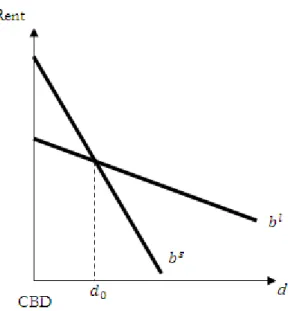
Rent Gradient Law

In order to further understand the idea of hedonic prices, one should take in to account the fact that house attributes are in fact different depending on regional locations. Andersson, Pettersson & Strömquist (2007) highlights a bid-rent model to study the regional differences in household location and decision at a micro-level. The rent-gradient law asserts the likelihood that small houses can be found in the centre, while larger ones can be found further away in the peripheral regions. Figure 2 gives a graphical explanation of the two different curves that represents small and large households. When small households demand little b (size), households will tend to move closer to the Central Business District (CBD) and vice versa. Therefore if d<d0, then the region is dominated by smaller households and after d0, the larger households are dominating.

Figure 2 The Rent Gradient Law

Source: Andersson, Petterson & Strömquist (2007)

Portfolio Price Real Estate

The estimation of asset returns is quite straightforward since one uses the income together with the capital gain and loss. However, the determination of real estate prices is not as easy as it is with for example stocks which are frequently traded in auctions whilst houses are rarely traded. Therefore, estimations can be made annually by using previously purchased properties and use that price as a benchmark for estimating the value of the property still not sold. Also the property can be valued through the method of discounted cash flows which predicts the cash flows of the future and discounting it with respect to the current market conditions (Firstenberg, Ross & Zisler, 1998).

Bubbles and Booms – Estimating Asset Prices

The consequences of series of deregulations and bad timing contributed to the phenomenon of a speculative house price bubble. The bubble is generally created when house prices inflate to such a degree that they cannot be backed by its fundamental value. Therefore, to prevent price bubbles, it is important to be able to determine the true house prices in order to avoid large deviations from the equilibrium value.

Abraham and Hendershott (1996) points out the determinants of real house prices appreciation can be divided into two groups: one that explains changes in the equilibrium and another that accounts for the adjustment dynamics from the equilibrium price. Englund (1998) present evidence on house price determination when house prices are set in an efficient market.

Poterba, Weil & Shiller (1991) finds violations of the standard efficient market theory in which house prices do not behave as efficient asset prices. This is important in order to understand that homeowners can slowly recognize rapid house price appreciations, which repeatedly prevents them from avoiding bubbles. Poterba, Weil & Shiller (1991) therefore states that house prices can be subject to speculative bubbles and are connected to financial markets. This is because falling prices diminishes household worth and contributes to the stress on many financial institutions. Furthermore Hamnett (1989) gives a clear explanation of what occurs within the speculative demand and supply forces in the housing markets. In the short term, house prices tend to rise faster than income. Later, when income rises and surpasses house prices, house prices rise again and increase housing demand rather than what the conventional supply and demand theory suggests. Rapidly rising prices thus generate additional demand, which continues to the point where rising house price cut off the potential demand. At this point, the cycle peaks and reverses as potential buyers realise that they can no longer afford to buy houses. Afterwards the seller’s market then dominates for some years until rising in real incomes and falling house price reach a point where new buyers are attracted into the market again in large numbers. An expression used by Maher (1994) is that price increases caused by inflation promotes a bandwagon effect. This means that those who consider purchasing homes feel pressured to buy before the price rises further and to capitalise on the available gains when selling the home. It should be noted that nominal price changes usually are the basis of their owner-occupiers information when making a decision. Thus examining nominal price change may not be the drawback as it first appears (Maher, 1994).

Portfolio Investments in Housing Markets

For another way to assert different characteristics of regional house prices one should know that size and diversity causes regional growth, which is endogenously stimulated by its local market. This means that a metropolitan region develops faster than the smaller ones. Hence, the investment decisions made in larger agglomerated regions implies a lower risk in housing markets, due to a relatively stable housing demand. This means that when somebody estimates house prices and their investment potential, they need to take into account different expected returns and risks depending on the region. Since high risks imply high potential returns, the expected returns from smaller regions correspond to a higher β-value. The higher β-value presents the relative risk premium, defined as (rM-rF). In Figure 3, the security market line depicts the positive trend of rising risk premiums (Andersson, Pettersson & Strömquist, 2007). Hence, housing companies adjust their portfolios due to the regional differences in size and risk. Spreading the investments enables a diversification strategy that eliminates the regional specific risks. However, this might be possible for larger real estate companies operating in all regional markets, while it may be highly restrictive for local authorities.

Figure 3 Portfolio investments

Source: Andersson, Petterson & Strömquist (2007)

Data and Methodology

The variables selected will be tested through a cross-section analysis in order to highlight which are important and how their importance differs with respect to different time periods and regions. The data that has been used for the regression analysis contains numbers recovered from the extensive supply of statistics by Statistics Sweden (SCB). Here, the author has recovered a series of data from the 290 municipalities within the time range of 1990-2008 to facilitate the possibility of getting accurate results.

However, when retrieving the data, it was broken down into smaller time ranges within 1990-2008, due to changes in the number of municipalities during that period. Today, the municipalities of Nykvarn, Knivsta, Gnesta, Trosa, Bollebygd and Lekeberg have been broken out from their previous municipalities. In order to reach conformity between all data, the six new municipalities where added back to its original municipalities. This reduced the number of observations from 290 to 284 but is not regarded to give any substantial changes in the empirical findings. The data represents eight different variables that will be included in this model in order to measure relevant influences on regional house prices. Since certain data is at the national level these have been amended to account for regional-specific data by using ratios and combinations with other regional data. All monetary data has been adjusted for inflation in 1990’s prices. Since all data are expressed in different units and amounts, all data where recalculated as indices with respect to the first year of 1990. This helps scale down numbers and expresses the real changes rather than the quantitative changes.

Regional House Prices is the dependent variable which will be the main subject of

analysis. The house price movements are not only a controversial subject since its movements depends on many factors but it can be estimated at different levels. When dealing with regional house prices it is important to include as many relevant variables that cause shifts in the house price movements within the Swedish borders. In order to measure

between regions it is important to know that some are less populated than others. The impacts on house prices by Population might therefore be a useful explanatory variable. The Employment variable represents the economic activity of a region that enables some regions to develop with greater importance and have different trends in house prices. The employment data contains the ratio between the regional workers and its population.

Income is also important when taking into account the average income gained by the

regional employees. This, as well as employment is another indication of economic activity and importance between regions and time. Interest costs is the cost of borrowing and is not only of national importance since it can affect the regional population differently. This was calculated by multiplying the house prices with its respective mortgages interest rates and then divided by the average regional income. The House stock variable represents the number of house properties that occupy regional space. This variable is important to explain house prices since it indicates the regional supply of houses provided during different time periods. The number of Sold Houses could vary since it reflects a household’s willingness to purchase a household. This variable therefore helps to understand when the acquisition of houses has been most interesting between regions. The

Internal migration movements by Swedish citizens can occur due to different social,

economical and psychological reasons. This is important in order to understand how households move between regions and affect regional house prices. The External

migration coming from abroad might be an advantage or a disadvantage depending on

where there movements are located. If they are concentrating on large regions, it favours urbanization and if it is dispersed around the country it might be beneficial to all regions. Thus, this makes this variable important to include in the model.

The variables have been given suggested signs with respect to the dynamics model by Wheaton & DiPasquale (1996). The variables are categorized either as demand, which gives it a positive correlation to house prices, or supply which gives it a negative correlation to house prices.

Table 1 Variables and suggested signs

Variables Suggestion Suggested sign

Population When a region’s population increases, the demand for

houses increases as well. + Employment When people are employed,

the affordability to buy a house

increases demand. +

Income As the previous variable, affordability increases demand.

+ Interest Cost When borrowing costs go

down, people can receive more credit and demand to buy more houses thus raising its price.

-House Stock When houses are built, the supply increases which brings

-Sold Houses Sold houses indicate that the housing market is active and

that demand is increasing. + Internal Migration The more concentrated a

population becomes in any

region, the greater the demand + External Migration When regions receive new

inflows of residents, its

demand for housing increases. +

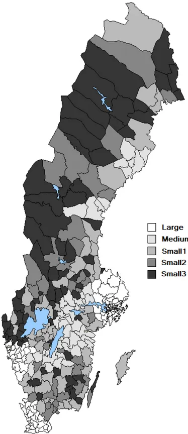
Regional Division

In order to have a well-trusted model, regional division need to be done in a way that each sub-group contains its specific characteristics. The division has been made in five regional groups to specify regional differences in a clear manner. The ranking was made on the basis of employment volume from the mid 1990s. It should be pointed out that the rankings have changed insignificantly during the 1990-2007 period which justifies for this specific period to be chosen. Figure 4 gives a graphical outlay of the regional divisions. The Large region contains the three largest cities Stockholm, Gothenburg and Malmö and all its closest regions that form the three largest FA-regions. It is important to isolate these regions since their economic scale is larger and more dynamic than other regions.

The Medium region was divided by estimating the regions that were ranked after the largest three regions. The second most important regions thus contain Borås, Jönköping, Sundsvall, Umeå, Västerås, Örebro and Östergötland and its closest regions. Here there are less dynamics but still present is some influences of the Large region, whilst being medium-sized may have some effects of its own.

The remaining regions which are regarded as the smaller and minor regions of Sweden were categorized once more into three sub-regions. The sub-regions have the following division in employment:

Small1 (S1) = >10000

The Small1 region is the largest of the small regions. This regions contains a working population larger than 10.000 and as can be seen in Figure 4 below, its vicinity to different regions gives it a mix of influences from larger and smaller markets.

Small2 (S2) = 5000<X<10000

The S2 region is defined as the middle region of the small regions. This region has a working population between 5000-10.000 which gives it greater economic influences than the smallest region but quite small in comparison to the larger regions. Isolating this region defines the town/village categorization that is mandated by local authorities.

Small3 (S3) = <5000

The smallest region S3 contains merely a working population of less than 5000. These workers usually work closely within the village and have more local administrations. The division means small villages that are self-sufficient or quite isolated from the larger markets influences.

Figure 4 Regional divisions in Sweden

Regression Model

The regression is a cross section analysis at a specific time. In this case, this is done four times in order to analyze four specific periods, two recessions and two expansions. The first period reflects the economic crisis in 1991-1994. The second period is the expansionary period 1995-2000 succeeding the crisis. The third period is the crisis of the new decade in 2000-2003. Finally the new expansion followed by the crisis is the period 2003-2007. Since the periods include more than one year, each respective variable contains the difference in data between the last and the first year of the respective period which is indicated by the delta (∆).

Heteroscedasticity

Since the data collected contains series of different municipal data, one need to take into account the different scales and size of the data to avoid any misinterpretations and biasness. Although dividing all 290 municipalities into five subgroups eliminates some biasness, it can be further reassured by testing for heteroscedasticity. Therefore, to further support the empirical results, the regression model needs to fulfil the assumption of homoscedasticity. This means that the variance of each disturbance term is some constant number equal to σ². If this assumption is violated, it means that the regression is heteroskedastic and the regression is inefficient. To remediate this, the regression has been tested for heteroskedasticity test and later corrected its standard errors by using the Robust standard error test indicated by a k on each variable

Correlation Matrix

The matrix allows us to understand if the regression variables are linear dependent. If some variables are perfectly linearly related, then one cannot assess that the variables have different effects on the dependent variable. However, it is almost impossible to find two or more variables that are not correlated to some degree. As long as there are no exact linear relationships between the variables, the validation assumption of the regression is not violated.

∆HP = βkCk + ∆βkPopk + ∆βkEmpk + ∆βkInck+ ∆βkIntCostk +∆βkSoldHk+ (4)

∆βkIntMigk+ ∆βkExtMigrk+ ∆βkHStockk + ε

Hypotheses

At this point, the previous facts and studies bring out some hypotheses. If the regression model is to work at a national level, there should be some consistency in terms of the suggested signs of each variable. If they change, it proves the difficulties of defining certain variables to be descriptive at a national level and stresses its importance to be regionally measured. This will lead us to understand in which sense the variables can be measured regionally. Will it have consistent signs in every region or in every time period? The regression analysis will prove the correctness of the following hypotheses:

Hypothesis 1:

Any variable is consistent at a national level

Hypothesis 2:

Any variable is consistent in terms of region

Hypothesis 3:

Results & Analysis

Here, the empirical findings are analyzed with respect to the theory and previous research. This analysis helps to understand which variables are consistent: nationally, in locations and in time periods. The variables have been corrected for heteroskedasticity which allows for an unbiased and straightforward analysis. Furthermore, to prevent any skewness of the random variables, the robust test has been implemented in the heteroscedasticity approach. The four periods presented contain two sets of recessions and expansions in the 1990-2007 periods. Furthermore, five different regions clarify their individual responses to these four economic cycles. The regions are the Large, Medium, Small1, Small2, and Small3- sized regions which are chronologically ordered and are henceforth called L,M,S1,S2,S3. When testing for correlation, all variables have different correlations in different regions and time periods. However, since the correlation coefficients vary between 30-70%, there is no exact linear correlation which does not reject the results of this analysis. It is understandable that all eight regions are related since they are all region and time-specific and move interdependently within these boundaries.

The R-square indicates the goodness of fit in the models. Some tests gave numbers lower than 0,40 and should therefore not be completely reliable. However, in general, most models are past the 0,40 bracket which fortifies the confidence of the results. Lastly the standard errors have been included to describe the standard deviation of each beta coefficient as an alternative to the p-value for measuring the significance level.

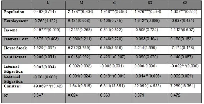
Table 2 First Period – Swedish Crisis Period 1991-1994

*=Significant at 10% **=Significant at 5% ***=Significant at 1%

The first period represents the first crisis period described in the background section and contains 79 observations. Starting with the Population variable, it can be noticed that its beta values are relatively high. As suggested, the signs are quite correct except for one beta

value in the L region. But one should keep in mind that the periods reflect different economic situations, thus one can not expect the variables to be uniform in all regions. However, as Mankiw & Weil (1989) and Maher (1994) suggests, governments can play a role in restricting housing. This must have been relevant in this case particularly for the larger markets since they were in need of preventing the crisis to exacerbate. It can further be noticed that most betas are significant which generally certifies the Population variable’s strength in the model. The Employment variable appears to have relatively high beta values as well indicating its importance in the model. Furthermore, their signs are as suggested indicating that all regions purchased houses when more of its population was in the workforce which was the reason why the crisis worsened (Finocchiaro, 2007). The Income variable is rather small in its beta values in this period. Here, the suggested signs are quite different. In the first period, it appears that the income betas in the M, S1 and S3 regions have an opposite effect on the house prices. This states that more income is not crucial for house prices to rise. Despite the workings of the four-quadrant diagram presented by Wheaton & DiPasqual (1996), they also bring forward the importance of the market participants’ expectations. Thus, during this crisis period, the optimistic expectations that positively relate house prices to income were not present in these regionsThe Interest Cost betas is as well as the Income variable quite low in the first period. Here the suggested correlation between the Interest Cost variable and House Prices is negative. In the first period, the L and the S3 region are the only ones that satisfy this assumption. Evidently for regions M, S1 and S2, higher credit prices will not prevent house prices from rising. The reason why these regions have reverse signs is mentioned by the Ripple Effect (Macdonald & Taylor, 1993). The geographical distance to the most economically active regions determines the impact and time that it is caused on another region. While people in the L region have become discouraged from higher credit costs during these crisis years, it has not yet inflicted the smaller regions in the same way. The S3 region however, is more sensitive than other regions to sudden changes in interest rates whereby the reaction is as expected. The House Stock betas are rather different between regions and the suggested signs are not all fulfilled. In this crisis period, the House Stock increase is not lowering house prices in the L region. Here, the conventional economic theory that more supply lowers prices is violated. But Carol & Barrow (1994) states that larger regions do act independently from other regions. The surge in prices was already underway in the most economically important regions and could not be slowed down easily despite larger housing stock. The other regions seem to act as the supply and demand theory suggests whereas the lower sized region are greater in scale. The Sold Houses variables have less scale size than many variables. In this period, the S3 region is negatively correlated to house prices. As the conventional demand theory suggests, sold houses should indicate the demand of houses and thus raise its prices. However, for S3 when houses are being sold, the prices do not rise. As mentioned earlier, the smaller regions weak responses to the economic crisis caused by the larger regions, asserts further that the smaller market did not suffer from house price rises at this time. One should remember that houses differ, especially between regions. Wheaton & DiPasquale (1996) states that hedonic price explains the difference in house price due to its attributes. As could be expected, the larger regions have very different attributes from the smaller regions so the house prices and its demand should not always apply for the whole country. Firstenberg, Ross & Zisler (1998) says that the continuous estimation of house prices can be quite sluggish and are therefore discounted with respect to a benchmark from other sold houses. However, the estimation of house prices can be quite difficult since the smaller houses sold can lack similarities in quality for the same demanded houses in the other regions. Furthermore, Andersson, Pettersson & Strömquist (2007) recognizes differences in house sizes and distance which is

another indication of house prices differences. The Internal Migration variable has a very small influence on house prices. Within the country, the migration in the S2 and S3 regions seems to have affected the house prices negatively in the first period. As Cameron (2005) suggests, the migration helps understand relations between housing and labour markets. Thus, due to the urbanization that occurs, the labour market is smaller and the internal migration in smaller regions is so insignificant that they hardly affect the house prices. Likewise, the external migration betas do not show much impact. Another similarity is that the house prices are affected by how these immigrants contribute to the labour markets since this stimulates the economy (Cameron, 2005). The migration helps understand relations between housing and labour markets Furthermore, the minus signs in the L and S2 reflects the current crisis inability to provide jobs to the inflow of immigrants.

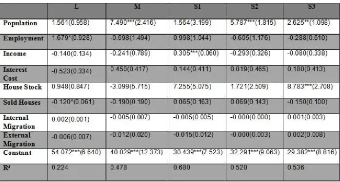
Table 3 Second Period – Expansion Period 1995-2000

*=Significant at 10% **=Significant at 5% ***=Significant at 1%

Here the regression contains 46 observations. The Population variable seems again to have quite strong beta values. In this period they all work as suggested in all regions and are therefore consistent in its movements. More residents are again causing house prices to rise, however in this case the rise contributes to the expansion of the economy. The Employment variable is quite strong and had a reverse effect on the L market. As previously noted in the Population variable, the government intervention has had a long-term repercussion on this new population when they years later started new jobs. The S3 market also had a reverse effect on their house price market. However, Wheaton & DiPasquale (1996) brings up the fact that regions have no borders and if one place is more attractive, people search for greater prosperity in those regions. Leaving the less attractive regions behind, causes their house price market to contract despite its new but smaller employment numbers. Different regions vary greatly in their economies in different times. When it comes to the Income variable, its values are rather strong which certifies its value in this period. As opposed to the case of the first period, all small regions except for the S2

region changed their expectations to an optimistic future. The interest cost variable has a relatively weak beta scale to the former variables. One can again refer to the Ripple Effect regarding the Interest Cost variable to understand that the changes from the both extremes of the L and the S3 regions in the first period have now affected the M and S2 regions. When the effects have been transferred to the other period, the scale has gone up even more, which characterizes the Ripple Effect with a rolling snowball effect. The expansion period that followed the 91-94 crisis have led to even greater house prices whilst the S3 region is the only one in period two that has remained sensitive to house constructions prices. The House Stock variable has relatively large beta values which gives it great power in this model. In comparison to the first period, other regions have now experienced drawbacks of overproduction were the supply of housing production does not bring down the price. The Sold Houses variable has a low value in relation to the other variables. The signs are as suggested except for the S2 region and act counterproductive to the other regions after the crisis. The Internal Migration is recognized as having one of the lowest values betas in all regions. It is marked with the same pattern as the one in the first period except for the S2 region which is neutral in this case. The External Migration is low as well as the Internal Migration and here the signs are as in the first period for the L an S2 market including for the M region as well.

Table 4 Third Period – IT-crisis period 2000-2003

*=Significant at 10% **=Significant at 5% ***=Significant at 1%

The third period which included 49 observations, represents the IT-crisis. The Population variable is like in the second period consistent in all regions. The Employment betas are rather high here as they have been previously. Its effect is reversed in the S1 and the S2 market. This is possibly because the new economic crisis ruined many small investors where many jobs were created in enterprises that lacked a real fundamental value. The Income betas are relatively high and here a negative expectation is present as it was in the second period. The Interest Cost betas values are moderately high. The credit costs have gone down in all except for the S1 region that was never affected before. As previously

noted, the stock market influenced a lot of small investors which at this time have been relatively sensitive to the interest rates and its credit loans. Due to its higher scale than other regions, the previous wave from the Ripple Effect might have had its impact here as well. The House Stock here is rather high meaning a powerful influence in the model. The crisis period between 00-03 has discouraged house prices to fall due to higher housing supply. In fact, the positive correlation between housing supply and house prices in the S1 and S2 regions seems to have been exacerbated even further. Even after the actual house crisis in the 1990s, the future prices overshoot the construction which is defined as the exogenous expectations explained by Wheaton & DiPasqual (1996). As what happened with the S2 region in the second period, the Sold Houses variable has negative sign in the M and S1 regions during this period and low beta values. The Internal Migration variable has as in the other cases a very low beta values. The M region and the S3 region were badly affected in employment by the IT-crisis and caused a greater inflow of people to be counterproductive on house prices. Finally, regarding the External Migration variable, the L region and the S2 regions seem to have recuperated from its previous labour market. However, the M, S2 and S3 region with small size investors faces problems to cope with its job opportunities for its external migration.

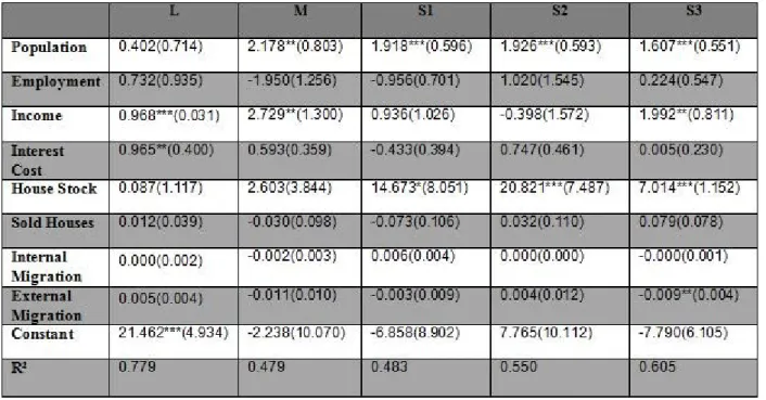
Table 5 Fourth Period – Expansion Period 2003-2007

*=Significant at 10% **=Significant at 5% ***=Significant at 1%

Finally, the fourth period presents the aftermath of the last economic crisis. Here the Population variable has again high beta values and regional consistency in house price reactions. The Employment variable showed that the M, S2 and S3 regions had reversed effects on house prices. The Ripple Effect stated by Macdonald & Taylor (1993) could explain the sluggishness of the peripheral regions to react on house prices. The previous crisis of the middle sized region affected the smaller regions years later. In addition, the M region was still inadequately recovered as well. The Income variable, betas are rather weak and S2 have kept its negative position. The negative sign was not only due to the expectations, but by the IT-crisis period that affected all but the S1 period. The Interest

Cost variable had fairly strong beta values this period. The L region is the only one that follows the suggested sign pattern. Here, the region has been affected by two crises which have left greater awareness among its inhabitants to be more careful with interest rates effect on house prices. House Stock is important in this case due to its higher beta values. The M region is the only region that is now acting as conventional theory suggests. The small investors of the middle sized region have now been discouraged by over constructing after undergoing hardships of negative investments. Concerning the Sold House variable the fourth region shows that the L, M and S3 region have underwent negative reactions as suggested. The reasons are the awareness of the larger region to be more austere and the smallest region has increased sensitivity than before. The betas are quite low as before. The Internal Migration in the fourth period is dominated by negative effects in the M, S1 and S2 period and again low betas. Here the after-effects of the previous crisis period have left a pattern of low stimulations in house prices due to internal migration. Lastly the External Migration shows an aftermath of the last crisis with all regions but the S3 region to have problems providing jobs for its immigrants.

To finish with the last variable in all periods, the constant represents all other variables left behind. As can be seen, the values of the betas are quite high so it leads us to realize that some other variables are influential in order to understand more about the complex mechanics of the regional house price analysis. The fact that regional house price investigations can be time and region-specific proves that its workings are interconnected with similar and different factors. These factors are not only extensive to retrieve but also subject to changes which require continuously rigid examination.

From this analysis, the results can be stated in accordance with the hypotheses. First, since there is no absolute consistency for any variable at a regional and time specific perspective, no variable can be measured at a national level. Thus Hypothesis 1 is rejected which has brought evidence to the fact that the national house price data are just simplified but inadequate information. This conception is of much concern for portfolio investors when pondering about different returns in real estate investments (Andersson, Pettersson & Strömquist, 2007). Second, most variables have some occasional changes in their signs due to the constant dynamics of the economic cycles and its regional responses. However the Population variable is proven to be quite consistent in its signs for almost all time periods. In every case except for the L region in the 91-94 period the other regions have the same signs throughout all periods investigated. The Employment variable proves to be consistent in all 5 regions for the 91-94 period. Thus, we can find evidence of some regional and some time consistency. We can therefore not reject Hypothesis 2 and Hypothesis 3. From this we can understand that national measures of variables are not useful when going to the bottom of house price formations. Furthermore, the Population and Employment variables are useful for measuring the formation of house prices at a regional level. In fact, other variables with similar characteristics can contribute even more to extending the field of regional house price formation.

Conclusions

Previous research states that if enough data exists, the housing market can be better explained if it is regional specific rather than national. This study has investigated regional house prices which may bring out the importance of the approach for estimating house markets. By observing the dynamics of house price markets and learning the fundamentals about the Swedish economy, this thesis divides the Swedish regions into five regional groups and performs twenty different cross-section analyses. Furthermore, as much as location differences are important, the specific time periods are also essential to predict or determine house price movements. The cyclical movements have shown similarities and differences between explanatory variables by discerning variable characteristics in time and regions. The Betas values indicate the sensitivity for each variable and thus to what extent it changes. For the Population and Employment, variables are among the highest. This is later followed by the Income, Interest Cost and House Stock whose beta values changes over the periods. Lastly, the Sold Houses, Internal Migration and External Migration are variables with quite a low beta. Furthermore, throughout the analysis, certain characteristics are discerned. The Population and Employment variables are affected by the government policies. Furthermore, Employment and Interest Costs show tendencies of the Ripple Effect. The Income and the House Stock variable are influenced by expectations and both migration variables are connected with the labour markets. This shows the diversity of the different factors that may affect different variables in regions and time. One should also take into account the sensitiveness of the smaller regions and the middle sized regions greater exposure to the IT-crisis. In conclusion, Hypothesis 1 is rejected, meaning there is no consistency in signs for the whole time span and for all regions. The Hypothesis 2 and 3 is however not rejected since the Population shows consistency in regions and Employment show consistent signs in time. When dealing with the significance values it can be concluded that the Population variable is most significant whilst the other significant variables are ranked in the chronological order: Income, House Stock, Sold Houses, Employment, Interest Cost, Internal Migration and External Migration. As previously mentioned, the vastness of regional house prices studies extends the scope of investigation to a whole spectrum of different influences. This thesis has led to the conclusion that investment decisions should be taken at a regional level. Furthermore, Employment and Population are important variables for measuring house prices at a regional level. Despite weak indications of other variables, there are still other variables that can explain how house prices are formed in a regional perspective. With this intriguing observation, this investigation can open a new field that relates to house prices relation to regions and time.

Suggestions for Further Research

When performing tests on house price dynamics it is understandable that some variables may be omitted or left out. When testing for other variables, one can possibly find other important factors that help explain more about house prices in time and location. Therefore, further research should be made in order to complement this study and give a greater insight into this problem.

The study has had its limitations when dividing Sweden into five regions and choosing four cyclical periods. Although this brings out twenty regressions, more investigations can be made by dividing groups and time periods into more than five and four respectively.

References

Abraham, J. M., & Hendershott P. H. (1996). Bubbles in Metropolitan Housing Markets.

Journal of Housing Research, Volume 7, Issue 2, 191-207.

Cameron, G., Muellbauer, J., & Murphy, A. (2005). Migration within England & Wales and The Housing Market. Economic Outlook, Vol. 29 Issue 3, 9-19.

Cameron, G., Muellbauer, J., & Murphy, A. (2006). Was There A British House Price Bubble? Evidence from a Regional Panel. CEPR Discussion Papers, No 5619.

Carol, A., & Barrow, M. (1994). Seasonality and Cointegration of Regional House Prices in the UK. Urban Studies Vol. 31, Issue 10, 1667-1689.

Case, K. E. & Shiller, R. J. (1990). Forecasting Prices and Excess Returns in The Housing Market. Areuea journal, Volume 18, no 3, 263-273.

Drake, L. (1995). Testing for Convergence between UK Regional House Prices. Regional

Studies, Volume 29, Issue 4, 357-366.

Englund, P., & Ioannides, Y. M. (1997). House Price Dynamics: An International Empirical Perspective. Journal of Housing Economics, Volume 6, Issue 2, 119-136.

Englund, P.(1998). Improved Price Indexes for Real Estate: Measuring the Course of Swedish Housing Prices. Journal of Urban Economics, Volume 44, Issue 2, 171-196.

Finocchiaro, D. (Ed.). (2007). Essays on macroeconomics. Institute for International Economic

Studies. Monograph Series No. 61.

Giussani, Bruno., & Hadjimatheou, G. (1991) Modelling regional house prices in the United Kingdom. Papers in Regional Science. Volume 70, Number 2, 201-219.

Goodman, A. C. (1976). Hedonic Prices, Price Indices and Housing Markets. Journal of urban economics. Volume 5, Issue 4, 471-484

Hamnett, C. (1989) Regional Variations in House Prices and House Price Inflation in Britain. Journal of Property Valuation and Investment, Volume 7, Issue 4, 342-360.

Jud, G. D., & Winkler, D. T. (2002). The Dynamics of Metropolitan Housing Prices. The

Journal of Real Estate Research, Volume 23, Issue ½, 29-46.

Macdonald, R., & Taylor, M. P. (1993). Regional House Prices in Britain: long-run relationships and short-run dynamics. Scottish Journal of Political Economy, vol. 40, Issue 1, 43-55.

Maher, C.(1994). Housing prices and geographical scale: Australian cities in the 1980s.

Urban Studies, Vol. 31 Issue 1, 5-27.

Mankiw, N. G., & Weil, D. N. (1989) The Baby Boom, The Baby Bust, and The Housing market. Regional Science and Urban Economics, Volume 19, No. 2, 235-258.

Poterba, J. M., Weil, D.N., & Shiller, R. (1991). House Price Dynamics: The Role of Tax Policy and Demography. Brookings Papers on Economic Activity, Vol. 1991, No. 2, 143-203.