Closed-End Funds and their ………
Net Asset Value over time
(Understanding the (relationship) of Net Asset Value (Discount/Premium) to Closed-end funds’ stock prices)
BACHELOR THESIS WITHIN: Economics & Finance NUMBER OF CREDITS: 15 ECTS
PROGRAMME OF STUDY: International Economics
A study of the relationship between Swedish
closed-end funds’ market prices and their
underlying assets over a period of time.
Bachelor Thesis in Economics & Finance
Title: Closed-End Funds and their Net Asset Value over time
Authors: Erik Cederberg and Linus Schnitzer
Tutor: Michael Olsson
Date: 2020-05-18
Key terms: Closed-end fund, Net Asset Value, Mean Reversion, Closed-end fund discount,
Stock market, Investment strategy, Cointegration, Error Correction
Abstract
Closed-end funds (CEFs) are popular investments amongst the Swedish population as they provide diversification to investors and have in many cases historically outperformed the market. In decid-ing whether to invest in a CEF, the method of valuation differs from classical financial ratios used to value most companies, as the revenue-bringing operations differ significantly. The Net Asset Value (NAV) per share is compared to the market price per share of a CEF, to determine if the share is traded at a discount or premium.
The purpose is based upon the rationalization that a share’s market price and the value of the closed-end fund’s underlying assets cannot drift too far apart from each other. In other words, the discount cannot drift too far from its mean over time, as there would be an upward pressure on the share price if the NAV-discount is large, and a downward pressure on the share price if the premium is large.
Tests of unit roots and cointegration are applied and analysed in the light of previous findings for discounts in CEFs.
Our findings show that the majority of selected CEFs’ prices and NAVs have long-run equilibrium relationships. Additionally, the discount appears to be stationary over time for the majority of CEFs, supporting the notion of mean reversion in the discount. For certain Swedish CEFs, the findings allow for investment decisions to be made upon the deviation from the mean.
This study contributes to previous research done on the topic of mean reversion in the financial market as it finds statistical evidence of mean-reverting process for the NAV-discount of Swedish CEFs. The thesis also provides additional value to the plethora of research provided in the financial field as it specifies its findings to the Swedish market of CEFs.
Table of Contents
1.
Introduction ... 1
2.
Theory ... 5
2.1 Literature Review ... 5
2.1.1 Net Asset Value-Discount ... 5
2.1.2 Mean Reversion ... 6
2.1.3 Unit Root ... 7
2.1.4 Integration and Cointegration ... 8
2.1.5 Error correction mechanism ... 9
2.1.6 Behavioural Finance ... 10
2.2 Hypotheses ... 10
3.
Variables and Data ... 11
3.1 Variables ... 11
3.2 Data ... 11
4.
Method ... 16
4.1 Testing process for Hypothesis 1 ... 16
4.1.1 Fisher-type tests ... 16
4.1.2 ADF tests and PP tests ... 17
4.1.3 Engle-Granger (EG) tests and ECM ... 17
4.1.4 Johansen tests and VECM ... 19
4.2 Testing Process for Hypothesis 2 ... 20
5.
Results and Analysis ... 21
5.1 Hypothesis 1 Statistical Findings ... 21
5.1.1 Fisher-type tests ... 21
5.1.2 ADF tests and PP tests ... 21
5.1.3 Engle-Granger (EG) tests and ECM ... 23
5.1.4 Johansen tests and VECM ... 24
5.2 Hypothesis 2 Statistical Findings ... 25
5.2.1 Fisher-type tests ... 25
5.2.2 ADF tests and PP tests ... 25
5.3 Analysis ... 26
6.
Discussion and Conclusion ... 30
Reference List ... 33
1. Introduction
This chapter provides the reader with relevant information on the topic of Closed-End Funds (CEFs) and presents the reader to the purpose of the research. Additionally, back-ground regarding relevant statistical tools and measurements are specified and discussed.
Closed-end funds (CEFs) have a noble heritage within the financial world. According to Anderson, Born and Schnusenberg (2010), a CEF is one of many investment vehicles avail-able on the financial market and the origin of the very first is divided amongst historians, but one of the earliest to be introduced to the U.S. market was the Boston Personal Property Trust in 1893. Even though the popularity of closed-end investment companies has varied greatly since then, the number of investment companies in the form of funds and trusts has grown remarkably as the wealth of the public has increased. A CEF is an investment com-pany that manages and provides a portfolio consisting of financial investments, for instance, securitized assets, real estate, or other financial instruments. A benefit of the presence of CEFs is that investors can indirectly access more illiquid securities, such as unlisted shares, which in the absence of CEFs would be difficult. A closed-end fund differs from an open-end fund in the sense that it has a fixed number of shares outstanding through the initial public offering that are traded on an exchange. Hence, the share price is determined in the secondary market, allowing for differences between the share price and the value of the un-derlying assets (SEC, 2013). The open-end fund, however, continuously offers shares to the market that is set by the NAV of the fund at that particular point in time.
The Net Asset Value is the total amount of assets of an entity minus its liabilities, i.e. the liquidation value of the outstanding shares (Anderson et al., 2010). It is a simple valuation of the net worth of the company. The total NAV can then be divided by the number of shares outstanding to get a per-share basis. By comparing the NAV per share relative to the market price of a share in the company, it is determined whether the share is traded at a discount, premium, or at fair value. If the price of the share is below the NAV, the share is traded at a
discount. Conversely, if the share is traded above its NAV, it is said to trade at a premium. The
discrepancy is calculated in percentage as (𝑁𝐴𝑉 − 𝑃𝑟𝑖𝑐𝑒)/𝑁𝐴𝑉, and is called the NAV-discount. As the revenue for mutual funds, exchange-traded funds and, real estate investment trusts (REITs), as well as CEFs, does not come from selling goods and services, but rather from holding assets whose value and cash flows generate profit for investors, the
NAV-discount is a more commonly used financial ratio rather than the more classical P/E ratio for evaluating a company.
Historically, CEFs have been traded at discounts for most of their existence. This has been empirically examined in previous research and is established as the “closed-end fund puzzle”. The name stems from the conflict of CEFs’ NAV-discounts to concepts in neoclassical fi-nance (Cui, Gebka & Kallinterakis, 2019). Because of the main revenue-bringing operation for a CEF is to invest in other companies, the CEF’s fundamental value is expected to equal the value of its assets. Since CEFs mostly trade at discount, investors continually buy the underlying assets for a price lower than if they would buy the portfolio’s securities individu-ally (ignoring transaction costs). Thus, a closed-end fund’s market value is not equal to the value of its assets, which allows for arbitrage opportunities, where an investor can take a long position in a CEF trading at a discount, and take a short position in the underlying portfolio. However, such a strategy is problematic to implement. Lee, Shleifer and Thaler (1991) iden-tify practical problems with this arbitrage strategy. If the CEF makes changes in its portfolio, the arbitrageur must follow by making similar changes to his/her own portfolio consisting of short positions, to correctly mirror the position. This comes with difficulties regarding timing in the transactions. Additionally, hedging comes with costs, hence not all gains are profits.
By the end of 2019, approximately 1.9 million Swedish private investors owned shares in Swedish corporations listed on any Swedish exchange or trading platform. That is approxi-mately 18 percent of its entire population. Swedish individuals represent the largest group in terms of number of unique owners, 86 percent, but they only account for 12 percent of the total market value (Euroclear, 2020). Albeit not preventing systematic risk, diversification can reduce unsystematic risks specific to each individual stock (Markowitz, 1952). While the average number of different stocks per individual in Sweden is 4.1, the share of private in-vestors owning stock only in a single company is 44 percent (Euroclear, 2020). A reason for closed-end funds being a popular choice amongst individual investors may be that it provides diversification for investors.
Owner statistics from Avanza Bank (2020-02-04) show that the most owned share among the bank’s customers is Investor B with 94,792 owners. The fourth most owned stock is
Kinnevik B, with 61,474 owners, both of which are Swedish CEFs. Additionally, data col-lected from Nordnet AB (2020-02-05) displays that out of their 913,600 (2019) active cus-tomers, there are 90,602 customers who own shares in the 13 most common Swedish CEFs. Alexander Gustafsson (February 5, 2020), investment coach at Nordnet Bank, shows figures that coincide with those of Avanza as out of the Swedish listed CEFs, Investor B is the most owned stock out of the Swedish CEFs with 19,123 owners and Kinnevik B as the second most owned stock with 13,400 owners. This data to some extent coincides with findings by Weiss (1989), that closed-end funds are mostly sold to individual investors, not to institu-tions. Also, Lee et al. (1991) found that in 1988, institutional ownership in their sample of twenty U.S CEFs was only 6.6 percent, in comparison to 26.5 percent for the smallest 10 percent of stocks on the NYSE, and 52.1 percent for the largest 10 percent of NYSE stocks. Additionally, they found that the majority of trades in CEFs were less than $US 10,000 (equivalent to slightly above $US 22,000 in 2020, adjusted for inflation). A potential reason for the popularity of CEFs amongst the general public may not only be contributed to the advantage of diversification, but also the remarkable growth that they have achieved. With data obtained from Börsdata, from the 31st of January 2000 until the end of 2019, the five
largest Swedish CEFs ranked by market capitalization have seen a price increase per share of 669 percent on average. A blunt, non-risk-adjusted comparison to the OMXS30 shows a development of 54 percent for the same period and for the index SIXRX where dividends are included, an increase of 317 percent. These returns might carry an explaining factor for the high interest of CEFs amongst the Swedish savers.
Earlier studies by Malkiel (1995), Thompson (1978) and Pontiff (1997) indicate an arbitrage opportunity of investing in a CEF when the discount is historically large and exiting the investment when the discount has narrowed. These actions result in excess returns for the investor. However, the fundamental idea behind this strategy is based upon the theory of mean reversion in the discount. If no such evidence of a mean-reverting discount is to be found, the strategy can be dismissed. These previous studies are based on U.S. data, which makes a comparable study for the Swedish market justified, as many individuals invest in Swedish CEFs. As the purpose of the paper is to find if there is evidence to support the theory of accordance between the CEF’s trading market price and its historical NAV-discount, it is relevant to highlight the dispute between active versus passive investing that has gained a lot of attention recently. As the management of a CEF does not try to replicate an index, it would be considered as an active investor. The conundrum of which strategy is
superior has bothered investors for a long period of time, during which several studies regarding the subject have been conducted. Swedroe (2011) states that over time, actively managed funds have a hard time matching the returns of an index fund after taxes and fees. This raises the question of how is it that a market for funds other than index replicates exists? Should they not have been ousted by the much cheaper financial instrument such as an exchange-traded fund to mirror the market and perform, if not better, at least the same as an actively managed fund with high commissions, seemingly paying for a service not required? Important to bear in mind is that the time period of the investment complicates the comparison against an index-mirroring investment as an active investment seldom consists of only a single purchase and single sale. An explaining factor for why there is an opportunity of profit higher than the index for an investment in an actively managed fund could be that there are price imperfections. This is where the purpose of this research stems from. Considering the possibility of price imperfections in the financial market, a conclusion of mean reversion for a CEF’s discount can then lay the foundation of a viable investment strategy for an investor to exploit the temporary deviation from the long-term historical mean.
With regard to the absence of research of mean-reverting tendencies in discount-to-NAV for Swedish listed CEFs, the purpose is to investigate that relation. Put differently, the aim is to examine if there is a statistical pattern of the NAV-discount or premia and if it shows signs of mean-reverting behaviour. After conducting several statistical tests of relevant variables this paper finds evidence that suggests cointegration between a CEF’s price and its net asset value. Additionally, a conclusion can be made that the NAV-discount appears to be stationary over time, evidence supporting the hypothesis of mean reversion in the discount for Swedish CEFs.
The subsequent chapters are organized as follows: Chapter 2 presents the theoretical framework which explores relevant theories and their previous applications in research connected to NAV-discounts and within areas of close proximity. Chapter 3 describes the data and variables for this study. Chapter 4 is reserved for the methodology of the study and the testing process. In Chapter 5, the empirical results are presented and analysed. Thereafter, Chapter 6 is devoted to a discussion of the findings followed by suggestions for future studies.
2. Theory
In this chapter, previous studies on the topic are recognized and evaluated. Theories such as mean-reversion and unit root processes are presented and critically interpreted. Furthermore, relevant statistical tools and measurements are discussed and described in order to establish the framework of the research. Ultimately, the hypotheses of the research are declared.
2.1 Literature Review
Here, previous research with relevance for this study’s theoretical framework and statistical methods are presented. Firstly, the NAV-discount and its determinants are explored. Sec-ondly, background regarding commonly used procedures is presented and described. Lastly, the role of behavioural finance is discussed.
2.1.1 Net Asset Value-Discount
There is a considerable amount of research on the topic of Net Asset Value for different financial instruments with the main focus on international open and closed-end funds (see Bhargava, Bose and Dubofsky (1998), Chalmers, Edelen and Kadlec (2001)), real estate com-panies (see Danckwardt-Lillieström and Storm (2015)) and a variety of Real Estate Invest-ment Trusts (REITs) (see Rehkugler, Schindler and Zajonz (2012) and Patel, Pereira and Zavodov (2009)). As the Swedish listed closed-end funds have been left out of the discussion regarding mean-reverting tendencies, there is a void to be filled regarding the NAV discrep-ancy amongst those CEFs.
Malkiel (1995) argues that the reason for the divergence between the NAV and the share price can depend on several factors such as tax deductions, payout policy, owner structure, and turnover. The reason for shares to be traded to premium relative its NAV can be due to a large share of its underlying assets being non-securitized thus providing the investor with the possibility to get access to the non-listed asset through the listed company or fund. Ac-cording to Clayton and MacKinnon (2001), size, debt to equity ratio, and liquidity are ex-planatory variables for a premium to NAV for REITs. In a master’s thesis, Egerot and Hag-man (2011) found that the dividend payout ratio has a positive effect on the NAV discount for Swedish CEFs, which could possibly be explained by the absence of profitable invest-ment opportunities. That would indicate a low potential for the CEF since its purpose is to provide shareholders with profits by investing in other companies. This result coincides with
Gasbarro, Johnson and Zumwalt (2003), who mention that CEFs with poor management performance or unsuitable investment strategies can exhibit large discounts continually, and thus cannot be expected to mean-revert. Gasbarro et al. (2003) examine if price and NAV for U.S. closed-end funds are in any way correlated and if so in what direction. They conclude that most of the CEFs included show tendencies of mean reversion caused by both the NAV and the price.
2.1.2 Mean Reversion
Mean reversion in statistical terms can be referred to as a stationary process. Gujarati and Porter (2009) define the stochastic process to be stationary based on three conditions; if the mean and variance are constant over time and that the covariance of two different time pe-riods is only dependent on the distance between the time pepe-riods and not the time at which the covariance is computed. If the three parameters are constant, it is defined as time-invar-iant, i.e. it tends to return to its mean. As the variance is finite for the stochastic process, the mean will therefore not drift too far away from its historic mean. If the condition of constant variance does not hold for the stochastic process, it is referred to as a nonstationary time series.
The fundamental theory is that there is an arbitrary opportunity as the NAV-discount of a CEF diverges from its historical average and ought to revert. The theory is based upon the phenomenon of mean reversion. There are numerous studies revolving the topic for the occur-rence of mean reversion in the stock market. Exley, Smith and Wright (2002) investigated if there is any trace of mean reversion in national equity markets based on the dividend yield. The initial evidence suggests that for the five chosen equity markets, a one percent higher than average yield results in a six percent higher expected return for the upcoming year, seemingly supporting the hypothesis of mean reversion. To investigate whether the mean of a stock price is of relevance, Poterba and Summers (1988) argue that depending on a few characteristics, there is no statistical evidence that share prices in a time series are independ-ent of each other. According to Fama and French (1988), there are ambiguous results of mean reversion in stock prices depending on the time frame applied. They conclude that for a longer period of time, evidence suggests that the variation of returns is dominated by ran-dom-walk price components, coinciding with the hypothesis that the price of stocks has a slowly decaying stationary component. However, they also state that in a shorter time period,
there is a lack of evidence of negative autocorrelation. The effect is more evident for port-folios consisting of smaller firms in comparison to larger firms where a smaller fraction of the return variation can be accounted for by price prediction based on mean reversion. Po-terba and Summers (1988) and Fama and French (1988) provide evidence for mean reversion in prices of US stocks. Similarly, Patel et al. (2009) investigate the mean-reverting phenome-non in REITs’ discount to net asset value in the UK between January 1990 to February 2009, and the results show mean-reversion. Contrarily, Gasbarro et al. (2003) found that not all funds they investigated had mean-reverting discounts, and conclude that mean-reverting dis-counts are fund specific. This means that excess returns cannot be generalized to every fund, but that there are characteristics individual to each fund that allow for such returns.
2.1.3 Unit Root
For determining if a variable is mean reverting, some statistical terminology and methods need to be discussed. A unit root stochastic process refers to a time series that is nonstation-ary. In a unit root stochastic process, any shock in the dependent variable is permanent, and will thus tend not to return to a trend over time. Consequently, past observations are of no use to conduct reliable forecasting (Gujarati & Porter, 2009). For this study, if a CEF’s NAV-discount does not possess a unit root, it will be considered to be mean-reverting over time. Consider the AR(1) model:
𝑌𝑡= 𝜌𝑌𝑡−1+ 𝑒𝑡 , 𝑡 = 1, 2, …, (1)
where 𝑌0 = 0, |𝜌| ≤ 1 and {𝑒𝑡} is a series of independently and identically normally
distrib-uted random variables with a mean of zero and constant variance 𝜎2, that is 𝑒
𝑡𝑖𝑖𝑑~(0, 𝜎2)
(Dickey & Fuller, 1979). To see why a unit root process in nonstationary, consider the fol-lowing properties of the model in Equation 1, based on 𝑌𝑡 = 𝑌0+ ∑ 𝑒𝑡, that is 𝜌 = 1:
𝐸(𝑌𝑡) = 𝐸 (𝑌0+ ∑ 𝑒𝑡) = 𝑌0 (2)
𝑉𝑎𝑟(𝑌𝑡) = 𝑡𝜎2. (3)
Evident from Equation 2 is that the mean is time-invariant. On the contrary, as Equation 3 shows, the variance increases over time. If |𝜌| < 1, the time series 𝑌𝑡 would be stationary as
𝑡 → ∞. However, if 𝜌 = 1, the time series is called a random walk, also known as a unit root, and is no longer stationary. A noteworthy assumption for the Dickey-Fuller (1979) test to be applicable is that the error terms, 𝑒𝑡, are identically and independently distributed. If not,
there is a substantial risk of serial correlation in the error terms. To cope with this problem, Phillips and Perron (1988) constructed a test with non-parametric statistical methods without the requirement of adding lagged difference terms. The advantage of the Phillips-Perron test is that it gives local asymptotic power functions and also shows more robustness to unspec-ified autocorrelation as well as heteroscedasticity in the disturbance process. Note that testing the stationarity of panel data, regardless if it is conducted with an ADF or PP-test, it requires a certain modification to the original test. This is known as a Fisher-type unit root test which will be explained in further detail in Chapter 4.
2.1.4 Integration and Cointegration
Time series have the ability to be integrated, meaning that they tend to move towards a common long-term equilibrium while still allowing for short-term dispersion. However, some time series may have to be differenced to cope with the problem of drift. If a time series 𝑌𝑡 has to be differenced 𝑑 times in order to be stationary, it is said to be integrated of
order 𝑑, denoted as 𝑌𝑡~𝐼(𝑑). Most economic time series are only stationary after taking their
first differences, i.e. they are 𝐼(1) (Engle & Granger, 1987). If a time series is stationary in its original form, it is said to be 𝐼(0) (Gujarati & Porter, 2009). If the components determin-ing a CEF’s NAV-discount are 𝐼(1), and the discount itself is mean-revertdetermin-ing, it should fol-low that the components share a common stochastic trend. Further, if two time series 𝑌𝑡 and
𝑋𝑡 are both integrated of the same order, it generally follows that the linear combination
𝑍𝑡 = 𝑋𝑡− 𝑎𝑌𝑡 will be integrated of that same order. They can, therefore, be referred to as cointegrated time series (Engle & Granger, 1987). Combining time series that are integrated of different orders has its conditional properties that vary depending on the combination in question. In this study, the focus lies exclusively on combinations where both price and NAV are integrated of the same order. To statistically determine if the components of the NAV-discount do share a common stochastic trend, tests of cointegration are conducted. An al-ternative test to examine the question of cointegration between two time series was proposed by Søren Johansen (1988). The Johansen model does not only examine if two variables are cointegrated but also the characteristics of the cointegration. The model is based on the
presence of cointegration vectors 𝑟. Consider a sequence {𝜀𝑡} of independently and
identi-cally normally distributed p-dimensional Gaussian random variables with mean zero, then the process of 𝑋𝑡 can be defined accordingly:
𝑋𝑡= 𝛱1𝑋𝑡−1+ ⋯ + 𝛱𝑘𝑋𝑡−𝑘+ 𝜀𝑡. (4)
𝑡 = 1,2, … , (5)
for given values of 𝑋1−𝑘, … , 𝑋0 where k represents the number of endogenous variables of
order 𝐼(𝑑). The premise states that the number of cointegration vectors 𝑟 = 𝑟∗ < 𝑘 and
the alternative is 𝑟 = 𝑘. Meaning that it tests for at least 𝑟 numbers of cointegration equa-tions in the model and if cointegrating vectors are found to be present, the two time series can be concluded as cointegrated. By examining two components of a time series, the Johan-sen method is not only applicable for examining if there are signs of cointegration, but also in determining at what speed the adjustment to long-run equilibrium occurs. This speed is of interest to explain the nature of NAV-discounts as it connects the long-run adjustment to a short-run correction of the other variable, in this case, the price. Gasbarro et al. (2003) point out that, if true, the price of a CEF corrects to the change of its NAV, thus implying that there is a correction phase when the discount deviates from its long-term average.
2.1.5 Error correction mechanism
As the tests used for establishing cointegration refers to long-run equilibrium an error cor-rection mechanism is used to examine the short-run behaviour of the variables. According to Gujarati and Porter (2009), The Error Correction Mechanism (ECM) is used to tie the long-run equilibrium towards a short-run equilibrium to examine if the variables behave in the same pattern disregarding the time frame of longer perspective required. The ECM is able to capture the speed of which the correction occurs. Gasbarro et al. (2003) argue that the Johansen (1988) method shows its advantage as it has the ability to apprehend the char-acteristics of the adjustment to the long-run equilibrium i.e. which one of the variables adjust to the other. Rehkugler et al. (2012) argue that a potential reason for the short-term deviation observed in CEFs can be explained by the interest of short-term investors, also known as noise traders. As the noise trader often finds its profitability in the speed of trade, he or she seldom makes decisions based on fundamental valuations but instead on news, rumours, technical signals, or emotions and feelings. It, therefore, creates room for deviations between the net asset value of CEF and its trading price in the market. Here, the usefulness of the
error correction terms stands out as a statistical tool as it is able to portray the speed of which the adjustment occurs back to the historical mean discount. For investors seeking profitable investments, the speed of the mean-reversion may be an effective indicator for when to take a long or short position in a certain CEF.
2.1.6 Behavioural Finance
Studies in behavioural finance identify possible reasons for mean reversion of stock prices, an event related to the divergence of a CEF’s NAV-discount in relation to its historical av-erage. Investment psychology is not to be underrated as a significant factor for price deter-minants. According to Griffith, Najand and Shen (2019), psychological biases can be one of the possible reasons for price reversals. They conclude that the volatility of the market is highly affected by the sentiment measure of fear. This raises the question if the same con-clusion can be drawn regarding the price movements of CEFs, and therefore, if fear may be a determinant of a CEF's NAV-discount and its range over time. Fama (1997) opposes the fundamental theory of behavioural finance that investors make irrational decisions based on psychological factors such as fear, gloom, joy and stress. He instead argues that market anom-alies disappear in the long run supporting the theory of market efficiency. Regardless of the underlying reason, Brown and Cliff (2005) find support for a period of high sentiment ex-pectations to be followed by a period of low long-run returns, as a result of the market cor-recting to its intrinsic value for a horizon of two to three years. This conclusion coincides notion of reversion to an historical mean, in the relationship between price and underlying asset value.
2.2 Hypotheses
Mean reversion in the market would imply that the NAV-discount could be useful as an estimation method for CEFs’ share prices in the short run, as the price can be estimated based on the CEF’s historical relation to its Net Asset Value. If the NAV-discounts are mean-reverting over time, the variables Price and Net Asset Value should be cointegrated. Our hypotheses are:
𝐻1: Swedish closed-end funds’ individual prices and net asset values share the same
stochas-tic trend.
3. Variables and Data
The intent of this chapter is to present the data and provide arguments for its purpose in the testing of the hypotheses. Selected variables are highlighted and described to provide back-ground for their respective relevance.
3.1 Variables
The variables that constitute a CEF’s discount are the CEF’s stock price and NAV. As the purpose of this paper is to determine if the NAV-discount is mean-reverting over time and thus allow for profitable investment opportunities when the discount is at extreme levels, and not to describe which factors affect the discount, the variables used are price, net asset value, and discount. The price variable for this study is the adjusted closing price of one share of a certain CEF at a particular point in time. Net Asset Value per share for a certain CEF at a particular point in time is the second variable. Unlike price, this does not have to be col-lected on an adjusted basis, as it is expressed on a per-share basis and thus is automatically adjusted. The discount of a CEF at a particular point in time is calculated using the two previously described variables, price and NAV. It is calculated as 𝐷𝑖𝑠𝑐𝑜𝑢𝑛𝑡 = (𝑁𝐴𝑉 − 𝑃𝑟𝑖𝑐𝑒)/𝑁𝐴𝑉.
3.2 Data
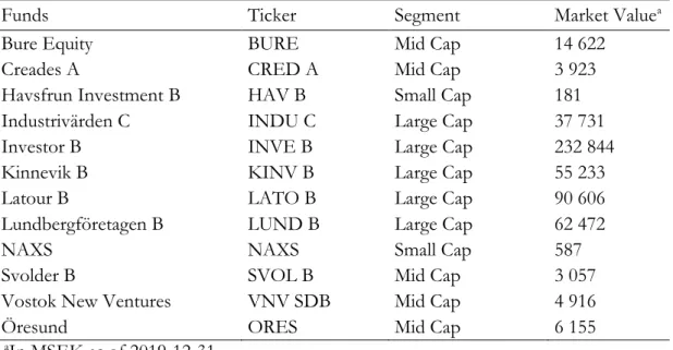
To limit the extent of the research and narrow the scope of the examination, the tests will be conducted on a selected number of funds for a specific period of time. Our sample consists of historical market prices and the self-reported net asset values of 12 Swedish CEFs cover-ing the period between Q1 2012 and Q4 2019. The selection of CEFs is based on three criteria: The company is listed on OMX Stockholm, they report their NAV themselves, and the reporting of NAV is done on an at least quarterly basis since the beginning of 2012. The reason is to make the data of the sample consistent across the CEFs by fulfilling these criteria. The data is obtained from the companies’ interim reports and price data is confirmed by checking the companies’ reported closing prices for each quarter to data from Nasdaq Nor-dic’s database for historical share prices (Nasdaq Nordic, n.d.). Closing prices are available at a daily frequency, but as the selected CEFs report their NAV quarterly, the data for both variables are collected on a quarterly basis. This is in order to have corresponding data with the same frequency for both variables. For the unit root testing later performed to answer our second hypothesis, the time span is of bigger importance than the frequency on which
the data is collected (Shiller & Perron, 1985). Similarly, in the cointegration testing for an-swering our first hypothesis, the time span is of bigger importance than the number of ob-servations. However, it should be kept in mind that for this paper’s relatively short time period, data collected on a higher frequency could give more power to the tests (Zhou, 2001). A brief overview of the sample is given in Table 3.1.
Table 3.1: Sample of CEFs
Funds Ticker Segment Market Valuea
Bure Equity BURE Mid Cap 14 622
Creades A CRED A Mid Cap 3 923
Havsfrun Investment B HAV B Small Cap 181
Industrivärden C INDU C Large Cap 37 731
Investor B INVE B Large Cap 232 844
Kinnevik B KINV B Large Cap 55 233
Latour B LATO B Large Cap 90 606
Lundbergföretagen B LUND B Large Cap 62 472
NAXS NAXS Small Cap 587
Svolder B SVOL B Mid Cap 3 057
Vostok New Ventures VNV SDB Mid Cap 4 916
Öresund ORES Mid Cap 6 155
aIn MSEK as of 2019-12-31
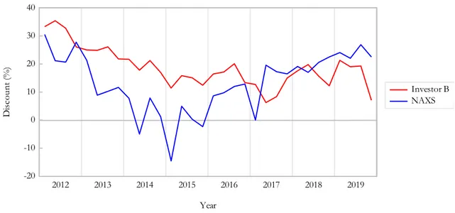
To visualize how the discount varies over time, Figure 1 compares the discount between two CEFs of different sizes, Investor B (large cap) and NAXS (small cap). It can be seen that the discount for Investor B is relatively stable for the period, with a mean of around 19 percent and range between 6 and 35 percent. This is a CEF that from a brief visualization can be observed to exhibit a mean-reverting process. In contrast, NAXS has had an initial discount of 30 percent in 2012, to then at three points in time being traded at a premium (negative discount), with a peak of a 14 percent premium in early 2015. Since then, the discount has gradually increased to a level of 23 percent at the end of 2019. The mean of NAXS’s discount is 13 percent. However, the discount is clearly more volatile than for Investor B. Conse-quently, NAXS’s discount appears to be less stable for the time-frame applied, and thus its price and NAV series ought not be cointegrated.
-20 -10 0 10 20 30 40 2012 2013 2014 2015 2016 2017 2018 2019 Investor B NAXS D is co un t ( % ) Year
Figure 1: Discount over time for Investor B and NAXS.
In fact, the discounts across the CEFs in the sample are not independent over time. In Ap-pendix Table 1, it can be seen that about half of the Pearson correlation coefficients are statistically significant at the five percent level.
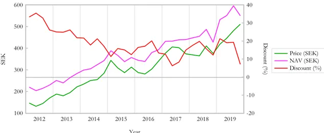
Figure 2 shows how the price and NAV move over time for Investor B, with the discount included in the same figure. Price and NAV are measured in SEK on the left axis, and the discount is measured in percent on the right axis. It can be seen that both price and NAV have clearly positive trends. From Figure 2 alone, price and NAV are perceivably non-sta-tionary, in the sense defined in Chapter 2.1.3. Furthermore, the two time series tend to move in the same direction for most periods, indicating a possible long-run equilibrium relationship between them. It illustrates the relationship between the variables and the potentially lucra-tive investment opportunities at certain times.
100 200 300 400 500 600 -20 -10 0 10 20 30 40 2012 2013 2014 2015 2016 2017 2018 2019 Price (SEK) NAV (SEK) Discount (%) SE K Year D isc ou nt (% )
Figure 2: Price, NAV and Discount for Investor B.
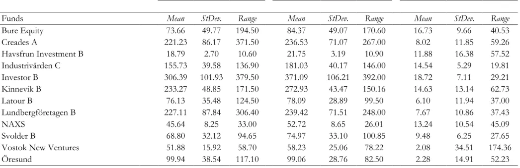
Table 3.2 presents descriptive statistics of price, NAV and discount for each of the twelve CEFs in the sample. On average, all CEFs have during the period been traded at positive discounts. The share with the highest average price is Investor B at around SEK 306, with a corresponding average NAV of about SEK 371. Investor B is also the share with the highest average discount in the sample, with a value of close to 19 percent. In contrast, the discount of Vostok New Ventures is close to two percent on average, with a large range of 174 per-cent. The discount has rapidly moved from a large premium to a more normal discount between the middle of 2013 to late 2017. Due to this extreme range in comparison to the rest of the sample, the results should be interpreted with caution. More on this in Chapter 6.
Table 3.2: Descriptive Statistics
Price (SEK) Net Asset Value (SEK) Discount (%)*
Funds Mean StDev. Range Mean StDev. Range Mean StDev. Range
Bure Equity 73.66 49.77 194.50 84.37 49.07 170.60 16.73 9.66 40.53 Creades A 221.23 86.17 371.50 236.53 71.07 267.00 8.02 11.85 59.26 Havsfrun Investment B 18.79 2.70 10.60 21.75 3.19 10.90 11.88 16.38 57.52 Industrivärden C 155.73 39.58 136.90 181.03 40.17 146.00 14.54 5.29 19.81 Investor B 306.39 101.93 379.50 371.09 106.21 392.00 18.72 7.11 29.21 Kinnevik B 233.27 48.85 171.50 272.93 43.47 150.16 14.63 13.14 62.73 Latour B 76.13 35.48 124.50 78.09 28.89 99.50 6.10 11.94 37.00 Lundbergföretagen B 227.11 87.84 306.40 239.42 71.51 248.00 7.67 10.86 37.43 NAXS 45.64 8.25 33.00 52.72 8.65 26.01 13.24 10.54 45.09 Svolder B 68.80 32.12 94.65 74.97 33.10 100.85 9.48 6.25 27.65
Vostok New Ventures 51.88 15.92 58.70 58.23 25.06 78.22 2.08 34.51 174.36
Öresund 99.94 38.54 117.10 99.06 28.76 82.50 2.28 14.91 52.23
Note: N = 32.
4. Method
The purpose of this section is to provide information regarding the methodology used to process the data and concluding the results of the statistical tests used. To strengthen the reliability of the thesis, the choices made are described and motivated. The research will be limited to examine the chosen CEFs for the time period selected in Chapter 3.
4.1 Testing process for Hypothesis 1
To answer the first hypothesis “Swedish closed-end funds’ individual prices and net asset values share the same stochastic trend”, a string of tests will be conducted. First, Fisher-type tests will be conducted to get an overall view of the nature of Swedish CEFs’ prices and NAVs. Then, unit root tests will be conducted on individual CEFs’ prices and NAVs to explore them individually. Lastly, cointegration tests will be performed to examine if there is any relationship between the CEFs’ share prices and NAVs over time.
4.1.1 Fisher-type tests
To test the hypothesis of whether Swedish closed-end funds’ individual prices and net asset values share the same stochastic trend, it is first examined if the price and NAV series hold for stationarity. As presented in the literature review, most economic time series are 𝐼(1) (Engle & Granger, 1987). Testing for individual unit roots in our finite panel data set is done through two tests suitable for our type of data proposed by Choi (2001): The Fisher-type Augmented Dickey-Fuller (ADF) test, and the Fisher-type Phillips-Perron (PP) test. The ad-vantage of the Fisher-type tests is that they have the ability to examine unit root problems for a determined variable across several time series with individual unit roots. Additionally, statistical power is increased as more data is used for calculating the test statistic, and it does so by combining the p-values of several independent tests to one conclusive panel data unit root test (Maddala & Wu, 1999). As our sample consists of 12 CEFs, the Fisher Chi-square test statistic is used:
𝑃 = −2 ∑ ln(𝑝𝑖)
𝑁
𝑖=1
, (6)
simply the individual p-values, 𝑝𝑖, which come from either individual ADF tests or individual
PP tests. Also, the test holds an advantage towards other comparable cross-sectional unit root tests as it shows the highest statistical power and is very useful for small sample sizes (Maddala & Wu, 1999). If the test statistic in Equation 6 is larger than its corresponding critical value, it can be concluded that at least one of the twelve series is stationary. Overall results for the nature of CEFs’ prices and NAVs are provided from this test.
4.1.2 ADF tests and PP tests
In order to examine the nature of prices and NAVs in greater detail for the individual CEFs, the Augmented Dickey-Fuller (1979) tests and Phillips-Perron (1988) tests are conducted on prices, NAVs, as well as the variables’ first differences to determine if the variables are both 𝐼(1) for each CEF. In this study, focus lies solely on CEFs whose prices and NAVs are both 𝐼(1), hence the outcomes from these tests decide which CEFs will be tested for cointegra-tion, to ultimately answer the first hypothesis.
4.1.3 Engle-Granger (EG) tests and ECM
With the previous tests conducted, the hypothesis of whether Swedish closed-end funds’ individual prices and net asset values share the same stochastic trend can then be answered by tests for cointegration. In addition to answering the first hypothesis by applying the Engle-Granger (EG) (1987) cointegration test, the speed at which the adjustment occurs will be tested by obtaining the error correction terms. The additional tests will only be performed on the CEFs whose price and NAV series are both concluded to be 𝐼(1), that is 𝑃𝑖𝑡~𝐼(1)
and 𝑁𝐴𝑉𝑖𝑡~𝐼(1) from the ADF and PP tests as these are prerequisites for examining
coin-tegration. The Engle-Granger (1987) test will be conducted as follows: Firstly, 𝑃𝑖𝑡 is regressed
on 𝑁𝐴𝑉𝑖𝑡 using the Ordinary Least Squares (OLS) method to obtain the residuals 𝑢𝑖𝑡, shown in Equation 7.
𝑃𝑖𝑡 = 𝛽1+ 𝛽2𝑁𝐴𝑉𝑖𝑡+ 𝑢𝑖𝑡. (7)
Then, the residuals 𝑢̂𝑖𝑡 obtained from Equation 7 are checked for stationarity by running the OLS regression in Equation 8. The t-statistic of the coefficient 𝜔̂ is compared to Engle-Granger asymptotic critical values suitable for this type of test, reported by MacKinnon (2010). Those are very close to −3.336 and −3.896, at the 5% and 1% level respectively.
∆𝑢̂𝑖𝑡−1= 𝜔𝑢̂𝑖𝑡−1 (8)
If a CEF’s price and NAV series are both 𝐼(1), and 𝜔̂ from Equation 8 is statistically differ-ent from zero, the hypothesis that a CEF’s price and NAV share the same stochastic trend is validated. Hence, there is an equilibrium relationship between price and NAV, as theory suggests. As the market price of the CEF is a representation of all information available, the price fully reflects the fund’s current assets and future cash flow according to efficient market theory (Fama, 1970). Thus, as information is provided, the adjustment will occur instantane-ously to correct for the amended information. This notion brings the momentum of the correction into the question.
As the Engle-Granger (1987) test for cointegration enlightens the long-run relationship be-tween the variables price and NAV, an Error Correction Model (ECM) is applicable to ex-amine the short-run relationship. As short-term investors make more rapid investment deci-sions, often based on technical signals, it is of importance to examine if the relationship also appears in the short-run. The ECM is an additional procedure for the cointegration test as it uses the error term collected from the EG cointegration test to determine the speed at which the variables move towards equilibrium.
Consider the long-run equilibrium as the model specified previously in Equation 7:
𝑃𝑖𝑡 = 𝛽1+𝛽2𝑁𝐴𝑉𝑖𝑡+ 𝑢𝑖𝑡. (7)
With the residuals from this model, the following error correction model can be estimated:
Δ𝑃𝑖𝑡 = 𝛼1+ 𝛼2Δ𝑁𝐴𝑉𝑖𝑡+ 𝛼3𝑢̂𝑖𝑡−1+ 𝜀𝑖𝑡, (9)
where 𝜀𝑖𝑡 represents a white noise error term. Equation 9 explains that Δ𝑃 is affected by not
only Δ𝑁𝐴𝑉, but also on the equilibrium term 𝛼3𝑢̂𝑖𝑡. Therefore, by obtaining the residual
term from Equation 9, the error-correction term can be described as:
And thus, the Engle-Granger error correction term manages to capture the adjustment to equilibrium. If the equilibrium error term does not equal zero, 𝑢̂𝑖𝑡 ≠ 0, it means that the model is out of equilibrium. The value of 𝛼̂3 in Equation 9 determines how fast the
equilib-rium will be restored. Thus, if the variable is significant, it would determine that the long-run cointegration also appears in the short run. Additionally, the coefficient of the variable would explain how long the arbitrage opportunity exists before the deviation from the average dis-count reverts.
4.1.4 Johansen tests and VECM
Stock & Watson (1993) argue that it is preferable to perform at least two tests for the objec-tive of finding cointegrating vectors. Therefore, an additional cointegration test will be per-formed in the shape of the Johansen maximum likelihood method (1988). Similar to the EG test, the Johansen test also examines the equilibrium relationship between the variables. In order to test the correlation, the following equations are used in the process:
𝑃𝑡 = 𝛿11𝑃𝑡−1+ 𝛿12𝑁𝐴𝑉𝑡−1+ 𝑒𝑃𝑡
𝑁𝐴𝑉𝑡= 𝛿21𝑃𝑡−1+ 𝛿22𝑁𝐴𝑉𝑡−1+ 𝑒𝑁𝐴𝑉𝑡.
(11) (12)
The maximum likelihood estimation process is used to test the presence of a cointegration vector between the time series price and NAV for the CEF. If a sufficient number of lags are included based on the assumption of well-behaved disturbance terms, then two investi-gation methods, the trace, 𝜆𝑡𝑟𝑎𝑐𝑒, and the maximum eigenvalue 𝜆𝑚𝑎𝑥, can be used to
deter-mine if cointegration vectors are present. The presence of one cointegration vector indicates that there is a long-run relationship between the time series. With the only two variables, price and NAV, being included, it is only possible for one vector to be present. As the test is based on the premise of 𝑟 = 𝑟∗ < 𝑘, the number of cointegration vectors and the
alter-native is 𝑟 = 𝑘 where 𝑟 represents the cointegrating rank and 𝑘 = 1. If 𝜆𝑡𝑟𝑎𝑐𝑒 or 𝜆𝑚𝑎𝑥
indicate the presence of a cointegration vector, then the solution for the two equations pro-duced becomes:
Equation 13 describes the long-term relation between price and NAV for the CEF where each column of the variable 𝜃 represents the cointegrating vector. Thus, if a cointegration vector is present then 𝜃 will equal one, meaning that price and NAV are cointegrated, i.e. they share the same stochastic trend. Thus, a conclusion can be drawn implying that the market price of the CEF and its NAV do not follow individual stochastic trends but instead share the same stochastic trend. If a deviation from the relationship of one the variables would occur it is expected that at least one of the variables ought to adjust and correct for the change in the relationship. Therefore, it is of the essence to determine which of the variables adjusts to which if it can be concluded that there is a long-run relationship. If such a finding would conclude that the price variable corrects to the NAV, the strategy of arbitra-tion investment is viable and could potentially enable the investor to achieve excess returns.
4.2 Testing Process for Hypothesis 2
To answer the second hypothesis “There is mean reversion of the NAV-discount for Swe-dish closed-end funds”, two different tests will be conducted. First, Fisher-type tests will be conducted to get an overall view of Swedish CEFs’ discounts. Then, unit root tests will be conducted on individual CEFs’ discounts to determine which ones are mean-reverting. If results from the previous tests conclude a specific CEF’s price and NAV to be cointegrated, it should follow that the discount is stationary, i.e. mean-reverting.
In a similar way of testing the first hypothesis, the Fisher-type Augmented Dickey-Fuller test and Fisher-type Phillips-Perron test are performed. However, they will be performed on the discounts. Recall that the discount is calculated as (𝑁𝐴𝑉𝑖𝑡− 𝑃𝑟𝑖𝑐𝑒𝑖𝑡)/𝑁𝐴𝑉𝑖𝑡 for CEF 𝑖 at
time 𝑡. If an individual CEF’s discount does not possess a unit root, it is stationary, and the process is mean-reverting. As argued in Chapter 1, classical financial concepts state that the price should reflect the underlying assets. The descriptive statistics show that this is not the case of CEFs. Nonetheless, the tests conducted for the CEFs’ discounts will be of im-portance to determine if there are profitable investment opportunities, based solely on dis-count movement over time.
5. Results and Analysis
In the first section of this chapter, the outcomes of the statistical tests will be presented. In the second section, the results of the tests will be interpreted and analysed in relation to the hypotheses as well as the theories and previous research they build upon.
5.1 Hypothesis 1 Statistical Findings
5.1.1 Fisher-type tests
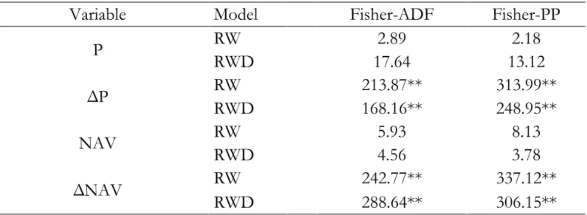
Table 5.1 reports the results from the Fisher-type tests, conducted on P and NAV, as well as their first-differences, denoted as ΔP and ΔNAV respectively. Two models are tested for each variable: a pure random walk (RW), and a random walk with drift (RWD). The tests are conducted to determine if all time series for the variables, across the twelve CEFs, possess individual unit roots. If the Fisher-Chi square test statistics are significant, at least one of the twelve CEFs' time series is stationary. The results show that both variables, price and NAV, for all twelve CEFs are nonstationary. After taking first-differences, at least one of the twelve CEFs is stationary in price and NAV.
Table 5.1: Fisher-type ADF tests and Fisher-type PP tests
Fisher Chi-square statistics
Variable Model Fisher-ADF Fisher-PP
P RW 2.89 2.18 RWD 17.64 13.12 ΔP RW 213.87** 313.99** RWD 168.16** 248.95** NAV RW 5.93 8.13 RWD 4.56 3.78 ΔNAV RW 242.77** 337.12** RWD 288.64** 306.15**
*Statistically significant at the 5% level. **Statistically significant at the 1% level. 5.1.2 ADF tests and PP tests
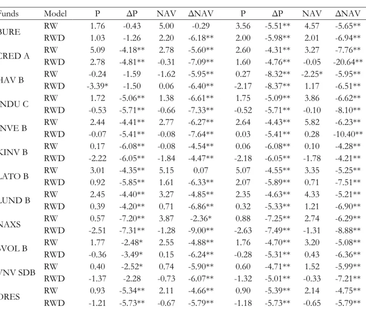
The Fisher-type tests only give a general result. In order to determine the nature of the twelve Swedish CEFs’ individual prices and NAVs, Augmented Dickey-Fuller (1979) tests and Phil-lips-Perron (1988) tests of unit root processes are conducted to determine which CEFs’ price
and NAV are 𝐼(0), or 𝐼(1) as theory suggests. Table 5.2 presents the results. The results show that for most CEFs, both P and NAV are 𝐼(1), which motivates later tests of cointe-gration. However, two out of the twelve CEF’s prices and NAVs are not 𝐼(1). For Havsfrun Investment B’s price in its RWD model, the ADF-test concludes stationarity at the five per-cent level. Also, for NAV in its RW model, the PP-test concludes stationarity at the five percent level. For Bure Equity, the ADF-tests for ΔP are insignificant, in contrast to the PP-tests that are significant at the one percent level.
Table 5.2: ADF tests and PP tests
Augmented Dickey-Fullera Phillips-Perronb
Funds Model P ΔP NAV ΔNAV P ΔP NAV ΔNAV
BURE RW 1.76 -0.43 5.00 -0.29 3.56 -5.51** 4.57 -5.65** RWD 1.03 -1.26 2.20 -6.18** 2.00 -5.98** 2.01 -6.94** CRED A RW 5.09 -4.18** 2.78 -5.60** 2.60 -4.31** 3.27 -7.76** RWD 2.78 -4.81** -0.31 -7.09** 1.60 -4.76** -0.05 -20.64** HAV B RW -0.24 -1.59 -1.62 -5.95** 0.27 -8.32** -2.25* -5.95** RWD -3.39* -1.50 0.06 -6.40** -2.17 -8.37** 1.17 -6.51** INDU C RW 1.72 -5.06** 1.38 -6.61** 1.75 -5.09** 3.86 -6.62** RWD -0.53 -5.71** -0.66 -7.33** -0.52 -5.71** -0.10 -8.10** INVE B RW 2.44 -4.41** 2.77 -6.27** 2.64 -4.43** 5.82 -6.23** RWD -0.07 -5.41** -0.08 -7.64** 0.03 -5.41** 0.28 -10.40** KINV B RW 0.17 -6.08** -0.08 -4.54** 0.06 -6.08** 0.10 -4.28** RWD -2.22 -6.05** -1.84 -4.47** -2.18 -6.05** -1.78 -4.21** LATO B RW 3.01 -4.35** 5.15 0.07 5.07 -4.55** 3.35 -5.25** RWD 0.92 -5.85** 1.61 -6.33** 2.07 -5.89** 0.71 -7.51** LUND B RW 2.45 -4.40** 3.27 -4.85** 2.35 -4.63** 4.33 -5.21** RWD 0.39 -4.20** 0.71 -6.86** 0.32 -5.33** 1.21 -6.90** NAXS RW 0.57 -7.20** 3.87 -2.36* 0.88 -7.25** 2.74 -6.29** RWD -2.51 -7.31** -1.28 -9.00** -2.63 -7.49** -1.31 -8.88** SVOL B RW 1.77 -2.48* 2.55 -4.88** 1.76 -4.70** 3.20 -5.08** RWD -0.36 -3.49* 0.15 -6.24** -0.28 -5.31** 0.43 -6.36** VNV SDB RW 0.40 -2.52* 0.74 -5.90** 0.60 -4.71** 1.52 -5.99** RWD -1.37 -2.28 -0.73 -6.07** -1.32 -5.01** -0.33 -7.21** ORES RW 0.93 -5.34** 2.11 -4.66** 0.90 -5.39** 2.14 -4.75** RWD -1.21 -5.73** -0.67 -5.79** -1.18 -5.73** -0.65 -5.79**
Note: N = 32 for each fund, before lag length selection.
aLag length is automatically selected based on the Schwarz information criterion (SIC). bBandwidth is automatically selected by Newey-West using Bartlett kernel.
5.1.3 Engle-Granger (EG) tests and ECM
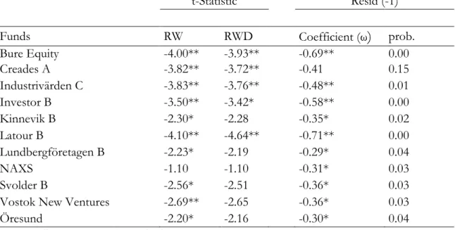
As cointegration tests require both variables to be 𝐼(1), Havsfrun Investment B will not be tested for cointegration. Even though the ADF test and PP test do not give a unanimous result regarding Bure Equity, it will still be included in further testing for cointegration be-tween price and NAV. To test for cointegration, the residuals for NAV and price obtained from the stationary time series can be tested for the presence of a unit root. The test con-cludes that if the residuals of two variables are stationary they are cointegrated and can thus be established that cointegration exists. Table 5.3 shows the results of the stationary residuals from NAV and price for each respective CEF. One can observe that all of the included CEFs except NAXS, show significant test statistics and thus show signs of cointegration. The result indicates that out of the eleven CEFs tested, there are long-run relationships between the prices and NAVs for ten CEFs. The lagged residuals represent the error correction terms which ties the long-run equilibrium to a short-run cointegration. As all of the long-run coin-tegrated funds, except for Creades A, have significant error correction terms compared to the five percent significance level, it can be concluded that the observed long-run cointegra-tion is also significant in the short-run.
Table 5.3: Unit Root Cointegration test and Error Correction Terms for residuals
t-Statistic Resid (-1)
Funds RW RWD Coefficient (ω) prob.
Bure Equity -4.00** -3.93** -0.69** 0.00 Creades A -3.82** -3.72** -0.41 0.15 Industrivärden C -3.83** -3.76** -0.48** 0.01 Investor B -3.50** -3.42* -0.58** 0.00 Kinnevik B -2.30* -2.28 -0.35* 0.02 Latour B -4.10** -4.64** -0.71** 0.00 Lundbergföretagen B -2.23* -2.19 -0.29* 0.04 NAXS -1.10 -1.10 -0.31* 0.03 Svolder B -2.56* -2.51 -0.36* 0.03
Vostok New Ventures -2.69** -2.65 -0.36* 0.03
Öresund -2.20* -2.16 -0.30* 0.04
*Statistically significant at the 5% level. **Statistically significant at the 1% level.
5.1.4 Johansen tests and VECM
For examination of cointegration using the Johansen method it is configured as the trace statistics, 𝜆𝑡𝑟𝑎𝑐𝑒, states that there are no cointegrating vectors present in the time series, 𝑟 =
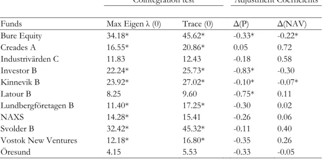
0, and must be rejected for seven out of the twelve CEFs according to Table 5.4. For the maximum eigenvalue, 𝜆𝑚𝑎𝑥, the results of the test coincide with the results of the trace sta-tistics, where the test for eight of the CEFs can be determined to include cointegrating vec-tors. The Vector Error Correction Model (VECM) is used to observe if the cointegration between NAV and Price can be tied to a short-run equilibrium. As only seven of the CEFs shows signs of long-run cointegration from the Johansen test, the vector error correction terms are only applicable to these seven funds. In Table 5.4, the test concludes that Bure Equity, Kinnevik B, and Investor B are the CEFs that can be concluded to be cointegrated for the variables of price and NAV in both a long-run and short-run perspective. The time series thus behave in a similar pattern regardless of the time frame. As the focus lies on the effect that NAV has on price, the variable Δ𝑁𝐴𝑉 is the one of importance. Here only two CEFs show significant error correction terms, 22 percent for Bure Equity and 7 percent for Kinnevik B. This implies that it will be the price that adjusts for an equilibrium deviation. These variables can be interpreted as the speed of adjustment for the previous periods’ de-viation from long-run equilibrium. The variable of Δ𝑃 is included in the table for the purpose to be able to relate to previous research as that variable has been chosen to be included.
Table 5.4: Johansen Cointegration test and Vector Error Correction Terms
Cointegration test Adjustment Coefficients
Funds Max Eigen λ (0) Trace (0) Δ(P) Δ(NAV)
Bure Equity 34.18* 45.62* -0.33* -0.22* Creades A 16.55* 20.86* 0.05 0.72 Industrivärden C 11.83 12.43 -0.18 0.58 Investor B 22.24* 25.73* -0.83* -0.30 Kinnevik B 23.92* 27.02* -0.10* -0.07* Latour B 8.25 9.60 -0.75* 0.11 Lundbergföretagen B 11.40* 17.25* -0.30 0.02 NAXS 14.28* 15.41 -0.26 0.06 Svolder B 32.42* 45.32* -0.11 0.40
5.2 Hypothesis 2 Statistical Findings
5.2.1 Fisher-type tests
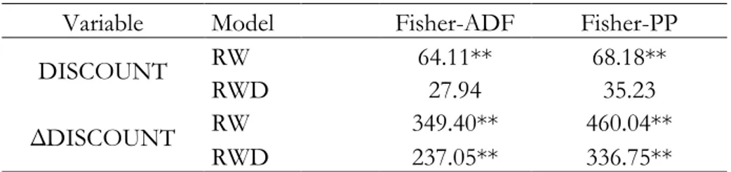
The results obtained to answer the hypothesis whether there is mean reversion of the NAV-discount for Swedish closed-end funds are presented in Table 5.5 and Table 5.6. Table 5.5 presents the results for the Fisher-type tests conducted on the CEFs’ discounts. Because the discount is statistically significant at the one percent level in the random walk model for both tests, it can be concluded that at least one of the twelve CEFs’ discount is mean-reverting. This is in line with the cointegration results, and previous studies that show mean-reverting discounts among CEFs.
Table 5.5: Fisher-type ADF tests and Fisher-type PP tests
Fisher Chi-square statistics Variable Model Fisher-ADF Fisher-PP
DISCOUNT RW 64.11** 68.18**
RWD 27.94 35.23
ΔDISCOUNT RW 349.40** 460.04**
RWD 237.05** 336.75**
*Statistically significant at the 5% level. **Statistically significant at the 1% level.
5.2.2 ADF tests and PP tests
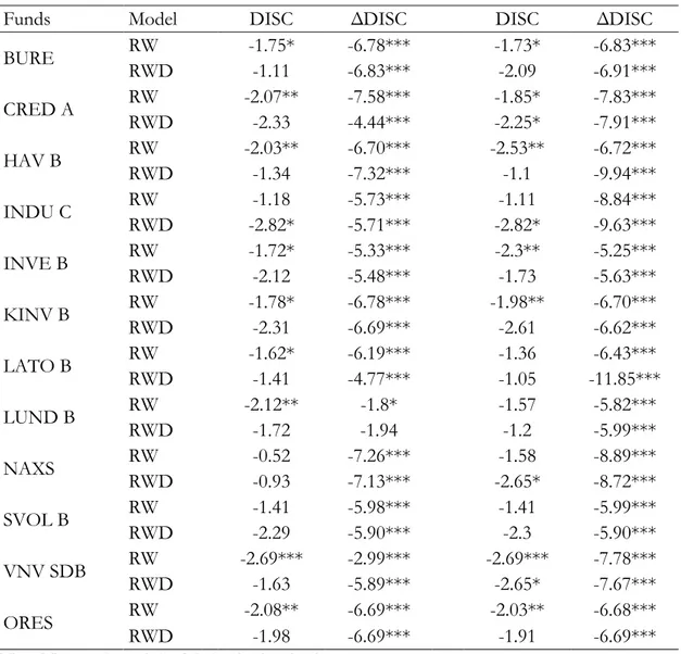
To attain results on a fund specific level, Augmented Dickey-Fuller tests and Phillips-Perron tests are shown in Table 5.6. The ADF test for discount reveals that nine out of twelve Swedish CEFs’ discounts are mean-reverting (RW), while the PP test shows that seven out of twelve Swedish CEFs’ discounts are mean-reverting (RW). Hence, timely investments where an investor enters when the discount is relatively large, and exits when the discount has narrowed, can be profitable in some Swedish CEFs. Important to note is that they are significant at the ten percent level of significance. From the data used, it can, therefore, be stated that there are signs of mean reversion of the NAV-discount for some of the Swedish closed-end funds as hypothesis two states.
Table 5.6: Unit root tests for discount
Augmented Dickey-Fullera Phillips-Perronb
Funds Model DISC ΔDISC DISC ΔDISC
BURE RW -1.75* -6.78*** -1.73* -6.83*** RWD -1.11 -6.83*** -2.09 -6.91*** CRED A RW -2.07** -7.58*** -1.85* -7.83*** RWD -2.33 -4.44*** -2.25* -7.91*** HAV B RW -2.03** -6.70*** -2.53** -6.72*** RWD -1.34 -7.32*** -1.1 -9.94*** INDU C RW -1.18 -5.73*** -1.11 -8.84*** RWD -2.82* -5.71*** -2.82* -9.63*** INVE B RW -1.72* -5.33*** -2.3** -5.25*** RWD -2.12 -5.48*** -1.73 -5.63*** KINV B RW -1.78* -6.78*** -1.98** -6.70*** RWD -2.31 -6.69*** -2.61 -6.62*** LATO B RW -1.62* -6.19*** -1.36 -6.43*** RWD -1.41 -4.77*** -1.05 -11.85*** LUND B RW -2.12** -1.8* -1.57 -5.82*** RWD -1.72 -1.94 -1.2 -5.99*** NAXS RW -0.52 -7.26*** -1.58 -8.89*** RWD -0.93 -7.13*** -2.65* -8.72*** SVOL B RW -1.41 -5.98*** -1.41 -5.99*** RWD -2.29 -5.90*** -2.3 -5.90*** VNV SDB RW -2.69*** -2.99*** -2.69*** -7.78*** RWD -1.63 -5.89*** -2.65* -7.67*** ORES RW -2.08** -6.69*** -2.03** -6.68*** RWD -1.98 -6.69*** -1.91 -6.69***
Note: N = 32 for each fund, before lag length selection.
aLag length is automatically selected based on the Schwarz information criterion (SIC). bBandwidth is automatically selected by Newey-West using Bartlett kernel.
*Statistically significant at the 10% level. **Statistically significant at the 5% level. ***Statistically significant at the 1% level.
5.3 Analysis
As the purpose of the thesis was set out to examine two questions; whether or not the price and NAV for Swedish CEFs share the same stochastic trend, and two; if the NAV-discount is mean-reverting over time. The questions were examined through a string of statistical tests. The order of the tests was organized as first determining which of the selected CEFs have
stationary time series for both their price and NAV. According to Table 5.2, it can be con-cluded that out of the twelve funds, only Havsfrun Investment B, shows no sign of station-arity for both the variables after taking first differences. This result is in line with the notion that many economic time series are nonstationary, well documented by Poterba and Sum-mers (1988). Stationarity of at least the first difference is a prerequisite for further testing of cointegration and Havsfrun Investment B must therefore be excluded in any further statisti-cal testing for cointegration.
To further examine the hypothesis, two cointegration tests were performed. Table 5.3 shows that the results from the Engle-Granger two-step approach indicate that ten out of the eleven included funds’ price and NAV appears to be cointegrated. The results can be interpreted as the two time series share a common stochastic trend meaning that they tend to move towards a long-run equilibrium, a sign that strengthens the hypothesis of cointegration between a CEF’s NAV and price as the two time series can be concluded to revolve around the same stochastic trend. The results coincide with what the efficient market theory suggests, which according to Fama (1970), means that the share price should reflect the available information at that given point in time. It should therefore capture the publicly accessible information regarding the fund’s underlying assets and thus follow the net asset value of the fund.
To strengthen the findings of the cointegration test, the Johansen method was used to ex-amine the presence of cointegrating vectors. Table 5.4 shows that seven and eight of the included funds have a cointegrating vector for the trace test and maximum eigen test respec-tively. Despite the fact that most of the funds indicate cointegration between the variables, there is no sweeping evidence of cointegration for all of the CEFs. Instead, it can be con-cluded that the evidence of cointegration between the NAV and price for a CEF varies amongst the individual funds and must therefore be examined on a fund specific basis. The result for some of the funds is contradicting to that of the Engle-Granger test which can make the result doubtful. The reason being is most likely due to a small sample size and therefore lowers the power of the cointegration tests. The problem and its consequences will be further assessed in Chapter 6. The tests show opposing results to the previous research of Gasbarro et al. (2003) as they conclude that the Johansen method gives a result of more funds that shows signs of cointegration between the two variables and fewer funds when using the Engle-Granger method.
To determine if the cointegration not only appears in the long-run but in the short-run as well, the error correction terms are observed in both methods. From the Engle-Granger method, it can be determined that eight of the nine CEFs that showed signs of a long-run relationship also indicates a short-run relationship. The results state that the two variables move in a correlated pattern. This creates a window of opportunity for investors if the dis-crepancy between the market price and the NAV increases as it statistically shows that for the chosen CEFs the gap will most likely narrow. Important to bear in mind is that there are two ways for the discount deviation to close, either for the price to increase, or the NAV to decrease. As it will only profitable for investors if the price increase, it will be of the essence to determine which of the variables that adjusts to reestablish the equilibrium. That can be determined by the help of the vector error correction term of the Johansen method.
As seven of the funds in the Johansen method rejects the notion of no cointegration for both the max-eigen and trace statistics, as presented in Table 5.4, the vector error correction terms are only viable for these funds. Out of those seven funds, there is only Bure Equity, Investor B, and Kinnevik B who portray significant vector error correction terms. The result indicates that there is a short-run cointegration between the funds’ prices and NAVs. As previously mentioned, this enables for a profitable opportunity for an investor if and only if it can be concluded that it is the price that adjusts to the equilibrium and not the NAV. Therefore, the variable Δ𝑁𝐴𝑉 is the important variable as it normalises price and can there-fore be used in determining if it is the price that is the adjusting variable. This can only be determined for Bure Equity and Kinnevik B as all other funds fail to show significant vector error correction terms.
For answering the second hypothesis of mean reversion of the NAV-discount for Swedish closed-end funds the results of the tests presented in Table 5.5 and Table 5.6 suggest that the discount of the chosen CEFs appears to mean revert. The finding coincides to the earlier research of Poterba and Summers (1988) who state that share price shows no indication of independent movements depending on a few characteristics. Gasbarro et al. (2003) also con-clude in their extensive research of mean-reverting characteristics for American bond and equity CEFs’ discounts. Furthermore, the result coincides with the studies by Malkiel (1995), Thompson (1978) and Pontiff (1997) suggesting that the discount tends to move in a revert-ing pattern to restore the historical mean. The compelled findrevert-ings suggest that the observed
movement in the discount variable allows for excess returns as an arbitrage opportunity ap-pears when the discount is historically large. However, it is important to note that there can be no general conclusion drawn from the research as the movement is fund specific depend-ing on a number of characteristics and not applicable to the general mass of CEFs. What can be said is that profitable trading opportunities based on the discount alone do exist for certain Swedish CEFs.
Our research finds that Bure Equity is one of the CEFs that shows statistical evidence of mean-reversion in the discount. In fact, 81 percent of Bure Equity’s holdings are listed assets (2019). Information regarding the valuation of the underlying assets would therefore be easily obtained compared to if instead the fund would by a majority consist of non-securitized assets leading the investor to make more assumptions for valuing the fund based on its NAV. Also, the discount of Öresund has been concluded to be mean-reverting at the 5 percent level of significance. Similar to Bure Equity, its fraction of listed holdings to total holdings is large, at 92 percent (2019). On the other hand, Vostok New Ventures, the only CEF whose discount appears to be mean-reverting at the 1 percent significance level, exclusively invests in non-listed companies (2019). Hence from this paper, no conclusions can be drawn regard-ing the relationship between the fraction of listed underlyregard-ing assets and the discount.
6. Discussion and Conclusion
In accordance with the opinion of Stock & Watson (1993), it is favourable to perform more than one test when testing the presence of cointegrating vectors. The argument provided motivates the choice made of performing both the Engle-Granger two-step cointegration test as well as the Johansen maximum likelihood method. Noticeably, the results of the coin-tegration tests between the two variables differ for the two tests for specific funds. However, the results are coinciding on a more general level where the clear majority of the CEFs indi-cate evidence of cointegrating vectors.
Another topic we believe to be important to shed light upon is the data used in the testing process. The data consists of quarterly data ranging from the period of Q1 2012 to Q4 2019, consisting of 32 observations for each variable for the sample of CEFs. The drawback of the Phillips-Perron test to the Augmented Dickey-Fuller test is that since it is based on asymp-totic theory, it is problematic in small sample sizes, as in our case (Maddala & Wu, 1999). This motivates the reason for performing the Fisher-type test as it is able to combine the data for all twelve funds, thus, the sample size becomes sufficiently large with n=384. How-ever, Shiller and Perron (1985) argue that the statistical power of the test is more dependent on the time span of the data rather than the included number of observations. Thus, causing concern for the significance of our results as the span of the data collected only covers a period of eight years in total. Important to bear in mind is that the period between 2012 and 2019 remarks as a strong period of economic activity for the Swedish economy. The result may therefore very likely be time-dependent and only consistent for the period chosen. To provide stronger evidence for the hypothesis of mean reversion in the net asset value dis-count for Swedish CEFs, a longer period of time is necessary.
The observant reader notices that the range in the discount variable for Vostok New Ven-tures is close to 175 percent as presented in Table 3.2. Yet, the Augmented Dickey-Fuller test concludes that the variable is stationary at the one percent level of significance. The reason being for this seemingly contradictory result is that Vostok New Ventures has two outliers in their data samples at the beginning of the time period. Therefore, the range of the discount variable becomes substantially larger than expected. Adjusting for these two outli-ers, the range instead becomes 69 percent, an interval much more consistent with the result of the test. The reason for such a divergence to occur is most likely explained by the structure