Forest Cover and Economic Development : A cross-country study on the relationship between forest cover and economic development in South America

Forest Cover and Economic Development

A cross-country study on the relationship between forest cover and

economic development in South America

BACHELOR THESIS WITHIN: Economics NUMBER OF CREDITS: 15

PROGRAMME OF STUDY: International Economics AUTHOR: Terry Dalberg & Felix Svensson

i

Acknowledgements

We, Terry Dalberg and Felix Svensson, would like to take this opportunity to express our gratitude to a couple of people who have supported us throughout the hard work of this thesis.

We would like to show our gratitude to our supervisor, Anna Nordén, for her constructive criticism, irreplaceable guidance and all of her many advice during the writing of this thesis. Without her guidance and pedagogical teaching in how to conduct a thesis, this would not be possible.

Also, we are very thankful for all the help and inputs for which we have received from our classmates during the seminar sessions.

Thank you!

Jönköping International Business School May 2021

ii

Bachelor Thesis in Economics

Title: Forest Cover and Economic Development Authors: Terry Dalberg and Felix Svensson

Tutor: Anna Nordén Date: Spring 2021

Key terms: Deforestation, share of land covered by forest, Environmental Kuznets Curve for Deforestation, Forest Transition Theory, South America, Economic Development

Abstract

Ongoing deforestation is an urgent, global issue with both direct and indirect impacts on a nation’s future development. This as change in forest cover and economic development provides an intuitive link between each other. Deforestation is driven by the expectations of economic return through exploitation of natural resources in search for economic

development. The purpose of this paper is to investigate the relationship between change in forest cover and economic development in South America between 1991 and 2019. Even if deforestation is considered widely studied, it remains an empirical question how it relates to economic development. This study uses the framework of Environmental Kuznets Curve for Deforestation (EKCD), an economic theory which suggest that economic development has an

inverted U-shaped relationship with deforestation. By using a fixed effect model, we find evidence of a U-shaped relationship between forest cover and income (GDP per capita). Our results indicate that a country’s forest cover decline as income raises until a turning point is reached, after which forest cover increases together with advancing economic development. Hence, provide empirical evidence of the existence of a U-shaped EKCD in South America.

Furthermore, the study is conducted using average data and the turning point therefore is also an average for the continent.

iii

Table of Contents

1.

Introduction ... 1

2.

Theoretical frameworks and Empirical Evidence ... 5

2.1 Forest Transition Theory ... 5

2.2 Environmental Kuznets Curve for Deforestation Theory ... 7

2.3 Previous Empirical Results ... 9

2.4 Drivers of Deforestation ... 13

2.5 Hypothesis ... 14

3.

Econometric Method and Data ... 15

3.1 Econometric Method ... 15 3.2 Turning Point ... 17 3.3 Data ... 17

4.

Results ... 19

5.

Discussion ... 24

6.

Conclusion... 27

Reference list ... 29

Appendix ... 34

iv

Figures

Figure 1 - Change in (%) Share of land covered by forest ... 1

Figure 2 - Forest Transition Theory ... 6

Figure 3 - Environmental Kuznets Curve - Deforestation ... 8

Figure 4 - Economic Development ... 22

Tables

Table 2 - Descriptive Statistics ... 19

Table 3 - Covariance Matrix ... 19

Table 4 - The relationship between Forest cover and GPD per capita ... 21

Appendix

Appendix 2 - Cointegration test ... 36

Appendix 3 - Lagrange and Hausman test ... 36

Appendix 4 - Serial Correlation test ... 37

1

1. Introduction

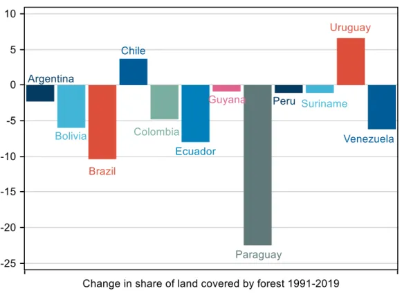
Deforestation is considered the second largest anthropogenic source of carbon dioxide to the atmosphere (Song et al., 2015).  37 percent of the world’s tropical forests are found in South America, and thus deforestation within the continent is a large contributor to the loss in tropical forest and has continued to take place at alarming rates (Benhin, 2006). Forest in South America provides livelihood and nourishment for millions of people, thus the decline in forest cover can be devastating for millions of people. Between the years of 1990-2019 all countries in South America except Chile and Uruguay have been facing a decline in share of land covered by forest, i.e., experienced deforestation, see Figure 1.

Figure 1 - Change in (%) Share of land covered by forest

Deforestation is often driven by the anticipation of economic return as a result of countries exploiting their natural resources to seek for economic development (Renoir & Guttentag, 2018). Expansion of agriculture land is one of the main drivers of deforestation in South

2

America. In Argentina mainly due to soybean production (Grau, Gasparri, Mitchell Aide, 2004) and in the Bolivian and Brazilian Amazon due to the expansion of cattle ranching and soybean farming (Mena, Bilsborrow, & McClain 2006; Ometto, Dutra Aguiar, & Martinelli, 2014). Deforestation affects the long-term possibility to grow, as well as contribute to climate change, decrease biodiversity and human wellbeing, which gives importance to investigating the relationship between deforestation and economic development. Underlying drivers of deforestation mentioned in the literature involves increase in overall population, shifting in agricultural trade and impacts from socio-political institutions (Scrieciu, 2007).

According to the theory of Environmental Kuznets Curve (EKC) the deforestation trend follows a U-shaped relationship where at low level of income deforestation increases and when countries have reached a certain income level, the deforestation rate starts to decrease (Cole & Rayner, 1997). Even if the EKC for deforestation is suggested to be an anchor when explaining the forest transition approach (e.g., Barbier et al., 2010; Rudel, 2005; Mather, 1992), various studies are discontented with current literature on EKC for deforestation and calls for additional research (e.g., Chowdhury & Moran 2012). South America is interesting as it is home to the Amazon rainforest, as well as the Gran Chaco. The latter is a semi forested high temperature area spanning over Argentina, Bolivia, Paraguay and Brazil and have a high biodiversity and a rich nature life. Half of the world’s deforestation occurs within the continent of South America, where Brazil, Peru, and Bolivia accounting for 70% of the continent’s deforestation (FAO & UNEP, 2020). According to Bhattacharyya and Hodler (2010) developing countries with large amounts of natural resources tend to be more corrupt, since there might not be sound institutions to keep the government accountable. Overall, South America have issues with corruption, and this can lead to lack of enforcement or skipping of the regulations in place to harvest more forest than sustainable to create higher profits (Global Corruption report, 2011)

Prior research regarding changes in forest cover have focused on Latin America (Barbier & Burgess, 2001; Bhattarai & Hammig, 2001; Cropper & Griffiths, 1994) which makes it hard to disentangle the effect on forest cover in South America. Many have extensively studied changes in forest cover on both a national and regional level (Hansen, 2013; Velasco Gomez, 2015). All of which have found some evidence for the EKC for deforestation. However, focus has rather been on carbon losses (Achard, 2002; Hansen, 2008) than economic drivers of deforestation

3

(Renoir & Guttentag, 2018). Between the years of 1992-2012 there were 600 estimations published on the topic of EKC for deforestation. More than half of these do not corroborate its existence and has been proven elusive depending on methods, dataset and sample used which have motivated authors to criticize the theory (Choumert, Dakpo, & Motel, 2012). Despite this abundance of empirical findings, researchers find it difficult to suggest complete recommendations arising from the relationship between economic development and deforestation, thus calls for further studies. Hence, the relationship between deforestation and economic development is still in question and should be discussed more thoroughly with factors affecting both direct and indirect.

The aim of this study is to add to the literature by exploring the EKC for deforestation, i.e., the relationship between income (GDP per capita) and change in forest cover in South America. The focus in this paper is South America, a continent with large areas of tropical forests as well as socio-political instabilities affecting forests both direct as well as indirect. The complexity of a single continent as well as the lack of studies solely focusing on South America, makes this paper a contributes to the EKC for deforestation literature. This study uses forest cover data from Food and Agriculture Organization (FAO) and GDP per capita from The World Bank covering all countries in South America from 1991-2019. The relationship between deforestation and economic development are essential in the long run since an adequate economic development is very much dependent on forest as an important role in providing ecosystem services, biodiversity and human wellbeing. To identify the relationship between economic growth and change in forest cover we follow previous literature and use a fixed effect model (Culas, 2007). Our results show a U-shape relationship between economic growth and change in forest cover. We conclude that for South America there seems to be some evidence for the EKC for deforestation.

The thesis is structured as follows: section two presents the theoretical frameworks behind the connection between economic development and deforestation, as well as the economic drivers of deforestation and previous research within the Environmental Kuznets Curve for deforestation. Section three covers the selected method and how we build our model, this includes test for stationarity consolidated with test for autocorrelation. Section four represents our empirical findings and section five discusses our findings. In the last section we present the

4

conclusion of our research, followed by a list of references and an Appendix where data is presented in detail.

5

2. Theoretical frameworks and Empirical

Evidence

The connection between development and deforestation can be connected to two broad theoretical frameworks, the Forest Transition Theory (FTT) and Environmental Kuznets Curve for Deforestation (EKCD). FTT shed light on explaining the development faces of a country in

general and what affect it has on forest cover in these specific stages. Whereas the EKCD

explicitly targeting the relation between economic development (henceforth, GDP per capita) and deforestation rate. These two theories provide a strong theoretical framework for our study and will be thoroughly explained during this section.

2.1 Forest Transition Theory

The FTT, originally introduced by Mather (1992), argues that; in the early stage of nation development process, it is fatal for humans to use their natural resources. This will then cause a rise in price and demand of such natural commodities hence leading to more deforestation. The FTT focuses on the change in forest cover over time and when it shifts from deforestation to reforestation (Lambin & Meyfroidt, 2010). There are two main reasons to why countries cut down forests. One is the need for resources that trees provides – the wood for building materials, fuel, or paper. The second is the basic need for land usage for other types of land use such as agriculture (i.e., growing crops or pasture to raise livestock), infrastructure and urban development. As population starts to grow and countries develops the overall wealth increases hence the incentive to cut down trees will at first expand but later decline (Mather, 1999).

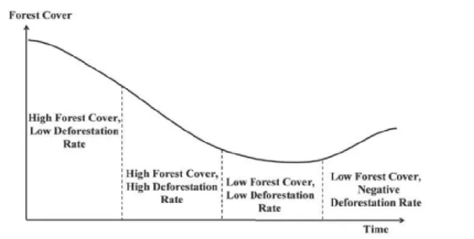
The FTT is illustrated in Figure 2. The different stages are:

Stage 1 – The Pre-Transition phase is defined as having high forest cover and very moderate losses over time.

Steg 2 – The Early Transition phase is when a country starts to lose its forest cover swiftly hence deforestation rate is high.

6

Stage 3 – The Late Transition phase occurs at the point in time when deforestation rates start to slow down again. At this moment, countries are still losing forest each year but at a slower pace. Starting to transit towards the “transition point”.

Stage 4 – The Post-Transition phase takes place when countries have progressed the transition point and are now facing afforestation again. In start of this phase, the area of forests has surpassed its lowest point. While increasing forest area the annual change in forest cover is now positive hence having a negative deforestation rate.

Figure 2 - Forest Transition Theory

Source: From Angelsen Realising REDD+ National Strategy and Policy Options (2009) page 4

The FTT have been applied by several studies to analyze land use and forest cover (e, g. Yeo & Huang 2013; Bae, Won Joo, & Kim, 2012; Müller et al., 2011). All have used the FTT as an approach to explain the importance of forest cover and deforestation over time. Yeo and Huang (2013) found evidence for the FTT in two cycles in Mississippi where in the first FTT cycle the forest cover decreased over time until reforestation occurred by reverting agricultural land to forest. During the second cycle in Mississippi the reason for reforestation, was due to decrease in population in rural areas and need for timber within the industry sector. As well as technological improvements which lead to an increased concentration of agriculture and

7

governmental improvements of forest management. Bae, Won Joo and Kim (2012) provides evidence that the FTT holds for South Korea due to the role of the government that set out a clear aim and incentivized reforestation to gain publics support for their policies and are experiencing a U-shaped curve.

One could compare this to the well-known Environmental Kuznets Curve for deforestation (EKCD) and see its similarities. While FTT breaks into four stages and is explained by the

amount of forest cover in a region over time and as forest cover first decrease and later increase it will follow a U-shaped curve (see Figure 2). The FTT is explaining the development faces of a country or a region and what affect it has on the forest in these specific development faces, rather than the EKCD that focuses explicitly on connection between economic development and

deforestation. As EKCD focuses on deforestation rate it will, contrary to the FTT, appear as an

inverted U-shape.

2.2 Environmental Kuznets Curve for Deforestation Theory

One of the most influential theory connecting economic development and environmental degradation is the Environmental Kuznets Curve (EKC). The EKC implies that a country starts from a low level of income per capita, and as income raises environmental degradation increases. This occur since, in early stage of development focus is on increasing economic growth and rising people out of poverty rather than conserving the environment. When people have problems meeting basic needs, the environment are not a top priority but rather economic growth to raise living standards. When the income has reached a certain level people will value the environment higher and more regulation will be in place as instant growth is not as equally necessary. This will result in a gradually decline of environmental degradation. This pattern results in an inverted U-shaped curve where environmental degradation increases with increased income until a turning point where increased income results in decreased environmental degradation (Dinda, 2004).

8

The EKC is originally adopted from the curve proposed by Kuznets (1955) who investigated the correlation between income and equality (the Kuznets Curve).1The EKC has later been developed and applied in the forestry sector, known as the EKC for deforestation (EKCD). This

concept was first discussed and argued for by López (1994) who proposed that as income is rising deforestation will decline. López (1994) concludes that EKCD should be an inverted

U-shaped curve as the result of the relationship between income and deforestation (see Figure 3). Diving further into the concept, theory suggest that in an early stage of development when the level of GDP per capita is relatively low, an increase in GDP per capita will increase deforestation. According to Culas (2012), as GDP per capita increase people would feel incentivized to improve their resources of forest and their environmental quality which results in a turning point and the inverted U-shaped EKCD. In this study, we use share of land covered

by forest within the EKCD framework thus we investigate if there is a U-shaped EKCD much

like the FTT rather than an inverted U-shape that is the result in an EKCD.

Figure 3 - Environmental Kuznets Curve - Deforestation

Source; From Culas Ecological Economics 79 (2012) page 46

1 _{The Kuznets curve shows an inverted U-curve between inequality (i.e., the Gini-coefficient)}

9

2.3 Previous Empirical Results

There are several well-acknowledged empirical studies on EKCD. The main underlying factors

for the change in forest cover has been found to be economic development and population growth. In this paper, we focus on research provided within Latin America, however, there is vast literature on the EKCD that shed light on Asia and Africa as well. A summary of the

estimated model(s) and evidence in the existence of EKCD used in previous empirical results

can be seen in Table 1 below.

Bhattarai and Hammig (2001) provide evidence of a relationship between deforestation and income across the Latin America and Asian continent. They use cross national analysis using panel data. This gives the researchers an increase in degrees of freedom, large number of data points which is reducing collinearity among the explanatory variables. The authors used a fixed-effect model (FEM) for which they argue is more appropriate than Pooled OLS or random fixed-effect model (REM) in this type of cross-country sample analysis. They argue that an increase in forest cover is depending more on building up a strong socio-political institution rather than factors regard macro economy and population (Bhattarai & Hammig, 2001). The same argument is made by Atmadja and Sills (2015) where they argue that developing countries face trouble with deforestation partly due to political ruling, lack of strength and willingness to deal with the issue from political and institutional point of view.

A cross-country analysis was set up by Barbier and Burgees (2001) where they covered change in forest area in 90 tropical countries in Africa, Latin America and Asia from 1961 to 1994. Results from a FEM show no significant relationship between income and forest cover in Africa and Latin America. However, a significant relationship was found for Asia. When instead conducting an OLS and adding institutional variables such as security of ownership or property rights, political stability and “rule of law”. The result changed and Latin America instead is the only region were a significant relationship is found and they estimated the turning point to be USD 6600 for Latin America. Barbier and Burgess (2001) argues that an increase in population have a negative effect on forest cover, however as a nation develops a higher GDP per capita have a positive effect on forest cover and that these mechanisms work simultaneously. They argue that a rise in GDP per capita reduces the demand for converting forests to agriculture plots. Cropper and Griffiths (1994) finds strong empirical evidence for an EKCD between the

10

years of 1961-1988 in Africa and Latin America. Using a FEM combined with Prain-Winstein technique to correct for autocorrelation they identified the turning points for GDP per capita to be USD 4760 for Africa and USD 5420 for Latin America. As a reason for deforestation they argue that population pressure is an important cause, however as argued by Culas (2007) that population increase will both increase the rate of deforestation but could also lead to innovation, technological progress and thus reduced rates of deforestation.

However, the general consensus is that an increase in population will lead to increased deforestation (Culas 2007). More recent studies are for instance a cross-country study on six countries in South America made by Ceddia, Bardsley, Gomez-y-Paloma and Sedlacek (2014) where they are using FAO data between 1970-2007. They did find significant evidence of income effect on deforestation, although, the main focus during their study is governance and agricultural effects. Culas (2007) as well as Koop and Tole (1999) both provides evidence of an inverted U-shaped EKCD in Latin America, Asia and Africa, focusing on deforestation rate

as dependent variable and explanatory variables such as agricultural production index, export price index and debt as percentage of GDP.

Explanatory variables are chosen due to the authors beliefs that they are hypothesized to affect the relationship between income and deforestation (i.e., the EKCD). Panel data method is used

with involvement of both time series and cross-sectional data. FEM as well as pooled OLS is used to estimate their parameter values, for a summary of which model is used, please see Table 1 below. Culas (2007) also corrects for auto correlation (AR1) using Cochrane-Orcutt2 transformation procedure including the generalized least squared method. Both papers found evidence of an inverted U-shaped EKCD for Latin America however Culas (2007) does not

calculate the turning point, Koop and Tole (2007) obtained a turning point at USD 8660 for Latin America.

Papers for which do not find existence of EKCD are also present. Van Nguyen and Azomahou

(2007) have done their research in the role of heterogeneity in the deforestation process and provides no evidence of an EKC for deforestation. They focus on 59 developing countries in Latin America, Africa and Asia during 1972-1994 using a panel data set. This is based on that

2 _{Cochrane-Orcutt transformation procedure is a procedure in econometrics for which it}

11

deforestation is primarily a problem in developing countries (Cropper & Griffiths, 1994) as well as most previous studies have examined developing countries, allowing them to compare their results with existing literature (Van Nguyen & Azomahou, 2007). Van Nguyen and Azomahou (2007) conduct their study by starting with a simple parametric model with deforestation rate as a dependent variable explained by economic growth (i.,e GDP per capita). The authors continue by adding explanatory variables such as population density, political institutions function and education. They conduct a Hausman test to decide if they should proceed their study with a FEM or a REM. Additionally, they find evidence for a REM, however,t they decide to follow previous literature and thus using FEM to estimate their parameters as this estimation is more suitable for a cross-country study.

The reason this study is conducted in only South America is due to the fact that the continent as a whole is not a homogenous group of countries and in different stages of development. It is also home to the largest tropical forest in the world crossing borders and are present in 8 countries within the continent and home to the greatest biodiversity on the planet. South America has lost share of land covered by forest in a great majority of the countries (see Figure 1). During a meta-analysis of the extensive research made on EKCD theory, Choumert, Dakpo

and Motel (2012) investigates the prevalence of choices made by researches (i.e., deforestation measure, econometric strategy, geographical area and measure of economic development). They investigate 71 studies, presenting over 600 estimation and shed light on the different results of EKCD where more than half do not provide evidence for the existence of an EKCD.

The authors conclude that the EKCD is disputed and will continue to be so, until stronger

empirical evidence is presented on either side. The literature on the EKCD is extensive but the

results differ over different datasets, years and methods. We want to contribute to the literature by providing more empirical evidence that is needed within the EKCD framework. This study

brings more recent data and connect our research to economic drivers as well as drivers for deforestation explaining the connection between the loss in forest cover and economic development.

12

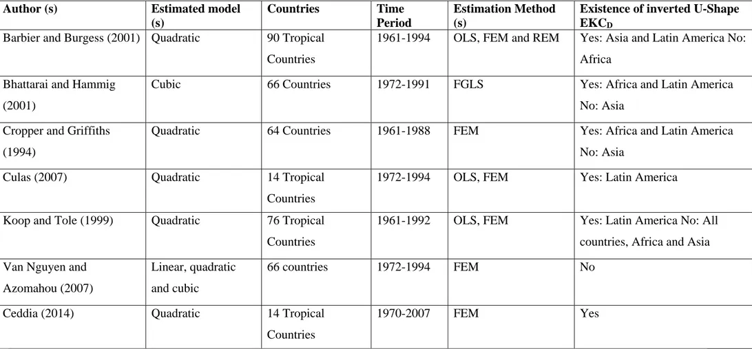
Table 1 - Previous Empirical Results

Author (s) Estimated model

(s)

Countries Time

Period

Estimation Method (s)

Existence of inverted U-Shape

EKCD

Barbier and Burgess (2001) Quadratic 90 Tropical Countries

1961-1994 OLS, FEM and REM Yes: Asia and Latin America No: Africa

Bhattarai and Hammig (2001)

Cubic 66 Countries 1972-1991 FGLS Yes: Africa and Latin America

No: Asia Cropper and Griffiths

(1994)

Quadratic 64 Countries 1961-1988 FEM Yes: Africa and Latin America

No: Asia

Culas (2007) Quadratic 14 Tropical

Countries

1972-1994 OLS, FEM Yes: Latin America

Koop and Tole (1999) Quadratic 76 Tropical Countries

1961-1992 OLS, FEM Yes: Latin America No: All countries, Africa and Asia Van Nguyen and

Azomahou (2007)

Linear, quadratic and cubic

66 countries 1972-1994 FEM No

Ceddia (2014) Quadratic 14 Tropical

Countries

1970-2007 FEM Yes

* Note: OLS, Ordinary Least Squares. FEM, fixed-effect model. REM, random-effect model. FGLS, feasible generalized least squares

13

2.4 Drivers of Deforestation

The empirical literature is ambiguous in the existence of an EKCD. Some studies have

found a U-shaped relationship between forest cover and economic development (Bhattarai & Hammig, 2001; Culas, 2007) while others have not (Van Nguyen & Azomahou, 2007). There are several drivers of deforestation that could explain this ambiguity. One explanation to the turning point of the EKCD is that as a country becomes

wealthier it enables a development of a better forest management and build awareness for forest conservation (Angelsen, 2009). Furthermore, institutional, and socio-political instabilities can have biased incentives towards lands use which lead to cumulative deforestation trends, which in the long run delays onset of forest transition. Such distortions have a major impact, as drivers of deforestation, in prolonging the forest cover loss (Burgess et al., 2011). In South America many nations are considered developing tropical economies with many social-political instabilities.

Comprehensive drivers of deforestation are urbanization and change in population. According to the Boserup effect an increase in urban population leads to more creativity and increased use of technology in the agriculture sector which put less pressure on forests (Boserup, 1970). The argument made is that with improved technology the need to expand agricultural land is decreasing since the productivity of existing land increases. As mentioned previously expansion of agricultural land is one of the main drivers of deforestation in South America hence lower need for new agricultural land should decrease the need to cut down forest (Mahapatra & Kant, 2005). Therefore, urbanization and population change can be considered important variables when discussing change in forest cover and its connection to economic development. Moomaw and Shatter (1995) found evidence that urbanization increases with GDP per capita and with exports as a proportion of GDP per capita, thus there is a risk that the Urbanization variable can be too closely correlated with the variable GDP per capita. This will be extensively tested through a covariance matrix in section 4.1.

14

According to Malthusian theory, the population growth depends on food supply and agricultural methods (Malthus, 1798). The Malthusian proposition is de facto saying, ceteris paribus, an increase in population will cause an increase in deforestation due to increasing demand of land for shelter and food. This is contrary to the Boserup effect, where an increase in population is rather though to lead to increased innovation in agriculture which would decrease the pressure on forest. The dynamics of population, technology, and its connection to change in forest cover will be thoroughly analyzed to our result in the discussion, Section 5.

2.5 Hypothesis

This study aims at examining whether there exists an Environmental Kuznets Curve for deforestation (EKCD) in South America. This model is based on previous study by Culas

(2007) that investigate the relationship between economic development and deforestation rate and provides evidence that EKCD exists. Guided by Culas (2007) we start with a

basic regression model containing the dependent variable forest cover and the explanatory variables GDP per capita and (GDP per capita)2 and then adding explanatory variables population change, level of urbanization and a time dummy variable. During this thesis we aim to provide that the existence of EKCD is U-shaped, this due to the usage of change

in forest cover rather than deforestation rate. More precise, we test the following hypotheses,

H0= Change in forest cover in South America is not a U-shaped EKCD

15

3. Econometric Method and Data

To investigate the existence of an EKCD in South America, we follow the previous literature and use a FEM estimating the following basic model:

ForestCoverit = βi + β1GDPit +β2 (GDPit)2 + uit (1)

where ForestCoverit is the percentage share of land that is covered by forest in country i in South America at time t the time for equivalent counting years from 1991-2019. GDPit is the GDP per capita in constant USD with 2010 as base year and GDPit2 is the squared GPD per capita to investigate if the relationship is non-linear. βi is country-level intercept

(fixed effect) capturing time-invariant country-level variables and uit is the error term. Before additional variables are added, we conduct a covariance matrix to avoid variables that causes multicollinearity are included within the model.

We also estimate the two additional models where the change in population is PopChangeit and time fixed effects, Ti, are included.

ForestCoverit = βi + β1GDPit +β2 (GDPit)2 + β3 PopChangeit + uit (2)

ForestCoverit = βi + β1GDPit +β2 (GDPit)2 + β3 PopChangeit + β4 Urbanizationit + uit (3)

ForestCoverit = βi + β1GDPit +β2 (GDPit)2 + β3 PopChangeit + β5Ti + uit (4)

ForestCoverit = βi + β1GDPit +β2 (GDPit)2 + β3 PopChangeit + β4 Urbanizationit + β5Ti +

uit

(5)

where PopChange it is measure in percentage change in population from the previous year and Ti are a vector of dummies foreach year that take the values of one at the specific

16

year and thus can capture legislations and other specific events that occurs at a specific year. Urbanization is the percentage of the population that lives in urban areas.

We use panel data and multiple independent variables and hence we need to check for serial correlation. If the model shows serial correlation, we can adjust for this using white period robustness against serial correlation as done in previous studies by Culas (2007) and He, Xu, Shen, Long and Chen (2015).

The relationship between deforestation and income should be considered dynamic and if this dimension is ignored, a spurious regression could be detected and a regression cannot be proceeded (Dinda, 2004). The time-series panel data used in this paper requires stationary tests to make sure our regressions are robust. If our variables appear to be non-stationary in the long-run, then we cannot trust the regression with the risk of it being a spurious one. A spurious correlation is existing when two or more variables relationship is due to either a coincidence or presence of an unknown third factor. Additionally, it can lead to a misleading statistical relationship between the time series variables. To investigate this and be certain of its analysis one can conduct a panel cointegration test.

Cointegration is present when there is existence of long-run relationship between two or more variables, more explicitly one is testing to determine if the analysis have a stable, long-run relationship. Co Maddala and Wu (1999) developed the Johansen Fisher test where they use Fisher’s result as a reason to propose an alternative approach to testing for cointegration in panel data. This is done by compounding the tests from individual cross-section as well as number of cointegration vectors to obtain full panel test statistic. The Johansen Fisher test allows for multiple cointegrations and assesses the rationality of a present cointegrating relationship, hence, if cointegration is present one can trust the regression analysis.

There are several different econometric models that can be used to estimate our parameters. The most commonly used in the EKCD literature is the fixed effect model

(FEM) which allows each cross-section component to have its own intercept. In contrast, in the Pooled OLS model all individually effects are ignored, by pooling the data all together and neglecting the cross-section. The random effect model (REM) is assuming

17

that each unit of observation has its own intercept and is no longer treated as fixed hence not equally appropriate as FEM in this type of cross-country study. The benefits of using a FEM in this type of data is due to that the fixed effect coefficient corrects for a cross-group action and will produce unbiased estimates of the coefficient. The FEM holds geographical, historical, and cultural differences fixed for the time period analyzed. To determine if we should use a Pooled OLS model or a REM we conduct a Lagrange Multiplier Test. The Lagrange Multiplier test have the null hypothesis that the variance of random effects is equal to zero, and in that case that the null cannot be rejected and a Pooled OLS is a superior method. The alternative hypothesis is that the random effects differ from zero and if that is the case the REM is the estimation process of choice (Breusch & Pagan, 1980). The Lagrange multiplier is conducted first to determine which of these two models to be used secondly a Hausman test is performed to see if REM is more suitable than FEM. Hausman test is a test conducted to find out whether the REM is a good fit or not. The null hypothesis of the Hausman test is that the REM is an appropriate estimation model, and the alternative hypothesis is that the REM is not a good fit (Hausman, 1978).

3.2 Turning Point

By using coefficients β1 and β2 we calculate the turning point for our EKCD

TP=

−

2 • 𝛽₂ (6)

where β1 is the coefficient for GDP per capita and β2 is the coefficient for (GDP per

capita)2 _{(Dinda, 2004).}

We calculate the turning point using the estimated parameters for model (1)-(5).

3.3 Data

We use annual data from eleven countries in South America spanning from 1991 to 2019. Venezuela is dropped since there is no data on GDP per capita from 2014 and onwards mainly due to hyperinflation (see Appendix), resulting in a balanced panel. The Data on GDP per capita is collected from the World Bank. The data on population and urbanization is from the World Bank and is an average of the population for that specific year. The population change each year is calculated as follows:

18

𝑃𝑜𝑝𝑌𝑒𝑎𝑟_𝑡−𝑃𝑜𝑝𝑌𝑒𝑎𝑟_𝑡−1

𝑃𝑜𝑝𝑌𝑒𝑎𝑟𝑡−1 ∗ 100 = 𝑃𝑒𝑟𝑐𝑒𝑛𝑡𝑎𝑔𝑒 𝑐ℎ𝑎𝑛𝑔𝑒 𝑖𝑛 𝑝𝑜𝑝𝑢𝑙𝑎𝑡𝑖𝑜𝑛 (7)

We use data from FAO on percentage of land that is covered by forest, collected from Our World in Data. Since countries differ in size and forest cover, 10 percent of land covered by forest in Brazil is not the same number of hectares as 10 percent of Suriname, for instance. However, the countries do not differ in size from year to year, and what we look at in this study is if there is an effect on forest cover in the countries not in hectares. Since we are looking at forest cover rather than deforestation, we do not obtain negative values. However, forest differentiate between one another, Perz (2007) makes the distinction between primary and secondary forest, where primary forests are old forest with greater biodiversity and holds more biomass as well as binds higher levels of carbon dioxide in comparison to secondary forest that are newly planted, not as biodiverse and generally contain few different tree species. In this paper, we do not make a difference between primary and secondary forest, since there is no complete data on this, but one should note that in terms of biodiversity, carbon trap and biomass there is an advantage to preserve primary forest rather than cut it down and replace it with newly planted forest.

19

4. Results

4.1 Descriptive statistics

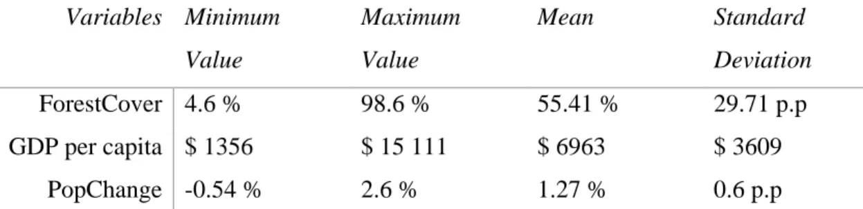
Table 2 describes the variables used together with its minimum, maximum, average

values as well as standard deviations.

Table 2 - Descriptive Statistics

Variables Minimum Value Maximum Value Mean Standard Deviation ForestCover 4.6 % 98.6 % 55.41 % 29.71 p.p GDP per capita $ 1356 $ 15 111 $ 6963 $ 3609 PopChange -0.54 % 2.6 % 1.27 % 0.6 p.p

Note: P.P presented in Table 3 is percentage points

The average GDP per capita for the continent of South America is USD 6963 from 1991-2019 and the average forest cover are 55.41 percent. Lowest forest cover is captured in Uruguay in 1991 and highest in Suriname 1991. Highest GDP per capita in South America is found in Chile 2018 and its opposite in Guyana 1999. The change in population reached its peak between the years 1990-91 in Paraguay and were decreasing in Guyana 1999. For full disclosure of each country, see Appendix.

Table 3 - Covariance Matrix

The correlation matrix in Table 3 shows a clear correlation between Urbanization and GDP per capita. This might affect the model and therefore the variable Urbanization is

ForestCover GDP per capita (GDP per capita)2 PopChange Urbanization ForestCover 1.000 -0.434 -0.437 0.050 -0.628 GDP per capita -0.434 1.000 0.973 -0.193 0.649 (GDP per capita)2 _{-0.437 0.973 1.000 -0.243 0.689} PopChange 0.050 -0.193 -0.243 1.000 0.059 Urbanization -0.628 0.649 0.689 0.059 1.000

20

not added to the regression, thus we do not conduct tests on model (3) and (5) since they contain the variable Urbanization.

4.2 Results

This study start the estimations of the results by examine the model for auto regressive errors and serial correlation the Wooldridge Approach for AR(1) is conducted. The null hypothesis is that no serial correlation between the variables exists and the alternative have the opposite. Model 4 in this study have insignificant coefficients and thus the Wooldridge Approach is conducted. In our case, we can reject the null hypothesis and thus conclude that there is evidence for serial correlation between the variables (see Appendix). Once serial correlation has been detected we adjust model 4 by using White period as robustness against large standard errors. The results can be seen in Table 4 for Model 4 adjusted.

The FEM results are presented in Table 4, showing the coefficients for all models and the standard errors.

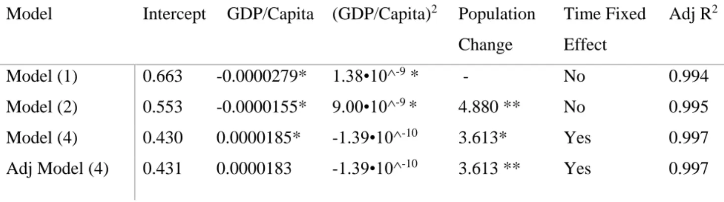
Both in Model (1) and (2) we find evidence of an EKCD since the coefficient for GDP per

capita (β1) is negative and the coefficient for (GDP per capita)2 is positive. In Model (1),

the coefficient for GDP per capita is negative, an increase in GDP per capita by USD 1 is suggested to decrease forest cover by 0.0000279 percent. On the contrary, (GDP per capita)2 _{is positive and an increase of USD 1 is suggested to increase forest cover by}

1.38*10-9 _{percent. Culas (2007) as well as Bhattari and Hammig (2001) obtain the same}

coefficient signs, meaning that when GDP per capita is negative, (GDP per capita)2 _is

positive and vice versa in their studies hence results and conclude that they have found an existence of an EKCD.

In the adjusted Model (4), an increase of USD 1 in GDP per capita will result in an increase in 0.0000183 percent in forest cover, simultaneously according to the model a 1

21

USD change in (GDP per capita)2 will reduce forest cover with 1.39*10-10 percent. These results are however not significant at a 5 percent or even 10 percent significant level.

We also find that the coefficient for population change (β3) is positive throughout our

models, a growth in population of one percent will result in an increase in forest cover by 3.61 percent. This result that a growth in population can have a positive impact on forest cover seems counter intuitive but can be due to a numerous reason such as technological improvement within the agricultural sector that have occurred during the period where population have increased in all countries with very few exceptions.

Adjusted R2 _{is high throughout all the models, and this points towards that the}

independent variables are describing the change in the dependent variable well and this can also be strengthened by results seen in previous research such as Ceddia (2013).

Table 4 - The relationship between Forest cover and GPD per capita

Model Intercept GDP/Capita (GDP/Capita)2 Population Change Time Fixed Effect Adj R2 Model (1) 0.663 -0.0000279* 1.38•10^-9 * - No 0.994 Model (2) 0.553 -0.0000155* 9.00•10^-9 * 4.880 ** No 0.995 Model (4) 0.430 0.0000185* -1.39•10^-10 3.613* Yes 0.997 Adj Model (4) 0.431 0.0000183 -1.39•10^-10 3.613 ** Yes 0.997

Note: 319 observations, from 11 countries (Venezuela have been dropped due to lack of

data) in South America 1991-2019.

* Denotes significance at 5%. ** Denotes significance at 10%.

4.3 Turning Point

Our EKCD is U-shaped in contrast to most of the previous research since we use share of

land covered by forest in contrast to the rate of deforestation. The turning point is calculated for models (1)-(2) and not for model (4) or adj model (4) since the coefficients are not significant either at a 5 percent confidence or 10 percent confidence and thus

22

calculate a turning point in those models would only contribute with faulty uncertain values. Model 1: − −2.79 • 10 −5 2 • 1.38 • 10−9 = 10 108.7 $ Model 2: − −1.55 • 10 −5 2 • 9.00 • 10−10 = 8 611.1 $

The turning point for Model 1 and 2 can be seen as realistic, the GDP per capita is higher than for all countries in South America, where the average GDP per capita for 2019 was USD 8364. However, the two countries that have experienced afforestation, Chile and Uruguay, had the highest GDP per capita of the 11 countries we conducted the study on with USD 15 091 and USD 14 957 respectively.

23

4.4 Robustness Checks

In order to make sure our models are robust and can be trusted it is of high importance to conduct robustness checks.

The long-run relationship is tested through a Johansen Fisher panel cointegration test. The result show cointegration between more than three variables of our regression, this is considered a possibility for us to regress every one of our variables without being spurious. The null hypothesis is rejected at every level of significance for which the results from the Johansen Fisher panel cointegration test can be found in the Appendix.

All variables are cointegrated in the long-run, therefore, one can move on to check between what kind of model to choose. The results from these tests can also be found in the Appendix. According to the Lagrange Multiplier test the REM is preferred to Pooled OLS at every significance level. A Hausman test is conducted, and the null hypothesis is not rejected meaning that a REM is preferred over FEM. Although a REM is preferred according to the Hausman test we follow the previous literature consistently using the FEM (e.g., Cropper & Griffiths, 1994; He et al., 2015) Further, in the theory of econometrics, it is suggested that parameters from the FEM are the most appropriate to apply in an analysis using cross-country samples as the FEM account for the structural and historical differences across countries (Greene, 1997).

24

5. Discussion

Our results confirm the existence of a U-shape EKCD with turning points of USD 10 108

and USD 8611 respectively, depending on the models used. The turning points calculated in this study is close to the current situation in some of the more developed countries in South America. The two countries that have experienced reforestation (Chile & Uruguay) during this time period have a higher GDP per capita at USD 15 091 and USD 14 957 respectively.

The results suggest that the patterns of increase in economic growth is considered to be a predominant cause of change in forest cover in South America. This is in line with what previous literature has found, Bhattarai and Hammig (2001) found existence of an EKCD

and a turning point for Latin America, to USD 6600 in 1985 nominal value. Transfer this into 2010 USD nominal value as used in this study, it equals USD 14 538. Barbier and Burgess (2010) claim to find evidence of an existing EKCD and calculate a turning point

of USD 4946. However, in their study they do not specify what year they use as a base year for the value of USD making it more difficult to compare. Additionally, they also suggest that GDP per capita and population growth is a profound cause of tropical deforestation.

During our study we see a positive effect on forest cover when population is increasing. In the paper written by Koop and Tole (1999) they find the EKCD to be USD 8660 for

Latin America and conclude that it is much higher than any Latin Americas current GDP per capita during that time. With regard to this, they also find evidence that population density tends to be positively associated with deforestation as well as population growth seems to have a mixed effect on forest cover. The mixed effect on forest cover by growth in population can be linked to the relationship between the Malthusian theory and Boserup theory. The Malthusian theory argues that, ceteris paribus, an increase in population will lead to an increased need for agricultural land, thus cutting down forest to provide more areas for food production. The Boserup theory, however, argues that technological improvements will occur and the output from existing agricultural practices will increase with improved technology. Agricultural expansion is one of the main drivers of deforestation and when population increases agricultural output will have to increase to

25

suffice. In the light of this, the results of our study points towards that the technological improvements within the agricultural sector have had more rapid improvements than the population increase and thus we see a positive relationship between population growth and forest cover.

As argued by Rudel and colleagues (2004), governmental policies regarding forests are more likely to occur in developing countries where there are scarce levels of forest. This can be one of the reasons that we have seen Chile and Uruguay having afforestation during the period for this study since they have less share of land covered by forest in comparison with for instance, Brazil. This point towards that it is more effective to control deforestation and improve the environment by implementing aggressive environmental policies rather than limiting economic and population growth. Panayotou (1997) proclaimed that such policies are likely to have lower costs and be more beneficiary than to try to force restrictions on economic and population growth.

The conservation of existing forest and increased productivity in agriculture land is key to maintain world’s biodiversity and secureness of, for instance, food within rural areas which has a direct connection to expansion in agricultural land with increase soy production and cattle ranching (FAO & UNEP, 2020). One reason to why it is important to study the relationship between forest cover and economic development is to obtain evidence for the need of strong institutions, better regulations and extensive environmental policies. This requires a government that is effective and has a mutual respect for the knowledge and rights of local rural communities as well as their biodiversity. Economic development is not the single variable that is of importance, however, higher economic development seems to have a strong positive effect on government performance and that richer countries are less interventionist meaning they protect property rights better and regulate better (Porta et al., 1999).

This study is restricted to the continent of South America, however there is large differences between the countries within the sample. Furthermore, Uruguay has a forest cover of roughly 10 percent and a GDP per capita USD 14 957 for 2019 comparing to Guyana that have a forest cover above 90 percent and GDP per capita roughly USD 6000. This can lead to a model that will be a bit skewed as there are statistical outliners within

26

the sample. The FEM, however, controls for some of the difference between the countries such as difference in culture, geography and history. Political ruling is not controlled for in FEM as this potentially can change several times during the time period of this study. We however controlled for this and other year fixed effects by including year dummy variables in our model. There are some questions in regards of the data used in this study. For instance, we are using data for forest cover on national levels collected from the Food and Agriculture Organization of the United Nations (FAO), in 11 different countries in South America. The data is the most complete data found on forest cover in South America, but the data is not 100 percent accurate, and one should acknowledge the possibility of flaws in the dataset regarding forest cover. The GDP per capita is also on a national level but is more reliable and the same can be said about the data on population. The time frame used is from 1991-2019 and thus 28 years since we could not find complete data before 1991.

There is a possibility that a more advanced model with more independent variables such as debt of a country, sociological factors, import, export, infrastructure and government interference and trust in governments can change the result and give a more wholesome picture of how the share of land covered by forest is affected. Data for this is however not easy to find and/or validate for the period of 1991-2019. Variables such as infrastructure are a cause for loss in forest cover, however, may be closely correlated with income (Stern, 2004). Variables related to agricultural land expansions are a cause to loss in forest cover however there is a close negative correlation between forest cover and agricultural land (Benhin, 2006).

27

6. Conclusion

The relationship between change in forest cover and economic development, the so-called Environmental Kuznets Curve for deforestation (EKCD) has been highly studied (e.g.

Barbier & Burgess 2001, Bhattarai & Hammig 2001, Culas 2007). However, the results are still ambiguous. In this paper we test the hypothesis of that change in forest cover in South America is U-shaped EKCD. We use panel data from 1991 to 2019 on forest cover

and GPD per capita for all South American countries (except Venezuela due to lack of data) and provide evidence for a U-shaped EKCD. We find the turning points of the EKC

to be between USD 10 108 and USD 8611. Also, we noticed that both GDP per capita and population change have a significant impact on change in forest cover when it comes to South America. Our study contributes to the academic field by providing evidence for the existence of an EKCD for forest cover in South America. This is in line with what

previous studies also did found evidence for existence of an EKCD although, both Bhattari

and Hammig (2001) as well as Barbier and Burgess (2001) conducted their studies on Latin America, with turning points of USD 6600 and USD 4946, respectively. With the former based in 1985 nominal value and transferred into 2010 USD nominal value as used in this study, it equals USD 14 538 and the latter do not specify which base year. They also suggest that GDP per capita and population change is a predominant cause of deforestation, which strengthens our result with GDP per capita having a negative effect on change in forest cover and population growth the opposite.

This is perhaps the most updated dataset and unique in its solely focus on South America. However, as in all academia research, our study faced limitations. We wanted to conduct research containing factors of socio-institutional policies but as the dataset within this is hard to collect, we could not fulfil. Additionally, one could investigate how determination of forest management is affecting livelihoods and its connection to profits as well as the problem of conducting data on adequate policies and institutions. However, it is an important to acknowledge the importance of government policies when it comes to change in forest cover. Further researchers should consider conducting paper on regional levels and with data on environmental policies adding trust in government and corruption as variables rather than more indicators of economic development. To shed light on a

28

more regional micro level research is needed to investigate the true relationship of how people and communities are affected by the change in forest cover.

29

Reference list

Angelsen, A. M. Brockhaus, M. Kanninen, E. Sills, & W. D. Sunderlin (Eds.), (2009). Realising REDD+: National strategy and policy options (p. 4), Bogor, Indonesia: Center for International Forestry Research (CIFOR).

Achard, F., Eva, H.D., Stibig, H.J., Mayaux, P., Gallego, J., Richards, T., Malingreau, J-P. (2002) Determination of Deforestation Rates of the World’s Humid Tropical Forests.

Science Vol 297 Page 999-1002. Retrieved from:

https://www.researchgate.net/profile/Philippe-Mayaux/publication/11216758_Determination_of_Deforestation_Rates_of_the_World %27s_Humid_Tropical_Forests/links/0912f50cb0057798af000000/Determination-of-Deforestation-Rates-of-the-Worlds-Humid-Tropical-Forests.pdf

Atmadja, S., Sills, E. (2015). Identifying the causes of Tropical deforestation: Meta-analysis to test and develop economic theory. Tropical Forestry Handbook, 1-27. doi:10.1007/978-3-642-41554-8_252-1

Azomahou T, Laisney, F. Van, P.N Economic development and CO2 emissions: A nonparametric panel approach. Journal of Public Economics 90 (2006)

Bae, J.S., Joo, R.W., Kim, Y.S., (2012) Forest Transition in South Korea: Reality, Path and Drivers. Land Use Policy Volume 29 Page 198-207.

doi.org/10.1016/j.landusepol.2011.06.007

Barbier E.B, Burgess J.C (2001) The economics of tropical deforestation. Journal of

economic surveys vol 15 no 3. Page 413-433 Doi:10.1111/1467-6419.00144

Benhin, J. K. A. (2006). Agriculture and deforestation in the tropics: A critical theoretical and empirical review. Ambio, 35(1), 9-16. Retrieved from

http://proxy.library.ju.se/login?url=https://www.proquest.com/scholarly- journals/agriculture-deforestation-tropics-critical/docview/207673092/se-2?accountid=11754

Bhattacharyya, S, Hodler, R, (2009) Natural Resources, democracy and corruption. European Economic Review 54 page 608-621 doi:10.1016/j.euroecorev.2009.10.004 Bhattarai, M, Hammig, M (2001) Institutions and the Environmental Kuznets Curve for Deforestation: A Crosscountry Analysis for Latin America, Africa and Asia. World

30

Boserup, E. (1970). The conditions of agricultural growth: The economics of agrarian change under population pressure. London: Allen and Unwin. Retrieved from:

https://www.biw.kuleuven.be/aee/clo/idessa_files/boserup1965.pdf

Breusch T.S & Pagan A.R (1980) Econometrics Issue. The Review of Economic Studies, Vol. 47, No. 1, pp. 239-253 Retrieved from: https://www.jstor.org/stable/2297111 Burgess, R., Hansen, M., Olken, B., Potapov, P., Sieber, S. (2011). The Political Economy of Deforestation in the Tropics. https://doi.org/10.3386/w17417

Ceddia, M. G., Bardsley, N. O., Gomez-y-Paloma, S., & Sedlacek, S. (2014). Governance, agricultural intensification, and LAND sparing in tropical South America. Proceedings of the National Academy of Sciences, 111(20), 7242-7247.

doi:10.1073/pnas.1317967111

Choumert, J., Combes Motel, P., & Dakpo, H. K. (2013). Is the ENVIRONMENTAL Kuznets curve for deforestation a Threatened theory? A meta-analysis of the literature.

Ecological Economics, 90, 19-28. doi:10.1016/j.ecolecon.2013.02.016

Chowdhury, R., & Moran, E. F. (2012). Turning the curve: A critical review of kuznets approaches. Applied Geography, 32(1), 3-11

https://doi.org/10.1016/j.apgeog.2010.07.004

Cochrane, D.; Orcutt, G. H. (1949). "Application of Least Squares Regression to Relationships Containing Auto-Correlated Error Terms". Journal of the American Statistical Association. 44 (245): 32–61. doi:10.1080/01621459.1949.10483290. Cole, M.A., Rayner, A.J., Bates, J.M., 1997, The Environmental Kuznets curve: An empirical analysis. Environmental and Development Economics Volume 2 page 401-416. doi:10.1017/S1355770X97000211

Cropper, M., & Griffiths, C. (1994). The Interaction of Population Growth and Environmental Quality. The American Economic Review, 84(2), 250-254. Retrieved from http://www.jstor.org/stable/2117838

Claudine Egger, Helmut Haberl , Karl-Heinz Erb & Veronika Gaube (2020) Socio-ecological trajectories in a rural Austrian region from 1961 to 2011: comparing the theories of Malthus and Boserup via systemic-dynamic modelling, Journal of Land Use Science, 15:5, 652-672, doi: 10.1080/1747423X.2020.1820593

Culas, R.J (2007) Deforestation and the Environmental Kuznets Curve: An institutional Perspective. Ecological Economics 61 Page 529-437

31

Dinda, S Environmental Kuznets Curve Hypothesis: A survey. Ecological Economics 49 (2004) doi.org/10.1016/j.ecolecon.2004.02.011

FAO and UNEP. 2020. The State of the World’s Forests 2020. Forests, biodiversity and people. Rome. doi.org/10.4060/ca8642en

Grau, H.R, Gasparri, N.I, Mitchell Aide T. (2005) Agriculture expansion and deforestation in seasonally dry forests of north-west Argentina. Foundation for

Environmental Conservation 32(2) 140-148. doi:10.1017/S0376892905002092

Hansen, M.C., Potapov, PV., Moore, R., Hancher, M., Turubanova, S.A., Tyukavina, A., Thau, D., Stehman, S.V., Goetz, S.J., Loveland, T.R., Kommareddy, A., Egorov, A., Chini, L., Justice., C.O., Townshend, J.R.G. (2013) High-Resolution Global Maps of 21st_{-Century Forest Cover Change. Science Volume 342 Page 850-852 retreived from:}

https://storage.googleapis.com/pub-tools-public-publication-data/pdf/42119.pdf Hausman J. A Econometrica , Nov., 1978, Vol. 46, No. 6 (Nov., 1978), pp. 1251-1271 retrieved from: http://www.jstor.org/stable/1913827

He, Z, Xu, S , Shen, W, Long, R, Chen, H. Impact of urbanization on energy related CO2 emission at different development levels: Regional difference in China based on panel estimation. Journal of Cleaner Production 140 (2017).

https://doi.org/10.1016/j.jclepro.2016.08.155

Hosonuma, N., Herold, M., De Sy, V., De Fries, R., Brockhaus, M., Verchot, L., Angelsen, A., & Romijn, E. (2012). An assessment of deforestation and forest degradation drivers in developing countries. Environmental Research Letters, 7(4), 44009–. https://doi.org/10.4060/ca8642en

Koop, G & Tole, L (1999) Is there an environmental Kuznets curve for deforestation?

Journal of Development Economics Vol. 58 Page 231-244.

https://doi.org/10.1016/S0304-3878(98)00110-2

Lim, A.S.K & Tang, K.K., (2008) Human Capital Inequality and the Kuznets Curve.

The Developing Economies. Volume 46(1) page 26-51. doi:

10.1111/j.1746-1049.2007.00054.x

Maddala, G. S. and S. Wu (1999). “A Comparative Study of Unit Root Tests with Panel Data and A New Simple Test, “Oxford Bulletin of Economics and Statistics, 61, 631-52. Retrieved from: https://onlinelibrary.wiley.com/doi/pdf/10.1111/1468-0084.0610s1631 Malthus, T. (1798). An essay on the principle of population.

32

Mather, A. (1999). The forest transition: Passage to sustainability. Brookfield, VT: Ashgate Pub.

Mahapatra, K., & Kant, S. (2005). Tropical deforestation: A multinomial logistic model and some country-specific policy prescriptions. Forest Policy and Economics, 7(1), 1-24. https://doi.org/10.1016/S1389-9341(03)00064-9

Mena, C.F, Bilsborrow R.E, McClain, M.E. Socioeconomic Drivers of Deforestation in the Northern Ecuadorian Amazon. Environmental Management Vol. 37(6) page 802-815. doi: 10.1007/s00267-003-0230-z

Cole, M.A. Rayner A.J and Bates J.M (1997) The environmental Kuznets curve: an empirical analysis. Environment and Development Economics, 2, pp 401416 doi:10.1017/S1355770X97000211

Moomaw and Shatter 1996, Urbanization and Economic Development: A Bias Towards Large Cities. Journal of Urban Economics 40, 1996 Page 13-37

https://doi.org/10.1006/juec.1996.0021

Müller, H., Griffiths, P., Hostert, P., (2016) Long-Term deforestation dynamics in the Brazilian Amazon-Uncovering historic frontier development along the Cuiabá-Santarém highway. International Journal of Applied Earth Observation and Geoinformation Volume 44 page 61-69. https://doi.org/10.1016/j.jag.2015.07.005

Ometto, J.P, Dutra Aguilar A.P, Martinelli, L.A. (2011) Amazon deforestation in Brazil: effects, drivers and challenges. Carbon Management 2:5 575-585.

doi:10.4155/cmt.11.48

Panayotou, T (1997) Demystifying the Environmental Kuznets Curve: Turning a black box into a Policy tool. Environmental and Development Economics Volume 2 Page 465-484. doi:10.1017/S1355770X97000259

Perz, S.G., (2007) Grand Theory and Context-Specificity in the Study of Forest Dynamics: Forest Transition Theory and Other Directions, The Professional Geographer, 59:1, 105-114, doi: 10.1111/j.1467-9272.2007.00594.x

Porta, Lopez-de-Silanes, Shleifer & Vishny,1999 Investor protection and corporate

governance Journal of Law, Economics & Organization Volume 15 no 1. Pp 222-279

https://doi.org/10.1016/S0304-405X(00)00065-9

Renoir, M. R & Guttentag, M. G. (2018). Facilitating financial sustainability: Understanding the drivers of Deforestation and financial sustainability. doi:10.15868/socialsector.30588

33

Rudel, T. K., Coomes, O. T., Moran, E., Achard, F., Angelsen, A., Xu, J., & Lambin, E. (2005). Forest transitions: Towards a global understanding of land use change. Global

Environmental Change, 15(1), 23-31. doi:10.1016/j.gloenvcha.2004.11.001

Scrieciu, S. S. (2007). Can economic causes of tropical deforestation be identified at a global level? Ecological Economics, 62(3-4), 603-612.

doi:10.1016/j.ecolecon.2006.07.028

Stern, D 2018. Reference Module in Earth Systems and Environmental Sciences Journal Amsterdam. Retrieved from

https://reader.elsevier.com/reader/sd/pii/S0304387898001102?token=F39FE89CF67015 AD097E331C4EDAEFCFE919C108DBF0F8897E04AFD46B67F1561C8EEB2A2C95 49B6D42CDBFFABF1DAD6

Song, X-P, Huang, C, Saatchi, SS , Hansen, MC, Townshend, JR. (2015) Annual Carbon Emissions from Deforestation in the Amazon Basin between 2000 and 2010. PLoS ONE 10(5) doi:10.1371/journal.pone.0126754

Transparency International. (2011), Global corruption report: Climate change. (2011). Retrieved from:

https://images.transparencycdn.org/images/2011_GCRclimatechange_EN.pdf

Velasco Gomez, M.D., Beuchle, R., Shimabukuro, Y., Grecchi, R., Simonetti, D., Eva, H.D., Achard, F., (2015) A Long-Term Perspective on Deforestation Rates in the Brazilian Amazon. The International Archives of the Photogrammetry, Remote Sensing

and Spatial Information Science, Volume XL-7/W3 Page 539-544.

doi:10.5194/isprsarchives-XL-7-W3-539-2015

Vuong, QH., Ho, MT., Nguyen, HK.T. et al. The trilemma of sustainable industrial growth: evidence from a piloting OECD’s Green city. Palgrave Commun 5, 156 (2019). https://doi.org/10.1057/s41599-019-0369-8

Van Nguyen, P, Azomahou, T., (2007) Nonlinearities and heterogeneity in

environmental quality: An empirical analysis of deforestation. Journal of Development

Economics 84 Page 291-309 doi:10.1016/j.jdeveco.2005.10.004

Yeo, I.Y., Huang, C., (2012) Revisiting the forest transition theory with historical records and geospatial data: A case study from Mississippi (USA) Land Use Policy

34

Appendix

Appendix 1 – Descriptive Statistics

List of countries and change over period of time.

ARGENTINA Forestcover GDP/capita Popchange Urbanization level

1991 12.80% $6 721 - 87.33%

2004 11.70% $7 962 14.06% 89.86%

2019 10.50% $9 742 26.39% 91.99%

BOLIVIA ForestCover GDP/capita PopChange Urbanization Level

1991 53.10% $1 398 - 56.58%

2004 50.10% $1 657 22.69% 63.71%

2019 47.10% $2 579 39.10% 69.77%

BRAZIL ForestCover GDP/capita PopChange Urbanization Level

1991 70% $7 963 - 74.69%

2004 64% $9 346 21.86% 82.52%

2019 60% $11 121 28.40% 86.82%

CHILE ForestCover GDP/capita PopChange Urbanization Level

1991 20.60% $6 291 - 83.40%

2004 21.80% $10 726 15.73% 86.72%

2019 24.30% $15 091 28.79% 87.64%

COLOMBIA ForestCover GDP/capita PopChange Urbanization Level

1991 58.30% $4 468 - 83.40%

2004 55.80% $5 225 19.77% 75.62%

2019 53.50% $7 838 32.94% 87.64%

ECUADOR ForestCover GDP/capita PopChange Urbanization Level

1991 58.60% $3 786 - 55.71%

2004 54.20% $4 112 22.98% 61.51%

2019 50.60% $5 097 39.72% 63.99%

GUYANA ForestCover GDP/capita PopChange Urbanization Level

1991 94.50% $2 394 - 29.49%

2004 94.20% $3 794 0.17% 28.06%

2019 93.60% $6 107 5.04% 26.69%

35

1991 63.70% $3 577 - 49.44%

2004 54.40% $3 569 24.36% 57.30%

2019 41.20% $5 310 38.47% 61.88%

PERU ForestCover GDP/capita PopChange Urbanization Level

1991 98.60% $2 654 - 69.30%

2004 98.20% $3 604 18.47% 74.64%

2019 97.50% $6 486 30.72% 78.10%

SURINAME ForestCover GDP/capita PopChange Urbanization Level

1991 98.60% $6 131 - 65.78%

2004 98.20% $6 971 16.34% 66.68%

2019 97.50% $8 046 28.96% 66.10%

URUGUAY ForestCover GDP/capita PopChange Urbanization Level

1991 4.90% $7 071 - 89.30%

2004 8.60% $8 449 5.72% 93.08%

2019 11.50% $14 597 9.54% 95.43%

VENEZUELA ForestCover GDP/capita PopChange Urbanization Level

1991 58.70% $12 830 - 84.66%

1998 55.70% $11 944 17.30% 87.56%

2014 53.10% $14 025 29.53% 88.14%

Note: The percentage change in population is calculated from the year of 1991 for both

2004 and 2019 for all countries except for Venezuela where the change in population is calculated from 1991 for 1998 and 2014 respectively. Hence are dropped from the regression model.