Phase-field modeling of stress-induced precipitation and kinetics in engineering metals

(1)

THESIS FOR THE DEGREE OF DOCTOR OF PHILOSOPHY

Phase-field modeling of stress-induced precipitation and

kinetics in engineering metals

CLAUDIO F. NIGRO

Department of Industrial and Materials Science

CHALMERS UNIVERSITY OF TECHNOLOGY Gothenburg, Sweden 2020

(2)

i

Phase-field modeling of stress-induced precipitation and kinetics in engineering materials  CLAUDIO F. NIGRO 

Gothenburg, Sweden, 2020 ISBN: 978-91-7905-337-6

Doctoral thesis at Chalmers University of Technology Series number 4804  

ISSN 0346-718X

Department of Industrial and Materials Science Chalmers University of Technology

SE-412 96 Gothenburg Sweden Telephone + 46 (0)31-772 1000 Printed by Chalmers Reproservice Gothenburg, Sweden 2020

(3)

ii

Phase-field modeling of stress-induced precipitation and kinetics in engineering metals CLAUDIO NIGRO

Department of Industrial and Materials Science CHALMERS UNIVERSITY OF TECHNOLOGY

Abstract

The formation of brittle compounds in metals operating in corrosive environments can be a tremendous source of embrittlement for industrial structures and such phenomenon is commonly enhanced in presence of stresses. To study this type of microstructural change modeling is preferred to experiment to reduce costs and prevent undesirable environmental impacts. This thesis aims at developing an engineering approach to model stress-induced precipitation, especially near stress concentrators, e.g. crack tips, for multi-phase and polycrystalline metals, with numerical efficiency.

In this thesis, four phase-field models are developed and applied on stress-induced hydride precipitation in zirconium and titanium alloys. The energy of the system is minimized through the time-dependent Ginzburg-Landau equation, which provides insights to the kinetics of the phenomenon. In these models, the driving force for precipitation is the coupling between the applied stress and the phase transformation-induced dilatation of the system. Models 1-3 implicitly incorporate near crack-tip stress fields by using linear elastic fracture mechanics so that only the phase-field equation is solved numerically with the finite volume method, reducing the computational costs. Phase transformation is investigated for intragranular, intergranular and interphase cracks in single- and two-phase materials by considering isotropy and some degrees of anisotropy, grain/phase boundary energy, different transition orders and solid solubility limit. Model 4 allows representing anisotropy connected to lattice mismatch and the orientation of the precipitates influenced by the applied stress. The model is employed through the finite element program Abaqus, where the fully coupled thermo-mechanical solving method is applied to the coupled mechanical/phase-field problem. Hydride growth is observed to follow the near-crack tip hydrostatic stress contours and can reach a steady state for specific conditions. The relation between hydride formation kinetics and material properties, and stress relaxation are well-reflected in the results.

With the presented approaches, precipitation kinetics including different kinds of defects, multi-phase microstructures, phase/grain boundaries, order transitions and loading modes can be successfully captured with low computational costs. They could therefore contribute to the numerical efficiency of multi-scale environment-assisted embrittlement prediction schemes within commercial software serving engineering projects.

Keywords: phase transformation, phase-field theory, corrosion, hydrogen embrittlement, hydride, linear elastic fracture mechanics, finite volume method, finite element method

(4)

(5)

iv

(6)

(7)

vi

To know that we know what we know, and to know that we do not know what we

do not know, that is true knowledge.

(8)

vii

Faculty of Technology and Society

Department of Materials Science and Applied Mathematics MALMÖ UNIVERSITY

(9)

viii

Acknowledgements

This PhD work has taken place in the department of Material Science and Applied Mathematics at the Faculty of Technology and Society, Malmö University in cooperation with the department of Industrial and Materials Science at Chalmers University of Technology. This work was funded by Malmö University.

I would like to thank my supervisors, Christina Bjerkén, Ylva Mellbin and Pär Olsson, for supporting me throughout this project by providing their expertise, knowledge and encouragements. I am also grateful to the whole team within material science and mechanics at Malmö University for welcoming and integrating me with kindness and professionalism. I wish to give a special acknowledgement to my former colleague and friend Niklas Ehrlin who shared numerous exciting PhD student activities and interesting discussions.

I wish to thank my collaborators in the project CHICAGO (Crack-induced HydrIde nuCleation And GrOwth), which is a collaboration between the teams of Lund University and Malmö Univeristy. The members, Wureguli Reheman, Martin Fisk, Christina Bjerkén, Per Ståhle, Pär Olsson and I, have allowed carrying out a common project and contributed to the writing of the appended Paper E.

Special and obvious thanks are addressed to my wife Pernilla and my two sons, Henri and Arthur, the brightest sunshines of my life, for their support and understanding. I am also grateful for the endless encouragements and additional support given by my parents, sister, brother, parents-in-law, cousins and closest friends.

Claudio Nigro Malmö, Sweden October 2020

(10)

(11)

x

List of publications

This thesis is based on the work contained in the following papers:

Paper A

Claudio F. Nigro, Christina Bjerkén, Pär A. T. Olsson. Phase structural ordering kinetics of second-phase formation in the vicinity of a crack, 209, 91–107. Published in the International

Journal of Fracture, 2018.

Paper B

Claudio F. Nigro, Christina Bjerkén, Pär A. T. Olsson. Kinetics of crack-induced hydride formation in hexagonal close-packed materials. Published in the Proceedings of the 2016

International Hydrogen Conference, 2016.

Paper C

Claudio F. Nigro, Christina Bjerkén, Ylva Mellbin. Modelling of a Crack-Induced Hydride Formation at a Grain Boundary in Metals. Accepted for publication in the International

Journal of Offshore and Polar Engineering, 2020.

This paper is an extension of:

Claudio F. Nigro, Christina Bjerkén, Ylva Mellbin, Modelling of a Crack-Induced Hydride Formation near a Grain Boundary in Metals, Published in the Proceedings of the 29th

International Ocean and Polar Engineering Conference, 2019

Paper D

Claudio F. Nigro, Christina Bjerkén, Ylva Mellbin. Phase-field modelling: effect of an interface crack on precipitation kinetics in a multi-phase microstructure. Submitted to the

International Journal of Fracture, 2020

Paper E

Wureguli Reheman, Claudio F. Nigro, Martin Fisk and Christina Bjerkén. Kinetics of Strain-Induced Precipitation - Phase-Field Model and Fully Coupled FE Approach. Manuscript form.

Own contribution

In Paper A, B, C and D, the author of this thesis carried out all simulations, numerical implementations and analyzed the results. He planned the entire work for Paper B, C and D. The co-authors participated in writing the manuscripts and planning the work for Paper A and contributed to the elaboration of all papers through discussions. For Paper E, the author of this thesis took an active part in the planning of the work, and worked on the numerical implementation, the development of the model and the manuscript writing.

(12)

(13)

xii

1 Introduction

Hydrogen, the most abundant and lightest chemical element in the universe, has become a major concern for the material industry. Numerous works have shown that it is responsible for degrading the mechanical properties of metals in hydrogen-rich environments, possibly leading to premature fracture [1].

Hydrogen embrittlement (HE) is generally characterized by the deterioration of the mechanical properties of a material in presence of hydrogen. The phenomenon is well-known in aerospace and nuclear industries. In rocket engines, developed for Ariane 6 such as Vinci and Vulcain 2, hydrogen is thought to be utilized as fuel and cooler and, therefore, interacts with some engine components. The mechanical properties of nickel-based superalloys, traditionally used in high-temperature areas such as the combustion chamber [2] and the nozzle, have been observed to be derogated in presence of hydrogen [3, 4]. Brittle compounds, titanium hydrides, are likely to form in colder engine parts made of titanium alloys when in contact with hydrogen and can embrittle the structure. In nuclear reactor pressure vessels, atomic hydrogen (H) penetrates zirconium-based cladding and pressure tubes, where brittle zirconium hydrides potentially form [5, 6]. Hydride formation is one stage of the complex mechanism of delayed hydride cracking (DHC) [7, 8], which is one of the most notorious mechanisms of HE in nuclear industry. Hydride precipitation, strongly influenced by the presence of stress [9], can be enhanced by the presence of material defects acting as stress concentrators [10]. Knowledge of hydride formation kinetics is fundamental in order to predict the lifetime of a metallic structure subjected to hydride-based failure processes, such as DHC in a hydrogen-rich environment. Modeling is found to be an economically beneficial route to study the growth of hydride phase regions in a metallic structure operating in a hydrogen-rich environment and under applied load. Second-phase formation has been modeled over the years through the use of different approaches such as the sharp-interface and phase-field methods (PFM). The latter is found to be more practical to model complex microstructures with numerical efficiency and can include stress effect on precipitation [11, 12, 13].

This thesis is included in a project, which aims at building an engineering tool to model stress-induced precipitation and kinetics, and to design the product to be numerical efficient and easily implementable in commercial software. Within this framework, the objective of the work is to develop a numerical approach for modeling of precipitation, especially in the vicinity of stress concentrators, such as crack tips, and at grain and phase boundaries.

In the present thesis, different approaches based on phase-field theory (PFT) are developed. Linear elastic fracture mechanics (LEFM) is adopted in three of the four presented models in order to account for the stress field near an opening sharp crack. With these models, many aspects such as the solid solubility limit, the transition temperature, the interfacial energy, the applied stress, the energy of phase and grain boundaries, the transition order and some forms of anisotropy are incorporated in the considered problems, which are solved by using the finite volume method (FVM). These approaches are also flexible in terms of applications and formulated optimally such that the considered microstructural evolutions are captured with

(18)

2

numerical efficiency. The latter is partly due to the fact that only the equation related to phase transformation needs to be solved numerically while mechanical equilibrium is calculated analytically. The fourth approach is still a pilot model and is written to account for stress-induced second-phase formation, where the anisotropic dilatation of the material caused by phase transformation in relation with the orientation of the second-phase regions is addressed. With this model, the applied stress and defects are represented explicitly by choosing appropriate meshes and boundary conditions. The coupled mechanical and phase field-related equations are solved simultaneously by using the finite element method (FEM) associated to a fully coupled approach similar to that employed to solve thermo-mechanical problems. The application of the numerical methodology to the presented problems has been made possible thanks to the capacities and customizable subroutines of the commercial software Abaqus [14].

In this work, all mathematical approaches are applied to model stress-induced hydride formation. Crack-induced hydride formation is regarded with models 1-3 while hydride precipitation in a hydrogenated defect-free medium and near a notch tip is considered with model 4. Nevertheless, all presented models could also be employed to study environment-assisted degradation mechanisms, other than HE, involving the precipitation of brittle phases in materials operating in corrosive environment, e.g. rust or carbide formation in steel.

In this PhD thesis, the physical aspects and mathematical tools as the basis of this work are presented before the different models introduced above are described. Thereafter, the results obtained in the papers are reported and thoughts about futures developments are discussed. Parts of this document are taken and/or rephrased from the author’s licentiate thesis [15].

(19)

3

2 Environment-assisted degradation

2.1 Introduction to corrosion in metals

In operation, most metallic structures are observed to interact with their environments. Such interactions can affect the appearance of the metals and their physical properties, e.g. their mechanical properties. Corrosion is one deteriorative process, which is characterized by a destructive, unintentional and electrochemical attack of metals usually starting at their surface. There are several forms of corrosion such as uniform attack, galvanic corrosion, crevice corrosion, pitting, erosion-corrosion, selective leaching, intergranular corrosion, stress corrosion and HE [16].

Through intergranular corrosion, some stainless-steel structures experience failure along their grain boundaries. In the latter region, chromium, usually added to increase corrosion resistance, reacts with carbon to form chromium carbide. The regions adjacent to the grain boundary result depleted of chromium and, consequently, become more vulnerable to corrosion. The grain and phase boundaries are usually preferential site for precipitation because the nucleation energy barrier is lower and diffusion is quicker therein [17].

Some materials, which usually do not experience any form of corrosion in corrosive environments, can display reaction of corrosion when subjected to tensile stress or residual stresses. Cracks can nucleate in these areas, propagate and possibly lead to structure failure. This form of corrosion is named stress corrosion and the phenomenon is commonly referred to as stress corrosion cracking. In steels, rust, a brittle phase with lower fracture toughness than the rest of the material, can appear in material regions where stress is located and, subsequently, fracture. For instance, iron oxide can be seen to precipitate in welds and pipe bends, where residual stresses reside. Stress corrosion cracking results in brittle fracture regardless of the degree of ductility of the affected metal and may occur for stresses significantly below the fracture toughness [16].

2.2 Hydrogen embrittlement

2.2.1 Forms of hydrogen damage

The presence hydrogen in metals, such as steels, aluminum (Al), titanium (Ti), zirconium (Zr), nickel (Ni) and their respective alloys, can alter the properties of the material. As for stress corrosion, failures can arise from residual and/or applied tensile stresses combined with hydrogen-metal interactions in hydrogen-rich environments. Such interactions are commonly found to cause loss of ductility and reduction of load-carrying capacity in a metal. The term hydrogen embrittlement is used to refer to such deteriorations of materials. Stress corrosion and HE are similar in that normally ductile materials undergo brittle fracture when subjected to stress and corrosive environment. One difference between the two phenomena is that stress corrosion usually occurs in material regions, where anodic reactions take place, while hydrogen environment embrittlement can be initiated or enhanced by cathodic reactions, e.g. in the presence of a cathodic protection. Hydrogen environment embrittlement characterizes situations where materials undergo plastic deformation, while in contact with hydrogen-rich

(20)

4

gases or corrosion reactions. Molecular hydrogen experiences adsorption at the metal free surface, which weakens the H-H bond and favors its dissociation into atomic hydrogen within the metal lattice [18, 19]. Several other types of hydrogen damage mechanisms are known as hydrogen attack, blistering, and hydride formation [1], hydrogen enhanced localized plasticity (HELP) and hydrogen-induced decohesion (HID). Hydrogen attack usually affects steels at high temperature. The inner hydrogen reacts with carbon to form methane within the material. Possible damaging consequences are crack formation and decarburization. Blistering is the result of plastic deformation induced by the pressure of molecular hydrogen that is formed near internal defects. The gas formation occurs due to the diffusion of atomic hydrogen to these regions. Once formed, blisters are often observed to be fractured. The HELP mechanism is characterized by an enhancement of the mobility of dislocations by interaction with hydrogen [20]. In other cases, the presence of hydrogen can induce a reduction in the bonding energy between atoms, which consequently increases the risk of decohesion [21]. This mechanism is the so-called HID.

2.2.2 Hydride formation in titanium- and zirconium-based metals

During service and in presence of hydrogen, the formation of brittle and non-metallic compounds, the so-called hydrides, can be responsible for material embrittlement [5, 7, 22]. A number of materials such as zirconium, titanium, hafnium, vanadium and niobium are considered as hydride forming metals as they have a low solubility of hydrogen, and, therefore, can form different types of hydride phases depending on e.g. hydrogen concentration and temperature history [8]. This section is focused on briefly describing hydridation and its effect on mechanical properties in Zr- and Ti-based metals.

Pure titanium and zirconium microstructures have two different possible crystal structures: α, a hexagonal close-packed (HCP) microstructure at low temperature, and β, a body-centered cubic (BCC) microstructure at elevated temperatures. For pure Ti and Zr, the transition between these phases occurs through an allotropic transformation at 882°C and 862°C respectively. The dissolution of alloying elements can be done to stabilize different phases by modifying the α-β transition temperature or to cause solid solution strengthening. While a number of interstitial elements such as nitrogen, carbon, and oxygen act as α-stabilizers, the addition of hydrogen to the solid solution induces the stabilization of the β-phase by lowering the transus temperature. This can also be seen when considering the Zr-H and the Ti-H phase diagrams in Figure 1. The solid solution phase  has a low solubility of hydrogen while the high-temperature allotrope -Zr has a high solid solubility limit. In fact, for Ti, phase α possesses a maximum solubility of hydrogen equal to 4.7 at.% and for phase β it is equal to 42.5 at.% at 298°C. This can be imputed to the affinity of hydrogen for tetrahedral interstitials, which are twelve in the BCC phase and four in the HCP one [23]. For a given concentration of hydrogen and range of temperature, the phase diagrams exhibit regions of existence and stability (or metastability) of hydride phases [24, 25]. For both metals, two stable hydride phases are identified to be the centered cubic (FCC) -phase and the face-centered tetragonal (FCT) -phase. The -phase is considered metastable and has an FCT structure [26, 27]. Additionally, for the Zr-H system, a crystal structure denoted  has been observed and may be a possible precursor to the formation of - and -phases [28]. The

(21)

Ti-5

hydride χ, which forms at 41-47 at.% hydrogen at temperatures around -200 °C is rarely observed [23].

(a) (b)

Figure 1: Phase diagram for (a) the Zr-H system, (reproduced and modified with permission from [29]), and (b) the Ti-H system (sketch based on [25]).

The hydride precipitates generally appear as needles or platelets in the -phase, and the formation can occur either in grains or grain/phase boundaries in polycrystals [5, 8, 30, 31]. A preferred hydride orientation may exist and is affected by the crystal structure and texture emanating from the manufacturing process and the possible presence of applied and residual stresses [7, 9]. Under a sufficiently high applied load, the hydride platelets usually form perpendicular to the applied stress [6].

Some hydrides such as - and -hydrides in Zr- and Ti-based alloys exhibit a volume change when they form [26, 27]. For instance, the global swelling of the unconstrained - and -r hydrides, which results from anisotropic dilatational misfits, has been theoretically estimated to be between 10% and 20% with respect to untransformed zirconium [32]. The deformations induced by phase transformation can also be referred to as eigenstrains, stress-free strains or phase-transformation strains. The hydrides are more brittle than the -phase, and the fracture toughness of a hydride can be orders of magnitude lower than the solid solution. For example, the fracture toughness 𝐾_𝐼𝐶 of pure -Ti at room temperature is around 60 MPa ∙ m1 2⁄ [33] while for titanium-based δ-hydride the value of 𝐾𝐼𝐶 can be found between 0.72 and 2.2 MPa ∙

m1 2⁄

[34, 35]. The Zr-2.5Nb alloy’s fracture toughness was measured to be around 70 MPa ∙

m1 2⁄ _{with quasi-zero hydrogen content, while that of the δ-hydride (ZrH}_x_,_{x =1.5−1.64) is}

found to be approximately 1 MPa ∙ m1 2⁄ at room temperature [36, 37]. In addition, as the hydrogen content increases, the overall fracture toughness of hydrided metals may decrease. For instance, the fracture toughness of the Zr-2.5Nb alloy with a hydrogen-zirconium atomic ratio of 0.4, is mostly found between 5 and 15 MPa ∙ m1 2⁄ _[36].

(22)

6

2.2.3 Stress-induced hydride formation and delayed hydride cracking

In structures operating under applied stress, hydridation has been observed to be facilitated. Of great concern is that these brittle compounds are often observed to form in high stress concentration regions, such as in the vicinity of notches, cracks and dislocations, where the material solubility limit is exceeded [38, 39, 40, 41, 42, 43]. Under stress and deformation of the metal, and owing to their low fracture toughness, hydride platelets can be fractured along their length, e.g. in Ti [42, 44], in Zr: [41, 45], in Hf [46]; in V: [38, 47]; and in Nb: [48], or across their thickness, e.g. in Ti: [49] and in Zr: [22, 50]. A well-known associated fracture mechanism example is the so-called delayed hydride cracking (DHC). It is a form of localized hydride embrittlement under applied stress that is characterized by a combination of processes, which involve hydrogen diffusion, hydride precipitation including subsequent material expansion – the phase transformation induces a swelling of the reacting zone – and crack growth [8]. Driven by the stress gradients, hydrogen migrates in the vicinity of defects, e.g. residual stresses or crack tips, leading to supersaturation. Brittle hydrides form once the solid solubility limit is exceeded and usually develop orthogonally to the tensile stress until a critical size is reached. Then, cleavage takes place in the localized hydrided region and the crack propagation stops at the hydride/solid solution interface. Crack propagation progresses stepwisely by repeating this process [5]. The adjective “delayed” reflects the fact that it takes time for hydrogen to diffuse towards the crack tip and react with the matrix to form a hydride [27]. For instance, DHC was observed to operate in Zr-2.5Nb alloy pressure tubes in nuclear industry [51].

2.2.4 Effect of phase/grain boundaries on hydride formation

As seen earlier while describing intergranular corrosion, phase and grain boundaries are preferential precipitation regions. In the context of HE, hydrogen diffuses more easily and the nucleation energy barrier is lower therein than within the crystals. Precipitation at phase/grain boundaries has been observed for instance in zirconium and titanium alloys [5, 31, 52, 53, 54, 55].

2.2.5 Hydridation of a bi-phase metal: the Ti-6Al-4V

Titanium alloys are frequently use in aerospace industry because of their good thermo-mechanical properties and their low weight. For one of them, the Ti-6Al-4V, also named Ti64, both the α- and β-phases are found stable at room temperature. For this particular alloy, aluminum (Al) is an α-stabilizer and vanadium (V) is a β-stabilizer. The microstructure of Ti64 can vary significantly depending on the thermo-mechanical treatment. More extensive information about the relationship between the microstructure of Ti64 and its thermo-mechanical treatment can be found, for instance, in [23, 56]. A typical microstructure of Ti64 is presented in Figure 2. This microstructure contains globular α and lamellar (α+β) regions. In this example, the (α+β) regions are also referred to as α colonies. In this thesis, the interfaces between the different phases in Ti64 are termed in the following manner: grain boundaries denote the interface that separate two α-grains whereas phase boundaries separate α-phase regions from β-phase ones.

(23)

7

Figure 2: Optical micrograph of a Ti-6Al-4V microstructure from a sample prepared as described in [57].

The solubility of hydrogen and the diffusion rate in (α+β)-Ti alloys are different from one phase to another. Phase α has a much lower solubility of hydrogen than phase β and hydrogen diffuses faster in the phase β than in phase α. For example, at room temperature the hydrogen diffusion rate is 1.45 ∙ 10−16 m2/s in the α-phase and 5.45 ∙ 10−12 m2/s in the β-phase. Because of the differences in diffusion rate and terminal solubility between phase α and β, a high diffusion rate in the phase interfaces, and the fact that the phase/grain boundaries are preferential nucleation sites, hydride formation is facilitated at α/β and α/α interfaces compared to the rest of the material [27, 31, 54]. Hence, these locations, naturally more susceptible to fracture than the rest of the material under stress, result even more weakened in presence of hydrogen. For these reasons, hydrogen-induced cracking is expected to mostly occur in phase α and along the grain/phase boundaries. In fact, this observed in Ti64 in [58]. Some recent observations also indicate the possible presence of hydrides other than δ or γ at the phase boundaries [54].

(24)

8

3 Linear elastic fracture mechanics

In operation, mechanical components and structures can undergo damages, which commonly take the form of micro-cavities and cracks. Failure mechanisms involved in fracture have been studied extensively and a number of models have been formulated throughout the 20th

century [59, 60, 61, 62, 63, 64]. In 1957, a theory, the so-called linear elastic fracture mechanics (LEFM), providing a two-dimensional description of the stresses and displacements ahead of a crack was developed [65]. The high stresses residing at and around a crack-tip can generate plastic deformations and other nonlinear effects in many metals. Linear elastic fracture mechanics is formulated for “small scale yielding”, i.e. for cases for which the size of the nonlinearity zone around the crack-tip does not exceed a fraction of a characteristic dimension such as the crack length.

3.1 Crack in homogeneous materials

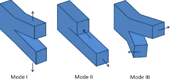
In a homogeneous material, the analytical expressions for the stress and displacement field components provided by LEFM include a multiplying factor, known as the stress intensity factor, which depends on the external stress, the crack length and the geometry of the considered structure, and is related to the energy release rate. The stress intensity factor can be different depending on the considered mode of fracture. There are three basic modes of fracture, which are depicted in Figure 3. Mode I designates the tensile opening mode, which is characterized by the symmetric separation of the crack walls with respect to the plane formed by the crack axis and crack front. Mode II, also called the in-plane sliding mode, is described by a shear stress parallel to the crack plane and perpendicular to the crack front. In mode III, also known as the tearing or anti-plane shear mode, the shear stress acts in the crack plane and parallel to the crack front. In real problems, cracks are usually found to open in mixed modes.

Figure 3: Illustration of the three fracture modes.

The expression of the stress field components in the vicinity of the crack-tip lying in a homogeneous linear elastic medium for a specific mode of fracture can be written as in [66] as

(25)

9 𝜎𝑖𝑗 = 𝐾 √2𝜋𝑟𝑓𝑖𝑗(𝜃) + ∑ 𝐵𝑚𝑟 𝑚 2_𝑔_𝑖𝑗(𝑚)_(𝜃) ∞ 𝑚=0 , (1)

where 𝐾 is the stress intensity factor for the considered mode, 𝑓𝑖𝑗 is an angular function, 𝐵𝑚

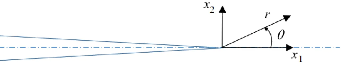
and the dimensionless function 𝑔_𝑖𝑗(𝑚) respectively designate the stress-dependent coefficient and a trigonometric function for the 𝑚𝑡ℎ term. The quantities 𝑟 and 𝜃 are the polar coordinates, for which the origin is placed at the crack tip as illustrated in Figure 4. The indices 𝑖 and 𝑗 are taken in {𝑥, 𝑦} to obtain the expression of the stress field components in a Cartesian base, whereas if a polar base is considered, then 𝑖, 𝑗 ∈ {𝑟, 𝜃}. A representation of the stresses in these two different bases is given in Figure 4. At a sufficiently small distance from the crack tip, the high-order terms of the right hand side of Eq. (1) are negligible with respect to the first one. In this condition, the stress can be assumed to vary as 1/√𝑟. In case of an infinite plane containing a 2𝑎₀long crack opening in mode I, 𝐾 = 𝜎_𝑦𝑦∞_{√𝜋 𝑎}

0, where 𝜎𝑦𝑦∞ is

a tensile stress applied remotely and perpendicular to the crack surfaces.

Figure 4: Illustration of the two-dimensional stress in different coordinate systems and bases in the vicinity of a crack tip.

For a linear elastic medium, Hooke’s law provides a linear relation between the strain tensor 𝜀𝑖𝑗 and the stress tensor as

𝜀_𝑖𝑗 = 𝑠_{𝑖𝑗𝑘𝑙} 𝜎_𝑘𝑙 or 𝜎_𝑖𝑗 = 𝑐_{𝑖𝑗𝑘𝑙} 𝜀_𝑘𝑙 (2)

where 𝑠_{𝑖𝑗𝑘𝑙} and 𝑐_{𝑖𝑗𝑘𝑙} are the compliance tensor and the stiffness tensor respectively. By considering small deformation, the strain tensor is connected to the displacement field 𝑢𝑖

through the expression

𝜀𝑖𝑗 = 1 2( 𝜕𝑢_𝑖 𝜕𝑥𝑗 + 𝜕𝑢𝑗 𝜕𝑥𝑖). (3)

The out-of-plane stress and strain are affected by the considered plane-state condition. The plane stress state is suitable to represent mechanical problems occurring at the surface (or near surface) of thick bodies or in thin media as the stress components relative to the out-of-plane direction is zero. In contrast, the plane strain state is suited to represent mechanical problems taking place within the volume of a thick body as the strain components relative to the

(26)

out-of-10

plane direction are zero. In summary, in plane stress 𝜎_𝑧𝑧 = 0 and 𝜀_𝑧𝑧= −𝜈(𝜎_𝑥𝑥+ 𝜎_𝑦𝑦)/𝐸 and in plane strain, 𝜎_𝑧𝑧 = 𝜈(𝜎_𝑥𝑥 + 𝜎_𝑦𝑦) and 𝜀₃₃= 0, where 𝜈 and 𝐸 are the Poisson’s ratio and the Young’s modulus.

Considering fracture in mode I, the angular functions of Eq. (1) for an isotropic and linear elastic body in a Cartesian base are expressed as [66],

𝑓𝑥𝑥(𝜃) = cos 𝜃 2[1 − sin 𝜃 2sin 3𝜃 2], (4) 𝑓_𝑦𝑦(𝜃) = cos𝜃 2[1 + sin 𝜃 2sin 3𝜃 2], (5) 𝑓_𝑥𝑦(𝜃) = sin𝜃 2cos 𝜃 2cos 3𝜃 2 . (6)

The associated displacement field for such body is given as

𝑢_𝑥 =𝐾𝐼 (1 + 𝜈) 𝐸 √ 𝑟 2𝜋cos 𝜃 2[𝜅0− 1 + sin2 𝜃 2], (7) 𝑢_𝑦 =𝐾𝐼 (1 + 𝜈) 𝐸 √ 𝑟 2𝜋sin 𝜃 2[𝜅0+ 1 − cos2 𝜃 2], (8)

where 𝜅 = 3 − 4 𝜈 in plane strain and 𝜅 = (3 − 𝜈)/(1 − 𝜈).

A description of the anisotropic linear-elastic stress field in proximity of a crack tip has been developed by Paris and Sih [67]. According to their theory, for anisotropic and homogeneous bodies undergoing a fracture in mode I, 𝜎_𝑖𝑗 can be expressed through the use of Eq. (1) with

𝑓_𝑥𝑥(𝜃) = Re { 𝜇1𝜇2 𝜇₁ − 𝜇₂( 𝜇2 √cos 𝜃 + 𝜇2sin𝜃 − 𝜇1 √cos 𝜃 + 𝜇1sin𝜃 )} , (9) 𝑓_𝑦𝑦(𝜃) = Re {_𝜇 1 1− 𝜇2( 𝜇1 √cos 𝜃 + 𝜇2sin𝜃 − 𝜇2 √cos 𝜃 + 𝜇1sin𝜃 )} , (10) 𝑓_𝑥𝑦(𝜃) = Re {_𝜇𝜇1𝜇2 1− 𝜇2( 1 √cos 𝜃 + 𝜇1sin𝜃 − 1 √cos 𝜃 + 𝜇2sin𝜃 )}, (11)

where Re is the real part of a complex number, and 𝜇1 and 𝜇2 are the conjugate pairs of roots

of

𝑆11 𝜇4− 2𝑆16 𝜇3+ (2𝑆12+ 𝑆66) 𝜇2− 2𝑆26𝜇 + 𝑆22 = 0. (12)

When 𝜇1 = 𝜇2 , the stress field relations boils down to the isotropic ones. The

(27)

11 [ 𝜀_𝑥𝑥 𝜀_𝑦𝑦 2𝜀_𝑥𝑦] = [ 𝑆11 𝑆12 𝑆16 𝑆12 𝑆22 𝑆26 𝑆₆₁ 𝑆₆₂ 𝑆₆₆] [ 𝜎_𝑥𝑥 𝜎𝑦𝑦 𝜎𝑥𝑦 ], (13)

and are combinations of the three-dimensional compliance components 𝑠_{𝑖𝑗𝑘𝑙}. The displacements in the vicinity of the crack tip can subsequently be deduced by using Eqs.(9)-(13).

3.2 Interface cracks

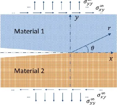
An interface between two solids of dissimilar material is commonly a low-toughness fracture path in various materials. A number of investigations about the crack-tip fields in bi-material interface crack problems, as that illustrated in Figure 5, have been carried out in the previous century [68, 69, 70, 71, 72, 73, 74, 75, 76]. An outcome of these studies is the formulation of analytical expression for a two-dimensional near crack-tip stress field as [76],

𝜎𝑖𝑗 =

1

√2𝜋𝑟 [Re(𝐾

∗_𝑟𝐽𝜔_{) 𝛴}

𝑖𝑗I + Im(𝐾∗ 𝑟𝐽𝜔) 𝛴𝑖𝑗II] , (14)

where 𝑖, 𝑗 ∈ {𝑥, 𝑦}, 𝐽 is the complex number, i.e. 𝐽 = √−1, and the tensors components 𝛴_𝑖𝑗𝐼 and 𝛴_𝑖𝑗𝐼𝐼 are the angular functions, whose expressions can be found in polar coordinates in [76] and in Cartesian coordinates in [77]. The oscillatory parameter 𝜔 is defined as

𝜔 = 1

2 𝜋ln [ 1 − 𝛽0

1 + 𝛽₀] , (15)

where 𝛽₀ is a Dundurs parameter and is expressed as [78], 𝛽₀ = 𝜇1(𝜅2− 1) − 𝜇2(𝜅1− 1)

𝜇₁(𝜅₂+ 1) + 𝜇₂(𝜅₁+ 1) , (16)

where 𝜇𝑖 (𝑖 = 1,2) is the shear modulus in the material 𝑖, assumed elastic and isotropic, as

depicted in Figure 5, and 𝜅_𝑖 = 3 − 4 𝜈_𝑖 in plane strain and 𝜅_𝑖 = (3 − 𝜈_𝑖)/(1 − 𝜈_𝑖) in plane stress. The parameter 𝜈_𝑖 is the Poisson’s ratio in the material 𝑖. The parameter 𝐾∗ is named complex interface stress intensity factor as can be seen as a substitute to the mode-I and mode-II stress intensity factors in case of a crack lying in a homogeneous material [79]. At the right hand tip of an isolated crack of length 2𝑎₀ lying along the interface between two semi-infinite planes subjected to remote stresses 𝜎𝑦𝑦∞ and 𝜎𝑥𝑦∞ as displayed in Figure 5, the

complex stress intensity factor can be written as [76], 𝐾∗ _{= (𝜎}

𝑦𝑦∞ + 𝐽𝜎𝑥𝑦∞)(1 + 2 𝐽 𝜔)√𝜋 𝑎0 (2 𝑎0)−𝐽𝜔 . (17)

The term 𝐾∗ 𝑟𝐽𝜔 in Eq. (14) oscillates with 𝑟 for 𝑟 → 0. This results in possible zones of contact or interpenetration for sufficiently small 𝑟. This oscillatory problem has been studied over the years and a review on the topic is provided in [80]. Rice et al. (1990) gives an

(28)

12

estimation of the distance 𝑟_con over which interpenetration or zone of contact takes place [76]. For 𝜔 > 0, 𝑟_con, is expressed through the relation

𝑟con≅ 2 𝐿 𝑒− 𝜓∗_+𝜋

2

𝜔 _, (18)

where 𝐿 is a reference length and 𝜓∗ is the phase angle of 𝐾∗ 𝑟𝐽𝜔. For 𝜔 < 0, the parameter 𝜔 must be change into −𝜔 and 𝜓∗_{into −𝜓}∗_.

Figure 5: Geometry of an interface crack.

Rice et al. (1990) states that the formulation using complex interface stress intensity factor can be considered valid if the range of 𝑟 considered in an analysis is small compared to a reference length, such as the crack length, and sufficiently large compared to the near crack-tip contact zone. For many combinations of materials, 𝑟_con can be subatomic, e.g. it can be smaller than an atomic spacing for a few millimeter-long crack.

(29)

13

4 Introduction to phase-field theory

Material processing, including solidification, solid-state precipitation and thermo-mechanical processes, is the origin of the development of material microstructures. The latter generally consists of assemblies of grains or domains, which vary in chemical composition, orientation and structure. Characteristics of the microstructure such as shape, size and distribution of grains, impurities, precipitates, pores and other defects have a strong impact on the physical properties (e.g. thermal and electrical conductivity) and the mechanical performance of materials. Therefore, the study of mechanisms causing microstructural changes appears necessary to predict the modifications of material properties and, thus, take action to avoid associated malfunctioning components or failure of structures.

Conventionally, the physical and thermodynamic mechanisms acting in an evolving microstructure such as heat diffusion and impurity transportation are modeled through the use of time-dependent partial differential equations and associated boundary conditions. This is, for instance, the case in sharp-interface approaches, where the interfaces between the different microstructure areas are represented by a discontinuity, as shown in Figure 6a, and their positions need to be explicitly followed with time. However, some phenomena are not suitable for sharp-interface modeling when they are combined with other effects [81]. In addition, complex morphologies of grains are hard to represent mathematically by the sharp-interface approaches when the sharp-interfaces interact with each other during phase transformation, e.g. interface merging and pinch-off within coalescence and splitting of precipitates. Moreover, such modeling is found to be more computationally demanding than diffuse-interface approaches. Therefore, sharp-diffuse-interface models are often more appropriate for one-dimensional problems or simple microstructural topologies [11, 82].

(a) (b)

Figure 6: Illustration of (a) a sharp interface and (b) a smooth interface.

An alternate way to describe the microstructure evolution is to use phase-field methods (PFM), which also employ kinetics equation. This type of modeling provides a continuous and relatively smooth description of the interfaces, as illustrated in Figure 6b. The microstructure is represented by variables, also called phase-field variables, which are continuous through the interfaces and are functions of time and space. Thus, unlike sharp interface models, the position of the interface is implicit and determined by the variation of

(30)

14

the variable value. Moreover, no boundary conditions are necessary inside the whole system except at the system boundary. Initial conditions are, however, still required. Consequently, PFT allows not only the description of the evolution of simple but also complex microstructural topologies unlike sharp-interface problems. For instance, the dendritic solidification with its complex features was successfully modeled through the use of PFM [83, 84].

Lately, phase-field modeling has found numerous applications in magnetism and material science processes such as solidification, solid-state phase transformation, coarsening and grain growth, crack propagation, dislocation dynamics, electro-migration, solid-state sintering and processes related to thin films and fluids. A number of these achievements, and comprehensive descriptions and reviews of phase field modeling can be found in [11, 82, 85, 86, 87, 88, 89]. More recent publications show that PFM is a current research field when it comes to modeling phenomena which involve some of the mechanisms listed in this paragraph [90, 91, 92, 93, 94, 95, 96, 97, 98, 99].

4.1 The phase-field variables

In PFT, a microstructural system is described through the use of single or multiple phase-field variables. Depending on the type of quantity it is connected to, a phase-field variable can be conserved or non-conserved. Conserved variables customary refer to local composition quantities, e.g. the concentration or the mass of chemical species. They can also be associated with density and molar volume [87]. According to Moelans et al. (2008), the non-conserved phase-field variable category contains two groups of variables 𝜙: the phase-fields and the order parameters [82]. Both groups are utilized to distinguish two concurrently prevailing phases. The phase-fields are phenomenological parameters indicating the presence of a phase at a specific position and the order parameters designate the degree of symmetry of phases, potentially giving information about the crystallography of a crystal or precipitate and its orientation. However, this distinction is often not made. Thus, conserved and non-conserved phase-field variables can often be found to be respectively termed conserved and non-conserved order parameters [11, 87, 100]. When both non-conserved and non-non-conserved variables are employed, they are usually found coupled in the bulk free energy of the system, especially for diffusional transformations.

In the theory suggested by Landau, the Landau theory, a bi-phase system may be defined by the presence of an ordered phase and a disordered phase depending on their degree of symmetry. The coexisting phases are associated with specific values of the non-conserved order parameter 𝜙, e.g., traditionally, 𝜙 = 0 for the disordered phase and 𝜙 ≠ 0 for the ordered phase [101]. Depending on the formulation, the phase variable can be arbitrarily defined with different values accounting for the different phases of a system. For example, an unstable disordered phase can be designated by 𝜙 = 0 while a stable disordered one is defined by 𝜙 = −1 or +1 [82]. In [102], 𝜙 = −1 accounts for an empty space and 𝜙 = +1 denotes a filled space. A one-dimensional example of the variation of a phase-field variable through an diffuse interface is illustrated in Figure 6b. Therein, phases α and β are associated

(31)

15

with 𝜙 = −1 and 𝜙 = 1 respectively, while the interface is described by the intermediate values of the phase-field variable.

The conserved phase-field quantity is usually a scalar, but the non-conserved variable can be employed as a vector. When used as a scalar, it can be considered a spatial average of its vector form [11]. It is common to use the components of the non-conserved order parameter vector to represent the crystallography and orientation of the phases [103, 104]. Nevertheless, several non-conserved phase-field components can also be used to account for the transitions between the phases in a multi-phase system.

4.2 Minimization of the free energy of a system

4.2.1 The total free energy

In nature, systems strive to find equilibrium by minimizing their energy. In phase-field theory, the evolution of a microstructure, e.g. a phase transformation, is governed by kinetic equations based on the minimization of the total free energy F. The total free energy of the system can be expressed as the sum of characteristic free energies, which are functions of time, space, pressure, temperature and the phase-field variables. The total energy commonly boils down to

F= ∭ ψ 𝑑𝑉 = F_{𝑏𝑢𝑙𝑘}+F_{𝑔𝑟𝑎𝑑}+F_𝑒𝑙 + ⋯ , (19)

where F_{𝑏𝑢𝑙𝑘} = ∭ ψ_{𝑏𝑢𝑙𝑘}𝑑𝑉 is the bulk or chemical free energy and 𝑉 is the volume of the system. The bulk free energy density ψ𝑏𝑢𝑙𝑘 typically takes the form of a double well, which in

the Landau theory is called Landau potential or Landau free energy density. The gradient free energy F_{𝑔𝑟𝑎𝑑} is related to the interfacial energy and accounts for the presence of interfaces through Laplacian terms. The bulk free energy and gradient free energy can be regrouped in a single term, the structural free energy F_𝑠𝑡𝑟 [105]. The elastic-strain free energy F_𝑒𝑙 represents the energy stored by a system subjected to stresses or undergoing elastic deformation. The energy associated with a microstructural swelling or dilatation due to phase transformation can be reflected in the elastic-strain energy term as in [82] or in an extra energy term, e.g. the interaction energy in [106]. Finally, other free energy terms can be added to the expression, such as free energies related to electrostatics and magnetism. Generally, in phase-field modeling, F is employed to characterize the thermodynamic properties of a system and it is not systematically specified as Gibbs or Helmholtz free energy [82].

4.2.2 The bulk free energy density

Originally, the Landau theory was developed to describe phase transformations at a critical temperature 𝑇𝑐 through the use of a thermodynamic potential, the Landau potential. The latter

can be written in terms of pressure 𝑃, temperature 𝑇 and an order parameter 𝜙 (or a combination of several order parameters reflecting the symmetry relations between the phases). It was suggested by Landau that it can be formulated as a polynomial expansion in power of 𝜙 as [101],

(32)

16

ψ_{𝑏𝑢𝑙𝑘}(𝑃, 𝑇, 𝜙) = ψ_{𝑏𝑢𝑙𝑘}(𝑃, 𝑇, 𝜙 = 0) + ∑𝐷𝑛(𝑃, 𝑇)_𝑛

𝑁

𝑛=1

𝜙𝑛_, ₍₂₀₎

where 𝐷𝑛 denotes the nth coefficient of the phase-field variable or order parameter and can be

a function of pressure and temperature. In this paper, the pressure 𝑃 is assumed constant in all descriptions. For the case of Landau’s theory, it is assumed that 𝐷₂ = 𝑎₀(𝑇 − 𝑇_𝑐) where 𝑎₀ is a phenomenological positive constant, 𝑇 is the material temperature and 𝑇_𝑐 is the phase transition temperature. The Landau free energy can be chosen to be symmetric, for instance, in case of a simple bi-phase system characterized by a symmetric phase diagram, but can also be non-symmetric, for example, in case of a gas-liquid transition or system with a phase diagram including a critical point [11].

When using a fourth-order Landau potential with 𝐷1 = 𝐷3 = 0, 𝐵2 ≠ 0 and 𝐷4 > 0, the

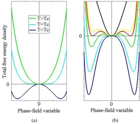
stability of the solid solution, the disordered phase, is traditionally defined by the zero root of the derivative of the system’s total free energy density, while its non-zeros roots characterize the stability of the second phase, the ordered phase. By solely considering the bulk free energy in the total free energy of the system, the prevailing phase is that for which the order parameter values minimize the Landau potential. Thus, in material regions, where the total free energy of the system is similar to that depicted in Figure 7a, the solid solution is stable while the second phase is unstable since there is only one minimum, i.e. for 𝜙 = 0. Figure 7b describes a situation where the second phase is stable and is expected to develop while the matrix phase, unstable, should disappear, i.e. for 𝜙 ≠ 0. With Landau’s formulation, Figure 7a illustrates the appearance of the Landau potential for 𝑇 > 𝑇_𝑐, i.e. 𝐷₂ > 0. The situation displayed in Figure 7b corresponds to an undercooling of a pure solid solution as 𝑇 < 𝑇_𝑐, i.e. 𝐷2 < 0. Thus, the variation of the material temperature can modify the profile of the Landau

potential.

(a) (b)

Figure 7 : Example of a Landau potential profile with (a) 𝑇 > 𝑇_𝑐and (b) 𝑇 < 𝑇_𝑐.

For constant material temperature, the second phase precipitation can be triggered by energy contribution other than F_𝑠𝑡𝑟. In [107], the stress induced by a dislocation, which has an active role in the microstructure evolution, is taken into account by including the elastic-strain free

(33)

17

energy into the total free energy of the system. The gradient of stress in the proximity of the dislocation induces an increase of the transition temperature such that the total free energy density profile changes with distance from the flaw. Thus, second-phase formation can occur in the vicinity of the dislocation, where 𝑇 < 𝑇_𝑐. Away from the defect, 𝑇 > 𝑇_𝑐 and, therefore, the solid solution remains stable. The shift of the transition temperature causes a modification of the total free energy density profile as that illustrated in Figure 8a for a symmetric sixth-order Landau potential.

(a) (b)

Figure 8 : Total free energy of a system omitting the gradient term and including a symmetric 6th order Landau potential to capture. (a) second-order transitions (𝐷4 > 0), and

(b) first-order transitions(𝐷4 < 0).

In other phase-field formulations, the bulk free energy density can be written as in Eq. (20), where the coefficients 𝐷𝑛 are constant. A typical example of a fourth-order Landau

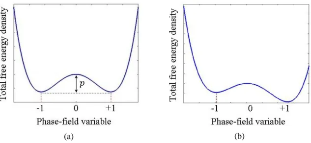
polynomial with 𝐷₄ > 0 is ψ𝑏𝑢𝑙𝑘 = 𝑝 (− 1 2𝜙2 + 1 4𝜙4) , (21)

where 𝑝/4 is the height of the double well or nucleation energy barrier, which needs to be overcome to allow phase transformation [82], and 𝜙 is a scalar phase-field variable. With this example, 𝜙 = −1 and 𝜙 = 1, the minima of the function, can be chosen to represent the existence and stability of two distinct material phases, e.g. the metallic solid solution and a second phase. In absence of F_{𝑔𝑟𝑎𝑑}, the total free energy density of a system defined in this manner has a double-well shape, as illustrated in Figure 9a-b. In the situation depicted by the Figure 9a, the total free energy density of the system is symmetric, i.e. the minima have the same values, and, therefore, both phases can coexist in the microstructure. Figure 9b presents

(34)

18

a situation, where the global minimum is obtained for 𝜙 = 1 and indicating the prevalence of the second phase over the solid solution. The domination of the matrix phase and the second phase over one another can also be caused by the addition of non-symmetric energy terms in the total free energy functional. For example, in [102], the elastic-strain energy includes first and third order terms, which modify the double-well shape by breaking its symmetry.

(a) (b)

Figure 9 : Example of the total free energy density of a system, (a) where the solid solution and the precipitate can coexist, and (b) where the second-phase prevails over the matrix phase. The gradient free energy density term is neglected.

4.2.3 First- and second-order transitions

First-order transitions are characterized by a discontinuous derivative of the system free energy with respect to a thermodynamic variable and a release of latent energy and nucleation of a metastable state of the matter is its starting point. In addition, some materials, which undergo such type of transformation, can display a coexistence of multiple phases for many thermodynamic conditions and compositions. Transformation examples such as liquid solidification and vapor condensation are part of the first-order transition category. When analyzing the total free energy density of a system with respect to the phase field variables or order parameters, metastability is indicated by local minima, while stability is represented by global minima. For second-order transitions, the system free energy first derivative is continuous with no release of latent heat with the second derivative of the system free energy of the system being discontinuous. In this case, the transformation is triggered by the presence of thermal fluctuations. This category includes phenomena such as phase separation of binary solutions, spinodal decomposition in metal alloys or spontaneous ferromagnetic magnetization of iron below the Curie temperature [11].

Depending on the formulations, the use of a fourth-order Landau expansion can allow to capture either first- or second-order transformation [108]. Double-well potentials expressed as in Eq. (20) with 𝐷4 > 0 and Eq. (21), are suitable to modeled first-order transition when

non-symmetric terms are added, see Figure 9. It is also possible to utilize a non-symmetric fourth-order polynomial defined as in the Landau theory to capture first-order transition by taking 𝐷4 < 0.

(35)

19

The addition of higher order terms is necessary to overcome this limitation. Second-order phase transformations are commonly accounted for by using a symmetric fourth-order Landau potential, as defined in Landau theory with 𝐷₄ > 0, see Figure 7. Both order transitions can be modeled by using a higher-order Landau potential as in [107], where a symmetric sixth-order polynomial is employed, with 𝐷₁ = 0, 𝐷₃ = 0 and 𝐷₅ = 0 considering Eq. (20). A system free energy density, which includes such a sixth-order free energy density, is presented in Figure 8a and Figure 8b. In this case, 𝐷6 > 0, which ensures the stability of the system,

𝜙 = 0 designates the disordered phase and 𝜙 ≠ 0 represents the ordered phase. First-order transformations are regarded when 𝐷₄ < 0 while second-order transitions are considered for 𝐷4 > 0. In Figure 8a and Figure 8b, the lower the curves the larger the material transition

temperature or the lower the material temperature. With this formulation, both phases may coexist when the minima of the system’s total free energy have the same value. For example, this can occur for 𝐷₄ < 0, as displayed by the red curve in Figure 8b.

4.2.4 Multi-phase and multi-order-phase systems

In order to account for the energy of a multi-phase system, the bulk free energy density can be constructed with more phase-field variables or components than in the formulations presented above. Thus, various aspects and quantities such as the concentration of solute, the existence of phases, their crystallography and orientation can be represented [82]. For example, the evolution of a multi-phase microstructure can depend on the variation of the concentration of 𝑁 components (𝑐₁, 𝑐₂, … , 𝑐_𝑁) and on the degree of symmetry of the different phases represented by 𝑃 non-conserved order parameters (𝜂₁, 𝜂₂, … , 𝜂_𝑃). As the amount of considered phases-field variables increases, the number of kinetics equation to be solved and their complexity increases. Thus, more computational resources are required to capture the evolution of multi-phase systems.

4.2.5 The kinetic equations

The evolution of the microstructure is steered by kinetic equations, as mentioned in section 4.2.1. The Cahn-Hilliard (CH) equation is employed to govern the evolution of conserved phase-field variables [109] while the time-dependent Ginzburg-Landau (TDGL) equation, also known as Allen-Cahn equation [110], is commonly utilized to model the evolution of non-conserved phase-field variables. In this framework, the time derivative of a phase-field component is connected to the functional derivative of the total free energy of the system with respect to the same phase-field component and a positive kinetic coefficient. The latter is usually referred to as the diffusion coefficient in case of the CH equation and mobility coefficient for the TDGL equation. Through this formulation, the kinetic equations minimize the total free energy of the system at all times, and consequently, allow modeling the dynamic evolution of the microstructure towards a state of equilibrium [111]. When multi-component phase-field variables are employed and thermal fluctuations are neglected, the TDGL and the CH equations can be respectively written with tensor notations as

𝜕𝜂_𝑖

𝜕𝑡 = − 𝑀𝑖𝑗 δF

(36)

20 and 𝜕𝜓𝑖 𝜕𝑡 =∇ ∙ (𝐿𝑖𝑗∇ δF 𝛿𝜓𝑗) , (23)

where the parameters 𝐿_𝑖𝑗 and 𝑀_𝑖𝑗 respectively denote the matrices of diffusion and mobility coefficients. When considering quasi-static transformation, the system is in equilibrium. This state is modeled by setting the functional derivative of the system’s total free energy with respect to the phase-field variables to zero.

Phase-field theory, as introduced in the current section, is used to build the models presented in the next sections of the thesis. Three of them are applied to crack-induced precipitation by using LEFM, introduced in section 3.

(37)

21

5 Phase-field models to predict stress-induced

precipitation kinetics

Over the years, models have been developed to study, predict and simulate second-phase nucleation and formation in materials [104, 106, 112, 113, 114, 115, 116, 117, 118]. Some of them are based on PFT and have found applications in hydride formation modeling in a context of HE. Phase-field methods continue being used increasingly for phase precipitation modeling.

Models based on a symmetric fourth-order Landau-type potential cannot always suitably represent first- and second-order phase transitions. In contrast, microstructure changes involving these two types of phase transformation can be conveniently modeled through the use of higher-order polynomials. A symmetric sixth-order Landau potential-based model was presented in [105, 107] and found suitable to study crack- and dislocation-induced second-phase formation. Such models can be used to cost-effectively study precipitation kinetics by taking into account multiple transitions orders without changing the overall formulation. As seen in sections 2.2.4 and 2.2.5, second/third-phase formation can be triggered and enhanced at the grain/phase boundary and in presence of stress concentrators such as opening cracks in a number of materials. The combination of these aspects on precipitation kinetics might be difficult to observe in laboratory. Modeling is a practical and cheap route to study the phenomenon. However, the addition of multiple aspects affecting the microstructure into a formulation can increase its complexity and, consequently, the computational resources required to solve considered situations as highlighted in [104]. Optimization of such formulation, e.g. by the reduction of the number of equations to be solved, can be beneficial in industrial engineering project in terms of time and costs. Additionally, the coupled mechanical and the phase-field aspects of the microstructural evolution are often treated separately and with different computer programs. By using fully coupled methods convergence can be obtained robustly and both aspects can be considered simultaneously [119]. The possibility to use a single mechanical commercial program to account for interdependent multi-physical aspects affecting second-phase formation can be more interesting within industrial engineering considering cost and time efficiency.

In this thesis, for its practicality to model complex microstructures, PFT is chosen to model stress-induced precipitation kinetics. Different approaches are presented to account for the different aspects related to the system configuration and complexity. All models account for stress-induced precipitation driven by the coupling of the phase transformation-induced swelling of the system and the stress. Model 1 is based on Massih and Bjerken’s work [105, 107], in which a scalar structural order parameter is employed. This model is used to study defect-induced second-phase precipitation within a crystal for different sets of sixth-order Landau potential coefficients. The near-crack stress is implicitly incorporated in the mathematical formulation through the use of LEFM relations for isotropic and anisotropic materials. The second and third models have been developed in order to capture stress-induced second- and third-phase precipitation at grain/phase boundaries, by employing a two-component non-conserved phase-field variables and for a uniform and constant concentration of solute. This choice has been made in order to account for phase transformation in

(38)

22

polycrystalline and multi-phase microstructures, e.g. hydride formation occurring preferentially along grain and phase boundaries in a Ti64 microstructure. These models are suited to predict intragranular, intergranular and interphase crack-induced precipitation as LEFM applied to interface cracks is employed and a parameter is introduced to account for the energy of the grain/phase boundary. Anisotropy in terms of elastic constants and dilatation of the system during phase transformation can also be considered with models 2 and 3. With models 1-3, only the phase-field equation needs to be solved numerically as the mechanical equilibrium is taken into account analytically. This allows modelling of second or third-phase precipitation kinetics with numerical efficiency. Model 4 is formulated to model second-phase formation induced by stress by considering a fourth-order double-well and a non-conserved phase-field scalar. With this formulation, the orientation of the forming hydrides perpendicular to the applied stress as mentioned in section 2.2.2 is captured. The numerical approach associated with this model is based on FEM and a fully coupled method by using the commercial program Abaqus. In this thesis, only diffusionless transformations are considered in an early stage of second/third phase formation as diffusional phase changes induced by stress are assumed to be slower for a given concentration of solute. Thus, the phase transformation aspect is accounted for by solely employing the TDGL equation with all models while mechanical equilibrium is represented either analytically or numerically. Furthermore, the same elastic constants are considered for the precipitate and the matrix phase the second-phase forms from for all models for simplicity.

This section gives a description of the models and numerical strategies used in this thesis.

5.1 Model 1: Sixth order Landau potential for crack-induced

second-phase formation modeling

In model 1, 2 and 3, the spatial position of a particle can equally be referred to through a Cartesian or a polar coordinate system. Thus, the position vector 𝑥_𝑖 is either defined by

(𝑥₁, 𝑥₂, 𝑥₃) or (𝑟, 𝜃, 𝑧). In model 1, second-phase precipitation near the tip of a crack opening in mode I in a crystal is considered. The origin is chosen to be located at the crack tip as presented in Figure 10.

Figure 10: Geometry of the system.

In model 1, employed in papers A and B, a non-conserved order-parameter scalar 𝜂 is chosen to describe the evolution of the microstructure such that 𝜂 = 0 designates the matrix or the solid solution and 𝜂 ≠ 0 represents for the second phase.

The total free energy density of the system with a volume 𝑉 is derived from Eq. (19) and becomes