The Effects of Using Results from Inversion by Evolutionary Algorithms to Retrain Artificial Neural Networks

The Effects of Using Results from Inversion by Evolutionary Algorithms to Retrain Artificial Neural

Networks (HS-IDA-EA-00-106)

Gísli Harðarson (a97gisha@student.his.se)

Institutionen för datavetenskap Högskolan i Skövde, Box 408

S-54128 Skövde, SWEDEN

Examensarbete på programmet för systemprogrammering under vårterminen 2000.

The Effects of Using Results from Inversion by Evolutionary Algorithms to Retrain Artificial Neural Networks

Submitted by Gísli Harðarson to Högskolan Skövde as a dissertation for the degree of B.Sc., in the Department of Computer Science.

June 9. 2000

I certify that all material in this dissertation, which is not my own work has been identified and that no material is included for which, a degree has previously been conferred on me.

The Effects of Using Results from Inversion by Evolutionary Algorithms to Retrain Artificial Neural Networks

Gísli Harðarson (a97gisha@student.his.se)

Key words: Artificial neural networks, inversion, evolutionary algorithms

Abstract

The aim of inverting artificial neural networks (ANNs) is to find input patterns that are strongly classified as a predefined class. In this project an ANN is inverted by an evolutionary algorithm. The network is retrained by using the patterns extracted by the inversion as counter-examples, i.e. to classify the patterns as belonging to no class, which is the opposite of what the network previously did. The hypothesis is that the counter-examples extracted by the inversion will cause larger updates of the weights of the ANN and create a better mapping than what is caused by retraining using randomly generated counter-examples. This hypothesis is tested on recognition of pictures of handwritten digits. The tests indicate that this hypothesis is correct. However, the test- and training errors are higher when retraining using counter-examples, than for training only on examples of clean digits. It can be concluded that the counter-examples generated by the inversion have a great impact on the network. It is still unclear whether the quality of the network can be improved using this method.

Table of contents

1

Introduction ...1

2

Background ...4

2.1 Artificial neural networks... 4

2.2 Training an ANN... 6

2.2.1 Back-propagation learning... 6

2.3 Inversion of ANNs ... 7

2.3.1 A mathematical problem... 7

2.3.2 Inversion methods ... 8

2.4 Introduction to evolutionary algorithms... 9

2.4.1 The theory of EAs ... 9

2.4.2 Sharing in evolutionary algorithms... 10

3

Problem description ...12

4

Experiments ...15

4.3 Inverting the ANN by using an EA ... 16

5

Results...17

7.4 Future work ... 25

7.4.1 Similar experiments ... 25

7.4.2 Termination criteria for back-propagation and EA... 25

7.4.3 Other problem domains... 26

7.4.4 Other methods to choose the counter-examples ... 26

7.4.5 Actual change in the ANN between epochs ... 26

7.4.6 Different inversion algorithm ... 26

References...27

Introduction

1 Introduction

In this report it will be considered if using the results from an inversion of an artificial neural network mapping improves the performance of the network. The idea is to train the network, then invert it and retrain it on input patterns extracted by the inversion. The effect of using the patterns extracted by the inversion will be measured and compared to using random patterns during the retraining. The problem domain that will be considered is recognition of handwritten digits. This domain has also been used in [Lin89], [Jac98] and [Jac00].

1.1 Inversion of ANNs

Artificial neural networks (ANNs) [Rus95] are built on the similar, but very simplified, principles of the human brain. The brain consists of a net of nerve cells that send electrical signals to each other. Likewise, an ANN is based on units that send signals between each other. Much like humans learn by observing their environment, ANNs learn from interaction with the environment. Therefore, ANNs can be used to create solutions for problems that are otherwise difficult to formalise. In many cases it has been shown that ANNs are able to do so. One example is NET-talk, an ANN that learned to map written text in English to pronunciation symbols [Sej87]. A problem that is hard to formalise can often be solved by using an ANN. When using an ANN, the programmer does not create the solution, but feeds examples of input and output patterns to the ANN and lets it adjust itself to map those examples. This is done by using a learning algorithm for the ANN. After training the ANN on these training examples, it will, given that the training was successful, correctly map other input patterns, which are similar to the patterns it was trained on, to the correct output pattern. That is, the ANN is capable of finding the correct output to previously unseen input patterns. ANNs are often used to classify the input examples into specific classes. Creating a function without having to formalise it, leads to that other kind of problems can be solved using ANNs than only using traditional programming.

To be able to use an ANN to solve a problem, a number of problem instances must first be encoded to a set of input-output examples called training set. These examples are then fed to the input nodes of the ANN. The ANN then uses these inputs to create an output represented by the activation of the output nodes. This output should be similar to the output of the corresponding example. After training there is no guarantee that the ANN maps or classifies all possible inputs correctly. Even if thorough tests of the ANN do not indicate any incorrect behaviour, there may still be

Introduction

would not be launched at the wrong time since the cross-validation would have to cover all possible input patterns to do that. The ANN maps a function from a very large or infinite set of input patterns to a set of two output classes, “launch” and “no launch”. When using cross-validation, one input is checked at the time and each pattern has to be tested individually. The size of the set of inputs patterns can make it impossible to test all possible input patterns using cross-validation. Therefore there is a risk that some incorrectly mapped input pattern will not be tested. Instead the question could be asked: “Under what circumstances will the ANN fire?” and then verify that these are the correct circumstances. This is what inversion of the ANN mapping does. It brings out which input patterns the ANN maps to a given output. A few different methods to invert ANNs exist. But since the function of the ANN is not directly invertible, searching methods like gradient descent [Kin90] and evolutionary algorithms [Gol89] can be used to search for inputs that map a given output. These methods are not dependent on whether the function mapped by the ANN is invertible, they just search for an input that gives the desired output. Some inputs may give an incorrect reaction by the ANN and inversion can help finding these inputs.

The reason evolutionary algorithms (EAs) are used in this work is to be able to compare it to [Jac98] and [Jac00]. EAs give a population of candidate input patterns, in contrast to gradient descent search, which only gives a single pattern. The many patterns created by an EA can be spread around in the search space, which increases the chance of finding situations where the system makes an incorrect decision, if there are any such situations. If only one pattern is found, like with gradient descent, this pattern might not be crucial. The algorithm might be stuck in a local optimum.

In general, the inversion of a fully trained ANN often reveals that the ANN incorrectly maps an input pattern to be a typical member of some class, when it really belongs to another class. That is, the ANN would categorise an element outside of a given set to be one very typical member of the set.

1.2 The

hypothesis

The hypothesis of this project is that using the results from inversion of an ANN can improve the mapping of the ANN. The generated inputs by the inversion will be inserted into the training set and the ANN will then be retrained on this expanded training set. Adding these examples to the training set requires a way of knowing whether the generated inputs are the expected patterns, or if they should be categorised as examples of another class, e.g. noise or garbage. In the case a generated input should be considered something other than the expected digit, it can be used to teach the ANN that this is not a typical member of the class, i.e. using it as a

counter-example in the training set.

The reason why these inputs should be used as counter-examples, instead of any randomly chosen inputs, is that the ANN maps these inputs as typical for some class of outputs they do not belong to. Therefore, these inputs should be the counter-examples contributing most to the learning process. This is like teaching a child how to read and write. First the child is given a set of letters and told what each symbol represents and how it is pronounced. Then the process is inverted, i.e. the child is asked how a particular letter looks like and what its characteristics are. If the child answers incorrectly, then the child is corrected so that it can do better next time it is asked. This is the same procedure as will be tested on an ANN in this work.

Introduction

To see if extending the training set with the results from the inversion and retraining the ANN improves the mapping, some measurements and comparison must be made. The error of the test set before and after retraining will be measured to see if the ANN generalises to unseen data better after retraining. The weight-updating rate will be measured during training with the extended training set and this will be compared to adding just random patterns to the training set. This will show whether the inputs generated by the inversion improve the mapping faster than random patterns. The ANN will be trained for a predetermined period of time and then inverted to find counter-examples. The ANN will then be retrained using the training set and the counter-examples. After some time, the ANN will be inverted again to choose new counter-examples. This will be repeated a few times and the effects will be measured.

1.3 Contents

The next chapter contains a background to artificial neural networks, how they are trained, and inversion of such networks. The basic idea behind evolutionary algorithms is explained and the ideology of sharing is introduced.

In Chapter 3, a thorough description is given of the problem domain used in this work. There is a description of what will be tested and how the results will be measured. Finally there is a small section where the expected results from the experiments are presented.

The experiments are described in detail in Chapter 4. Including design of the ANN, which parameters are used, and how the examples from the inversion are chosen. Chapter 5 consists of the results from the experiments. Here is a lot of data that will be analysed in the following chapter.

In Chapter 6 is the analysis of the results in Chapter 5 and the conclusions that can be derived from the results.

Chapter 7 consists of more discussion about the results and what they may mean, what can be learned from this project, and what can be done to continue the work.

Background

2 Background

This chapter contains a general background to ANNs, inversion of ANNs, and evolutionary algorithms.

2.1 Artificial neural networks

The human brain consists of about 1011 nerve cells [Rus95] that are connected by synapses in a very complex network. There are estimated to be about 1014 synapses [Rus95] in the human brain. Signals are sent to adjacent cells by an electrochemical reaction, and each synapse alters the signal. Some synapses increase the signal and others decrease it. It is believed that learning is due to changes in how the synapses alter the signals.

The principle of the construction of ANNs is the same as for the human brain, i.e. signals are sent between simple units (nodes), although the ANNs are very simplified. A simple ANN is shown in figure 1.

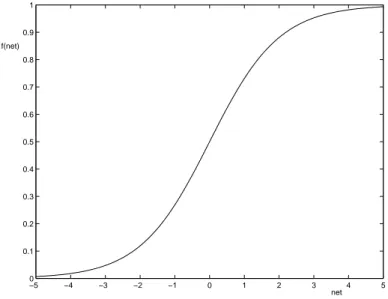
Each connection between nodes has a certain weight, which influences the activation sent between the two nodes, either by increasing it or by decreasing it. Each node basically performs an arithmetic function that gives an output signal based solely on the inputs it gets. First all the incoming signals are added to get the net-value. Then the net-value is used as input into a function that each node uses to make the decision on how strong a signal to send. This function is called an activation function. The output of the node is called its activation and it often has the range from 0 to 1. The S-shaped sigmoid function (see figure 2) is a common activation function [Rus95] and is defined as net e a ₋ + = 1 1 (2.1)

All the incoming activations are multiplied by the intermediate weights to produce the incoming signal. Each node also has a bias weight, which can be seen as a connection

Output nodes Oi

Hidden nodes aj

Input nodes Ik

Figure 1: A two-layer feed-forward network. Bias not shown in figure.

Weights Wj, i

Background

from a node with a constant full activation. The net-value is the sum of all these incoming signals and is the input into the activation function (see figure 3). During the training phase, all the weights, including the bias weight, are fine-tuned by the learning algorithm. Since the bias can be viewed as a weight of a connection from a node that always has full activation, it can be seen as setting the threshold for whether the activation will be high or low.

In this work, a standard feed-forward multilayer network is used, i.e. the nodes are arranged into layers and there are no recurrent connections in the network, i.e. there are no loops where an output from a node is used as an input to a node in a lower layer. A multilayer network creates a mapping from an n-dimensional input space to a typically smaller m-dimensional output space. ANNs have been used for many problems of this kind, e.g. the earlier mentioned NET-talk (see Section 1.1). The mapping often proves to be more or less general, so that the ANN can predict correct out-data from previously unseen in-data. This property is called generalisation. The most usual way to test for generalisation is to use cross-validation where a carefully chosen test set [Rus95], which consists of unseen training examples is run through the ANN and the outputs from the ANN are compared to the correct outputs. A correct generalisation by the ANN of the test set indicates that the ANN has learned a correct mapping.

Figure 2: The sigmoid function, defined in equation 2.1.

−5 −4 −3 −2 −1 0 1 2 3 4 5 0 0.1 0.2 0.3 0.4 0.5 0.6 0.7 0.8 0.9 1 f(net) net

Background

2.2 Training an ANN

The aim of training ANNs is to let the ANN map and generalise a certain function, e.g. from a real world domain like digit recognition. This function is often very complex and it may be very hard to define it explicitly. Instead the ANN can be trained on examples of inputs and corresponding outputs, which is called supervised

learning [Rus95]. A set of training elements is used, where each element is a pair of

an input vector I, and its associated target vector T. Then, to reduce the error of the output, a learning algorithm is used to alter the weights of the ANN. The goal of the training is to minimise the summed square error E of the examples in the training set [Rum86]. The error is defined as

2 , , ) ( 2 1

∑∑

where c is an index of elements in the training set, and j is an index of output nodes.

oj,c is the activation of output node j of the output vector Oc produced by the ANN

when given the input vector Ic associated with the target vector Tc. There is however a problem when training an ANN, which is that usually the training set is incomplete since the number of possible inputs may be very large or infinite. That is, only some of the inputs are used in the training. Nevertheless, since the ANN is able to generalise to unseen data, it might solve the problem.

2.2.1 Back-propagation learning

One of the most popular methods for training multilayer networks [Rus95] is back-propagation learning, a supervised gradient descent training algorithm. Rumelhart, Hinton, and Williams introduced back-propagation learning in 1986 [Rum86]. In short, back-propagation learning attempts to minimize the error of the network by using the derivative of the error, E, to estimate how much each node and each weight contributed to the error of the output. Then the error is propagated back in the network through the weights and the error contribution of the weights is determined. Then the weights are updated in the direction that, according to the derivative, decreases the error. Wn

∑

+

=

w

w

x

net

( )

Figure 3: A computational node and how it calculates the activation [Rus95].

. . .

Background

More precisely, when using the back-propagation learning algorithm, each training example’s input is run through the ANN. The error of the examples in the training set is calculated by equation 2.2.

Then for a every example the error of the output i, is ∂E ∂O_i =T_i −O_i. To see how much the net-value from the previous node contributes to the error, we calculate

( )

i

i E O f net

net

E ∂ =∂ ∂ ⋅ ′

∂ . The error of the weights to output Oi is then

i j j i E net O w E ∂ =∂ ∂ ⋅

∂ , and the simplest way to update the weights is to do it

proportionally to the error of the current weight. The change of a weight, ∆w, is calculated by:

( ) (

)

Where η is the learning rate indicating how much of the error for every example should be corrected every epoch. When the weights connected to the output units have been updated, we propagate the error backwards. That is, it is estimated how much of the error is caused by each node and a new error value is calculated for each node. Then the weights connected to that node are updated the same way as they were in the previous layer (see equation 2.3). This cycle is then repeated until the input nodes have been reached.

2.3 Inversion of ANNs

There are some differences between using a traditional programming approach and ANNs to solve a problem. The traditional programming method consists of an analysis of the problem and a model of the solution, before the program is created. But in the case of ANNs, the programmer does not directly program how the ANN acts on a given input. He must rely on the learning algorithm to successfully do its job. However, such blind faith can be dangerous. Before using an ANN that has been trained, it should be made sure that the ANN gives correct answers under as many circumstances as possible. Doing this requires some sort of an analysis of the behaviour of the ANN. One of these analysis methods is inversion.

Inversion is one way to analyse an ANN’s mapping to see what are the most typical inputs for a given output. In this work an evolutionary algorithm (EA) is used to perform the inversion. The advantages of using an EA are that the EA does not return a single answer but can, using sharing, return a diverse set of input patterns [Gol89] and that they are generally better at avoiding local optima than gradient descent [Gol89]. These properties are relevant since most often multiple inputs give the same

Background

Using mathematical terms this can be written as B-f(A)=∅. For a function f: A→B to be injective, no element in the value set can be a function of more than one element in A, that is f(a1) = f(a2) ⇒ a1 = a2. When a function f is bijective, an inverse function, f -1

: B→A, can be created.

However, when working with an ANN, the function it maps is not mathematically invertible since it maps many inputs to the same output, and is therefore not injective. This problem is avoided by not trying to create an inverse function, but instead for each desired output, to search for the corresponding input pattern.

2.3.2 Inversion methods

ANNs can be inverted in a few different ways. For example another ANN could be used, by training it to do the output to input mapping. Another way is performing gradient descent search to find a pattern that the ANN maps to the given output. A third way is using an evolutionary algorithm as a searching algorithm to find the desired input patterns.

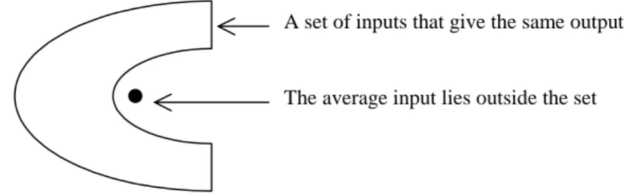
Using an ANN to generate inputs from outputs has some interesting properties. The ANN is then trained by usual methods, e.g. back-propagation, on the same training set, except that outputs become inputs and vice versa. In the case where the original mapping maps many inputs to the same output, the ANN used for inversion is trained on set of data, where the same input produces different output. This causes the ANN to map an input to the average output of that class. In some cases this can be satisfactory, but it can also be that this average output is not a member of the class (see figure 5).

A B

Figure 4: A surjective but non-injective function from A to B. Inverting a function like this would cause each element in B to give two inputs and the inversion would not be defined as a function.

A set of inputs that give the same output

The average input lies outside the set

Background

Gradient descent for inversion of ANNs [Kin90] uses back-propagation input adjustment [Wil86] to search for inputs, which cause the ANN to generate specific outputs. This method is built on the same principles as the back-propagation learning algorithm. Starting with an input, the error from the desired output is calculated and propagated back. But instead of updating the weights and changing the mapping of the ANN, the inputs are altered to minimise the error. This method has a tendency to get stuck in a local optimum [Gol89]. Each search gives one result, and the result depends on where in the input space the search began.

The evolutionary algorithm (EA), which will be described in Section 2.4, uses sharing and usually gives a diverse set of answers, usually manages to avoid local optima [Jac00]. For these reasons, and to be able to compare with the results from [Jac98], an EA will be used to invert the ANN mapping

2.4 Introduction to evolutionary algorithms

2.4.1 The theory of EAs

An evolutionary algorithm (EA) is a search algorithm that follows similar behaviour patterns as evolution in nature, i.e. survival of the fittest [Gol89]. Starting with a random initial population of individuals, the ones that are the most fit are more likely to be chosen for reproduction of individuals for the next generation. To know how well the individuals fit the environment, there must be some way of measuring their fitness. This is done by a fitness-function that reflects the quality of an individual. A high fitness-value means that an individual is well adapted to the environment, and is therefore more suitable for reproduction than an individual with a low fitness-value. The EA described here is a special case and there are several other possible implementations and interpretations. In the EA, individuals are represented by a string of numbers with values from 0.0 to 1.0. The offspring are created by crossover and/or

mutation and then individuals are selected to survive to the next generation. Crossover

is when two individuals mix their internal representation to create offspring. If the strings are of length l, then the crossover is done at the position k, where 0 < k < l. For example, if the strings A=(a1,a2,a3,a4,a5) and B=(b1,b2,b3,b4,b5) are to be combined, crossover at position k=3 would result in two new individuals

A’=(a1,a2,a3,b4,b5) and B’=(b1,b2,b3,a4,a5) [Gol89].

Mutation of individuals happens after crossover. This means that each number in the string is altered from the original value. This can be implemented using different approaches, but in this work the amount each number being mutated changes, follows Gaussian distribution, i.e. most numbers change very little but a few are changed

Background

rest of the new generation is created by crossover of individuals and mutation. Individuals with high fitness-value are more often chosen for reproduction than individuals with low fitness-value. This way, the best individuals are not lost, even though all the offspring might have low fitness.

This cycle of measuring fitness, choosing individuals for reproduction, and creating a new generation goes on until certain criteria are met (see figure 6).

2.4.2 Sharing in evolutionary algorithms

It was shown in [Jac00] that inversion using an EA with sharing gives multiple answers and manages to avoid getting stuck in a local optimum. Sharing is a method used to introduce diversity into the population of candidate solutions [Gol89]. The idea is that the individuals that are alike share resources the way that individuals are penalised for being alike. To give an example of this, lets look at an example where there are two apple trees, and a population of 100 individuals. Tree A gives 100 apples but tree B gives 10 apples. Without sharing all the individuals would eventually gather around tree A since it gives much more apples. With sharing however, if all the 100 individuals were around tree A, they would have to divide the 100 apples between them and only get one apple each. Then it would be better for an individual to be the only one at tree B since that would give the individual 10 apples. That is, the individuals are penalised for being close together. This leads to that not all the individuals gather around the best resource but some find other lower peaks but stay there since there might be overpopulation around the best resource. This helps in finding incorrectly classified inputs of the ANN, since the results from the EA are not just slightly different representations of the same pattern but are likely to be a few different patterns.

Sharing is implemented by a function that gives higher value for individuals that are like each other [Gol89], and is defined by equation 2.4. The function d(xi,xj) gives the distance or difference between two individuals, and s(d) calculates the sharing value:

⎪⎩ ⎪ ⎨ ⎧ ≥ < − = share share share share d if d if d d s σ σ σ σ 0 ) ( (2.4) Evaluation of individual Fitness calculation Fitness-based selection Crossover Mutation Evaluation Population, time t Reproduction Population, time t+1 An individual Figure 6: Overview of an evolutionary algorithm [Gol89].

Background

σshare is the distance that marks how far away two individuals must be to have no sharing. This function gives the sharing value 1 if the distance between two individuals is 0, and when the distance is σshare then the sharing value is 0 (see figure 7).

The new fitness-function using sharing, fs(xi), increases the fitness for an individual that is different from many others (equation 2.5). The value from this function will be used to select individuals for reproduction. The function f(xi) is the old fitness-function that tells how well an individual fits the environment.

( )

( )

(

)

∑

An individual that is different from most of the other individuals gets a low accumulated sharing value and the new fitness-function will be higher than if the individual had a high sharing value. This causes the individuals be spread out in the search space and also decreases the risk of getting stuck in local optima.

Figure 7: The triangular sharing function described in [Gol89]. σshare is the distance that

marks how close individuals must be to be affected by sharing.

1.0

0.0

0 Distance σshare

Share s(d)

Problem description

3 Problem description

The candidate solutions created by the inversion are the inputs that the ANN regards as the most typical inputs for a given output. If these inputs are incorrect, i.e. they are inputs that should generate other outputs than they currently do, then it can be assumed that the ANN critically classifies these inputs erroneously.

As suggested in [Lin89], adding these inputs, along with the correct outputs, as counter-examples, to the training set should therefore have a significant influence when retraining the network, and give a better generalisation of unseen examples. Inverting the ANN in the defence system example (see Chapter 1) could reveal that under some peaceful circumstances, a missile would have been fired. This situation could then be added into the training set as a counter-example for the retraining of the ANN so that the ANN would react correctly in the situation, which it failed to do before.

In this work the ANN will be trained on a realistic but limited problem domain to see if this theory is correct. After training the ANN, it will be inverted in hope of finding incorrect classifications. After adding the results to the training set as counter-examples, the ANN will be retrained. Error measures will be recorded and the ANN will be inverted again to see which effect retraining using the counter-examples has on the ANN. This will be described in more detail in Section 3.2.

3.1 Problem

domains

In this project one problem domain will be considered. It is recognising pictures of handwritten digits, written with black ink on white paper. Here is a problem that it cannot be determined automatically whether the results from the inversion should be categorised as giving the desired output or just some random garbage. The reason for this is that there is no function that can be used to determine what a digit looks like. The perfect digits do not exist, if that were the case, traditional programming methods could be used to solve the digit recognition problem. But since these perfect digits do not exist, the ANN must first learn by examples how the digits are written to be able to determine whether an input pattern can be categorised as a digit or something else.

3.1.1 Digit recognition

The digit recognition problem has been used before by [Kin90], [Jac98], and [Jac00]. Black and white pixel maps of size 8 x 11 pixels are used to represent the image of handwritten digits and the task of the ANN is to recognise the digits. This means that the ANN has 88 inputs and 11 outputs, one for the activation of each digit and one for non-numbers or garbage. If the network classifies a pattern to be the digit “3”, then only the corresponding output nod will have a high activation. The training set consists of 49 examples of each digit. Because the network structure can have significant influence on whether the network is able to generalise to unseen data, or if the network just learns the training set, the same ANN structure as [Kin90] and [Jac00] will be used. The ANN will be described in more details in Section 4.2.

It will be tested whether assuming that all the results from the inversion could be considered as counter-examples and whether adding them to the training set, will reduce the error of the ANN. This introduces the risk of adding some correct input patterns as counter-examples. The hope is that this will not be a problem for the ANN

Problem description

as long as these incorrect training elements are not a dominating number of the whole set. Even though the inversion would give an input pattern that would be considered by a human observer to be a digit, it is likely that it would also have some activation that is wrong. That is, some input patterns would have high activation where they should have low, or vice versa. If these wrong activations exist because the training algorithm did not adjust all the initial weights of the ANN correctly, then adding the generated inputs to the training set as counter-examples would reduce these incorrect activations as it would reduce the correct activations too. However, the examples in the original training set increase the correct activation and therefore adding all the examples as counter-examples, should reduce incorrect activation without having much influence on the correct activation.

3.2

Measurements

For this problem domain, the average error of the elements in the test set will be measured before and after retraining, in hope that it will be lower after each retraining. Error of an element, Ep, can be measured by the Least-Mean-Square-Error [Lin89] as following:

∑

As before, tk is the target output of node k, and ok is the output of node k generated by the ANN. The weight-updating rate, v, as the Euclidian distance in weight space, will also be measured. It is a measurement of how much the weights are updated each epoch. That is |∆W| where ∆W is a vector of all ∆wj,k in the network and ∆wj,k is the change in weight between nodes j and k during learning. The weight-updating will here be defined as:

( )

∑ ∑

Where |T| is the size of the training set, c is an index of examples in the training set, and ∆w is the change of one weight for a given example. A higher value of v indicates a bigger change in the weights for a given epoch, and therefore faster learning by the ANN.

It will also be interesting to see if iterative inversion results in fewer incorrect results. That is, if inverting after retraining using counter-examples, will create patterns that are more like digits than before. This will only be done informally since it is no method available that can be used to say for sure if one pattern is more like a digit

Problem description

The weight updating rate, v, should be higher using input patterns generated by the EA as counter-examples, than only using random patterns. That is the ANN should be quicker to adopt the mapping to fit the training set. This means that counter-examples created by inversion by the EA, should cause more updates of weights during retraining than the random patterns do. The reason for this is that the examples extracted by the inversion are very strongly categorised by the ANN as a digit. By using these examples as counter-examples to what the ANN currently maps them to, the ANN is told to differently map an example that is considered by the ANN to be a typical digit.

Experiments

4 Experiments

4.1 General

overview

Experiments were made to test the hypothesis stated in Section 1.2. First the ANN was trained on set of data for a certain time. Then the ANN was inverted for each output pattern, using an evolutionary algorithm. A part of the results from the inversion was then inserted to the original training set as counter-examples, i.e. categorised as garbage, and not as a number. These examples were only chosen accordingly by the shared fitness value, and no attempt was made to sort out which examples are actual digits. After retraining the ANN with this expanded training set, the same procedure of inversion was made. This was repeated 5 times. For comparison, both EA-generated counter-examples and random counter-examples were used. The whole experiment was then repeated 5 times to generate more reliable results. The average of these results were used for the comparison. Figure 8 shows the outlines of the experiments. For comparison to traditional ANN-training, five experiments with no garbage examples were also run and the average results were used.

Choose new inputs and add them to the training set

(Re-) train ANN - measure mean error - measure v Run EA to invert ANN Done Finished Begin Not done

Experiments

then one garbage output for patterns that do not represent a digit. The weights were initially randomised in the interval [-0.5, 0.5].

4.2.1 The training

The ANN was trained using back-propagation for periods of 2000 epochs. As results of initial experiments, the learning rate was chosen to constantly be 0.05 and the

momentum term was set to 0.75. Momentum indicates how much influence previous

training example has on ∆w. ∆w = ∆wnew + momentum * ∆wold. The basic training set consisted of 49 * 10 digits and the test set consisted of 14 examples of each digit but no garbage patterns.

Training the ANN where no counter-examples were used, was made by training the ANN 10000 epochs on the original training set. In all the experiments, no examples were used during training for the first 2000 epochs. In the cases counter-examples were added, they were chosen in two different ways dependent on the experiment. When using inversion, the 10 best patterns of each digit, according to shared fitness, were chosen from the results from the inversion. The other way was to create randomly chosen patterns, with the same average darkness as the training set. That is, in average 27% of the pixels were black and the rest are white. In both cases the total number of counter-examples is 100. A new set of counter-examples was created every 2000 epochs.

4.3 Inverting the ANN by using an EA

The evolutionary algorithm takes as inputs a network, a target class, population size, elite size, mutation, sharing, and number of generations. Every time an ANN was inverted, all parameters but the target class were kept the same (see Sections 2.4.1 – 2.4.2 for descriptions of concepts).

The population was chosen to be 100 individuals where 20 survived to the next generation. Mutation probability, σ, was 0.01 and sharing was always used. For every inversion the EA ran for 1000 generations.

After every inversion, the 10 best individuals were chosen, according to shared fitness, to be counter-examples in the training for the next 2000 epochs. One inversion for each digit gives totally 100 patterns as counter-examples.

Results

5 Results

This chapter contains the results from the experiments described in Chapter 4.

5.1 Summed Square Error

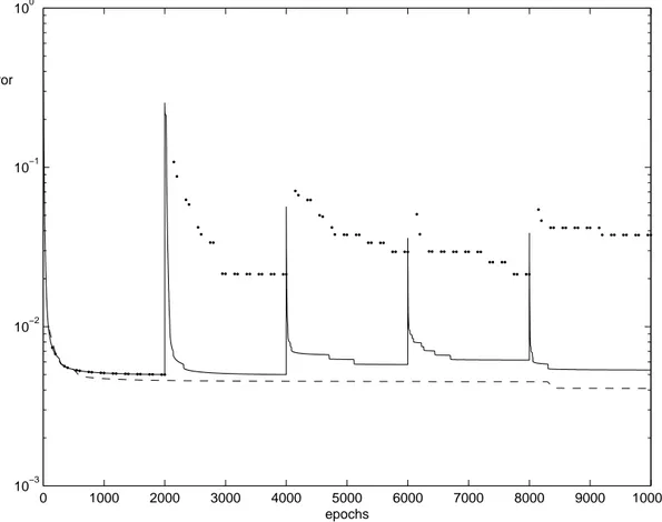
The ANN does not map the training set as correctly when the EA-generated counter-examples have been added, compared to adding random garbage. The lowest error was found with a static training set and without any counter-examples (see figure 9).

Figure 9: The error of the training set. The thick dotted line is when training with counter-examples from the inversion. The thin solid line is training with randomly generated garbage. The dotted line shows the error when training without any counter-examples. 0 1000 2000 3000 4000 5000 6000 7000 8000 9000 10000 10−3 10−2 10−1 100 epochs Error

Results

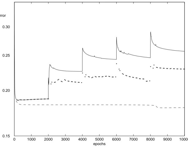
The error of the test set is lower if the EA-generated counter-examples are used than if random examples are used in the training. However, when the counter-examples have been fed to the ANN, it becomes worse at generalising to the counter-examples in the test set, than not using any counter-examples in the training (see figure 10).

0 1000 2000 3000 4000 5000 6000 7000 8000 9000 10000 epochs 0.30 0.25 0.20 0.15 Error

Figure 10: The error of the test set. The thick dotted line is when training with counter-examples from the inversion. The thin solid line is training with randomly generated garbage. The dotted line shows the error when training without counter-examples. Note that this figure is drawn with logarithmic scale.

Results

5.2 The weight updating rate

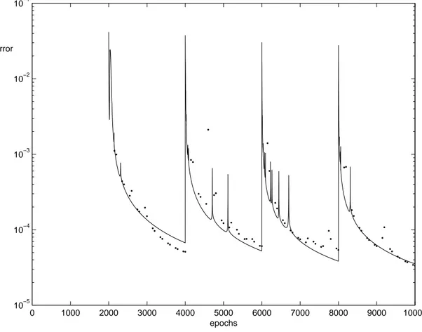
These pictures show how much the weights in the ANN change for each epoch.

The v (from equation 3.2) is generally higher for the EA-generated counter-examples than for the random counter-examples (see figure 11).

Figure 11: Weight-updating rate (v) for each epoch. The thick dotted line is when training with counter-examples from the inversion. The thin solid line is training with randomly generated garbage. This picture shows how much just the additional counter-examples and garbage patterns cause the weights to change.

0 1000 2000 3000 4000 5000 6000 7000 8000 9000 10000 10−5 10−4 10−3 10−2 10−1 epochs Error

Results

Measuring the v for the training set shows that the EA-generated counter-examples cause more updates for the weights than when the counter-examples are created by a random function (see figure 12). The peaks here might be caused by the original training set changing back some of the big change made by the counter-examples just before. This is discussed more in Section 7.1.

0 1000 2000 3000 4000 5000 6000 7000 8000 9000 10000 10−5 10−4 10−3 10−2 10−1 epochs Error

Figure 12: Weight-updating rate (v) for each epoch. The thick dotted line is when training with counter-examples from the inversion. The thin solid line is training with randomly generated garbage. This picture shows how much just the examples in the training set cause the weights to change.

Results

5.3 Iterative

inversion

The Appendix contains some pictures of the individuals that had the highest shared fitness of the final population of each inversion of one experiment. These are the patterns that the ANN classified at that time to be distinctly classified as digits. The different scales of grey represent different amount of activation, where a black pixel represents a strong activation and a white pixel represents no activation. The idea was that iterative inversion would give a pattern that would be closer to what a human observer would categorise as a digit.

The EA was not in all cases able to extract patterns that the ANN classified as a typical digit. These patterns are not shown since they are patterns that the ANN would categorise as something other than the digit that was being inverted.

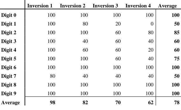
The EA had more problems finding a pattern as the number of inversions increased, and some digits were harder to find than other. shows in percentage how often the EA found a pattern that would be categorised as a digit. All values are averages of five experiments.

Inversion 1 Inversion 2 Inversion 3 Inversion 4 Average

Digit 0 100 100 100 100 100 Digit 1 100 80 20 0 50 Digit 2 100 100 60 80 85 Digit 3 100 40 60 40 60 Digit 4 100 60 60 20 60 Digit 5 100 100 60 40 75 Digit 6 100 100 100 100 100 Digit 7 80 40 40 40 50 Digit 8 100 100 100 100 100 Digit 9 100 100 100 100 100 Average 98 82 70 62 78

Conclusions

6 Conclusions

The results in figure 11 indicate that adding EA-generated counter-examples to the training set of the ANN generally has more effect on the weights during the training phase than adding randomly generated counter-examples, i.e. v is higher for the counter-examples than for the random patterns. This could be because the ANN is told to map a pattern that is currently mapped very strongly into another class. The ANN needs to change its weights more to adjust itself to map these examples correctly, than for random input examples that should be categorized by the ANN as garbage.

What was not expected was that the error of both the training set and the test set, was higher after each retraining. This means that the ANN looses some of its abilities to generalise to unseen data. The error of the training set is higher when adding EA-generated counter-examples than when adding random patterns. One possible reason for this is that some of the counter-examples that were added are actual digits and may therefore push the ANN from its previously successful knowledge about numbers. However, after 2000 epochs, when new counter-examples are added, the error is still getting lower (see figure 9). This means that it takes more time to adjust to these EA-generated counter-examples than it takes to learn the random patterns. The ANN learns to categorise the random patterns faster, since these are far from looking like the digits in the original training set and therefore do not push the ANN as far away from the previous knowledge.

The reason why the error rises after every 2000 epochs (figures 9 and 10) is that the ANN has never seen some of the examples before, and has to learn to categorise them as non-digits. The fact that the error increased this much does not mean that the ANN was bad at generalising before. It is harder to learn to distinct between two patterns that are similar, e.g. a digit and an EA-generated digit, than two patterns that are different, e.g. a digit and a random pattern. Looking at the error of the test set (figure 10), it is clear that even though the error of the training set (figure 9) was higher using EA-generated counter-examples, the test set error is smaller using the EA-generated counter-examples than retraining using random garbage. This indicates that the ANN generalises better to unseen data using the counter-examples from the inversion, than using random patterns as garbage. Retraining using counter-examples, no matter if they are extracted by the inversion or randomly generated, causes the error of both the training set and the test set to be higher than training with no counter-examples at all. It should be noted however, that the test set consisted only of patterns that represented digits, and no patterns that were non-digits. When training using the training set without any counter-examples, the ANN does not learn to categorise anything as garbage. If the ANN were to categorise some garbage pattern without ever seeing garbage in the training set, then it would not know how a garbage pattern looks like and therefore categorise it as some digit. This possibility was not covered in the tests, since the same test set was always used and it had no garbage examples.

According to the tests were it was shown that the error of the test set is lower when retraining with EA-generated counter-examples extracted from inversion than with randomly generated patterns (see figure 10), the ANN appears to generalise better to unseen data and there are bigger changes of the weights, which should minimise the risk that the ANN gets stuck at a local optimum.

Conclusions

It is interesting to see that each time the counter-examples cause a high value of v (from equation 3.2), there is also a peak caused by the original training examples (see figures 11 and 12). This could be because the original training examples adjust back some of the changes caused by the counter-examples. However, corresponding to each peak in v there is also a change in the error of the training set indicating that the ANN has learned some better mapping. The changes in the error of the test are not as obvious, but they also happen the same time as when there are peaks in v.

It is interesting to see that the EA is less successful in finding patterns with high fitness after retraining. shows a summary of numbers, which the EA had problems generating, and the percentage of successful pattern extracted by each inversion. It should be noted how the EA has more problems generating some digits than others. “7” and “1” are only found in 50% of cases while “0”, “6”, “8”, and “9” are always found. This is similar to the results presented in [Jac98] where Jacobsson showed how many generations were needed to find each digit. In his work, the patterns “8” and “9” were found very quickly while “1” and “4” were very hard to find. It is also interesting to see that after the ANN has trained on the counter-examples, the next inversion has more problems finding the patterns. The first inversion nearly always finds a pattern while inverting for the fourth time only manages to do so in 62% of the cases. A reason for this might be that after retraining, the patterns that the ANN maps as a certain digit are so specific, that all the individuals in every generation will be categorised as garbage, and the mutation is not successful in increasing the fitness of the individuals.

Discussion

7 Discussion

7.1 The value of v for the counter-examples and the training set

As has been mentioned before, and can be seen by comparing figures 11 and 12, is that there is a relation between peaks in v (see equation 3.2) for the training set and the counter-examples. Training an ANN using the same training set for a long time causes the ANN to adjust very well to the given examples, and updates of the weights become minimal for every epoch. The ANN has found some optimum in the problem space. When new examples are added to the training set, the ANN has to update its weights again to map the new training set correctly. Each time the counter-examples cause the weights to change, the ANN is no longer in the optimum earlier found for the original training set so the original training set now has more effect on weights than before. It was not measured whether most of the updates by the original training set are changing back the changes made before by the counter-examples (see figure 13).

The length of the vector c is the value of v for the counter-examples and the length of the vector tX is the value of v for the original training set. The actual change in the network is the length of the sum of these two vectors, but that was not measured in this work. This is suggested as a future work in Section 7.4.5

7.2 Relations

between

v and the error of the ANN

Comparison between peaks in the value of v (figure 11) and the decrease of error of the training set (figure 9) shows a direct relation between high value of v and improved mapping by the ANN. Each time the counter-examples cause v to be high it pushes the knowledge of the ANN far from its previous knowledge. This can be seen, as the vector c in figure 13 would be long, since the length of c is the value of v. If the point C (knowledge after training with counter-examples) is far from A (previous

knowledge), then it is more likely that T (knowledge after training with the whole training set) will lie further away from A than if v was small. Decrease in the error of the training set implies that T gives a better mapping than A. However, each big

c t1 t2 A T1 C T2

Figure 13: A visualisation of how training with counter-examples can cause the ANN either to fine tune existing mapping or explore new possibilities. If the current mapping of the ANN is represented by the point A, training with counter-examples causes the current mapping of the ANN to change from A to C. The original training set then either causes the mapping to be TX. T1 represents that most of the updates by the original

training set changes back what the counter-examples changed. The point T2 represents

Discussion

change of the weights does not give reduced error for the test set (figure 10). Sometimes the error increases, which means that even though the ANN becomes better in mapping the training set to the correct outputs, it becomes worse in generalising to unseen data. These changes are, however, minimal.

7.3 Recognising

the

EA-generated digits

Only a part of the EA-generated patterns looks like something a human would categorise as a digit. The hope was that iterative inversion would give patterns that looked more like digits. The fact was that iterative inversion caused the EA to have much more problems in extracting a pattern that the ANN maps as a digit.

A small informal test was made to see if people unfamiliar with these generated digits could categorise them correctly. About 1/3 of the digits were recognised, while 2/3 were recognised by people with some training in reading patterns extracted by the inversion. The pictures used in this informal test were the same kind of pictures as shown in Section 5.3. There did not seem to be any relations between iterative inversion and the percentage of correctly recognised patterns.

7.4 Future

work

To extend this work and better understand these results there are a few things that could be looked at. Firstly there is the possibility to do the same or similar experiments and measure the same things, using different parameters during the tests. The new results could then be compared to the results in this report, to see the effect the various parameters have on the results. Other things to be tested are e.g. other application domains, different methods for choosing which examples to be used as counter-examples, and other methods to invert the ANN.

7.4.1 Similar experiments

The aim of doing experiments similar to the experiments in this project would be to measure the effects of a particular property of either the ANN or the EA.

The ANN could be trained for a different amount of epochs. It might show that training it longer between inserting counter-examples would decrease the error of the network.

An interesting thing would be to change the size of the counter-examples set. More counter-examples for each digit would probably result in higher error and more difficulties for the EA when generating digits, but a higher value of v. Fewer counter-examples would probably have the opposite effects. There might be a trade-off here.

Discussion

found a solution and the fitness has nearly stopped increasing. This could reduce the time that is wasted when training the ANN and the ANN has already learned all it can from the training set. This could also minimise the time spent on inversion after patterns with high fitness have been found.

7.4.3 Other problem domains

Other problem domains should be tested to see if the results represented in this report are dependent on the problem. These problem domains should have very different properties, for example there should exist a well-defined function that can determine whether the patterns from the inversion really are counter-examples. An example of such a problem domain is the 2-problem where the task is to recognise whether binary strings of a fixed length have exactly two active inputs. This problem was studied in [Kin90] and [Jac00] and the results from those experiments can be used for comparison.

7.4.4 Other methods to choose the counter-examples

In this work, the counter-examples were chosen dependent only on the shared fitness. This could cause that all the chosen counter-examples would be alike. A way to see if that is the case, a cluster analysis of the population could be done. Doing so, the population of the EA is grouped according to similarities. It might be enough to choose one or two individuals from each cluster for the retraining.

As a bi-product of this work it could be explored if there exist more than one typical way to write a digit.

7.4.5 Actual change in the ANN between epochs

In Section 7.1 it was discussed how much the actual change of the ANN is. This leads to that it would be interesting to see if the weight update caused by the counter-examples is changed back by the training set. In this project the sum of the changes by each example was measured. Instead, the actual change between epochs could be measured to see if the ANN really changes more using counter-examples extracted by inversion, than for random garbage. The ANN could be checked periodically to see if the changes cause the ANN to “go in circles”.

7.4.6 Different inversion algorithm

Evolutionary algorithms can be quite complex and require much processing power. It is a question whether it is necessary to get a diverse set of counter-examples and local optima avoidance by the EA or if using methods like gradient descent would be as successful. Running gradient descent several times from different start points, might well result in a diverse set of counter-examples.

References

References

[Gol89] Goldberg D. (1989), Genetic Algorithms in Search, Optimization, and Machine Learning, Addison-Wesley

[Jac98] Jacobsson H. (1998), Inversion of an Artificial Neural Network

Mapping by Evolutionary Algorithms with Sharing, Final year

dissertation, HIS-IDA-EA-98-113, University of Skövde, Sweden

[Jac00] Jacobsson H. and Olsson B. (2000), An Evolutionary Algorithm for Inversion of ANNs, In Proceedings of The Third International

Workshop on Frontiers in Evolutionary Algorithms, Wang P. P. (ed.),

pp. 1070-1073

[Kin90] Kindermann J. and Linden A. (1990), Inversion of neural networks by gradient descent, Parallel computing, vol 14: pp. 270-286

[Lin89] Linden A. and Kindermann J. (1989), Inversion of multilayer nets, In

Proc. 1st Int. Joint Conf. on Neural Networks, IEEE, San Diego

[Rum86] Rumelhart D. E., Hinton G. E., and Williams R. J. (1986), Learning representations by back-propagating errors, Nature vol 32:, pp. 533-536

[Rus95] Russell S. and Norwig P. (1995), Artificial Intelligence, a modern

approach, Prentice Hall

[Sej87] Sejnowski T. and Rosenburg C. (1987), Parallel networks that learn to pronounce English text, Complex systems, vol 1: pp. 145-168

Appendix

Appendix

Examples of digits generated by the inversion.

Inversion 1 Inversion 2 Inversion 3 Inversion 4

number 0 − run 1 1 2 3 4 5 6 7 8 1 2 3 4 5 6 7 8 9 10 11 Digit 0 number 0 − run 2 1 2 3 4 5 6 7 8 1 2 3 4 5 6 7 8 9 10 11 Digit 0 number 0 − run 3 1 2 3 4 5 6 7 8 1 2 3 4 5 6 7 8 9 10 11 Digit 0 number 0 − run 4 1 2 3 4 5 6 7 8 1 2 3 4 5 6 7 8 9 10 11 Digit 0 number 1 − run 1 1 2 3 4 5 6 7 8 1 2 3 4 5 6 7 8 9 10 11 Digit 1 number 1 − run 2 1 2 3 4 5 6 7 8 1 2 3 4 5 6 7 8 9 10 11 Digit 1

EA failed in finding the pattern

1 2 3 4 5 6 7 8 1 2 3 4 5 6 7 8 9 10 11 Digit 1

EA failed in finding the pattern

1 2 3 4 5 6 7 8 1 2 3 4 5 6 7 8 9 10 11 Digit 1 number 2 − run 1 1 2 3 4 5 6 7 8 1 2 3 4 5 6 7 8 9 10 11 Digit 2 number 2 − run 2 1 2 3 4 5 6 7 8 1 2 3 4 5 6 7 8 9 10 11 Digit 2

EA failed in finding the pattern

1 2 3 4 5 6 7 8 1 2 3 4 5 6 7 8 9 10 11 Digit 2

EA failed in finding the pattern

1 2 3 4 5 6 7 8 1 2 3 4 5 6 7 8 9 10 11 Digit 2 number 3 − run 1 1 2 3 4 5 6 7 8 1 2 3 4 5 6 7 8 9 10 11 Digit 3 number 3 − run 2 1 2 3 4 5 6 7 8 1 2 3 4 5 6 7 8 9 10 11 Digit 3 number 3 − run 3 1 2 3 4 5 6 7 8 1 2 3 4 5 6 7 8 9 10 11 Digit 3

EA failed in finding the pattern

1 2 3 4 5 6 7 8 1 2 3 4 5 6 7 8 9 10 11 Digit 3

Appendix

Inversion 1 Inversion 2 Inversion 3 Inversion 4

number 4 − run 1 1 2 3 4 5 6 7 8 1 2 3 4 5 6 7 8 9 10 11 Digit 4

EA failed in finding the pattern

1 2 3 4 5 6 7 8 1 2 3 4 5 6 7 8 9 10 11 Digit 4 number 4 − run 3 1 2 3 4 5 6 7 8 1 2 3 4 5 6 7 8 9 10 11 Digit 4

EA failed in finding the pattern

1 2 3 4 5 6 7 8 1 2 3 4 5 6 7 8 9 10 11 Digit 4 number 5 − run 1 1 2 3 4 5 6 7 8 1 2 3 4 5 6 7 8 9 10 11 Digit 5 number 5 − run 2 1 2 3 4 5 6 7 8 1 2 3 4 5 6 7 8 9 10 11 Digit 5 number 5 − run 3 1 2 3 4 5 6 7 8 1 2 3 4 5 6 7 8 9 10 11 Digit 5 number 5 − run 4 1 2 3 4 5 6 7 8 1 2 3 4 5 6 7 8 9 10 11 Digit 5 number 6 − run 1 1 2 3 4 5 6 7 8 1 2 3 4 5 6 7 8 9 10 11 Digit 6 number 6 − run 2 1 2 3 4 5 6 7 8 1 2 3 4 5 6 7 8 9 10 11 Digit 6 number 6 − run 3 1 2 3 4 5 6 7 8 1 2 3 4 5 6 7 8 9 10 11 Digit 6 number 6 − run 4 1 2 3 4 5 6 7 8 1 2 3 4 5 6 7 8 9 10 11 Digit 6 number 7 − run 1 1 2

EA failed in finding the pattern 1

2

EA failed in finding the pattern 1

2

EA failed in finding the pattern 1

Appendix

Inversion 1 Inversion 2 Inversion 3 Inversion 4

number 8 − run 1 1 2 3 4 5 6 7 8 1 2 3 4 5 6 7 8 9 10 11 Digit 8 number 8 − run 2 1 2 3 4 5 6 7 8 1 2 3 4 5 6 7 8 9 10 11 Digit 8 number 8 − run 3 1 2 3 4 5 6 7 8 1 2 3 4 5 6 7 8 9 10 11 Digit 8 number 8 − run 4 1 2 3 4 5 6 7 8 1 2 3 4 5 6 7 8 9 10 11 Digit 8 number 9 − run 1 1 2 3 4 5 6 7 8 1 2 3 4 5 6 7 8 9 10 11 Digit 9 number 9 − run 2 1 2 3 4 5 6 7 8 1 2 3 4 5 6 7 8 9 10 11 Digit 9 number 9 − run 3 1 2 3 4 5 6 7 8 1 2 3 4 5 6 7 8 9 10 11 Digit 9 number 9 − run 4 1 2 3 4 5 6 7 8 1 2 3 4 5 6 7 8 9 10 11 Digit 9