A Benchmark Comparison of Maintenance Policies in a Data Warehouse Environment

A Benchmark Comparison of Maintenance Policies

in a Data Warehouse Environment

Henrik Engström Gionata Gelati Brian Lings

University of Skövde, Sweden University of Modena and Reggio Emilia, Italy1 _{University of Exeter, UK}

henrik@ida.his.se gionata@dbgroup.unimo.it brian@dcs.exeter.ac.uk

Technical Report

HS-IDA-TR-01-005 Department of Computer Science

University of Skövde, Sweden ABSTRACT

A data warehouse contains data originating from autonomous sources. Various maintenance policies have been suggested which specify when and how changes to a source should be propagated to the data warehouse. Engström et al. [Eng00] present a cost-based model which makes it possible to compare and select policies based on quality of service as well as system properties. This paper presents a simulation environment for benchmarking maintenance policies. The main aim is to compare benchmark results with predictions from the cost-model. We report results from a set of experiments which all have a close correspondence with the cost-model predictions. The process of developing the simulation environment and conducting experiments has, in addition, given us valuable insights into the maintenance problem, which are reported in the paper.

1. Introduction

A data warehouse contains data from autonomous sources. When data in sources are updated there is a need to maintain the warehouse views in order to keep them up-to-date. This propagation of changes is commonly referred to as data warehouse maintenance and several potential policies for this have been suggested in the literature. As an example, the warehouse can be maintained immediately when a change is reported from a source, or it can be maintained periodically, for example, once per night. Also there may be a choice to maintain the warehouse incrementally, or to reload all data from scratch. Given a set of potential policies, a data warehouse designer has do decide which policy to use for a specific situation. Choosing an optimum policy is not a trivial task. Impact on system overhead and quality of service needs to be considered, and the level of impact is, amongst other things, dependent on the services provided by sources.

In [Eng00] the data warehouse maintenance problem is addressed, and a cost-model proposed which captures a broad range of system properties as well as user-requirements on quality of service. The cost-model is intended to capture the predominant dimensions of the maintenance problem to support a warehouse designer in the task of selecting a propagation strategy. This paper explores an alternative approach, in which different maintenance policies are implemented and benchmarked in a

real system. The main objective of this work was to gain empirical evidence about the correctness of the cost-model of [Eng00]. The test-bed that we have developed can, in addition, be used in its own right to explore the data warehouse maintenance problem.

1.1. Outline of report

In section two we give an overview of the data warehouse maintenance problem (DWMP) and the cost-model proposed in [Eng00]. In the following section we formulate the main problem addressed in this paper. Section four presents the philosophy of the benchmark and the design principles we have followed. The following section presents the experimental model developed. Section six contains a detailed discussion of data generation and source updating, and our approaches to them. Section seven presents details of our implementation. In section eight we present a set of experiments that have been conducted. We first present initial experiments aimed at verifying the correctness of the benchmarking system. We follow this with a detailed description of experiments conducted to analyse the cost-model empirically. In section nine we summarise our conclusions. In the final section we make suggestions for future work.

2. Background

A data warehouse can be seen as a collection of materialised views over distributed, autonomous, heterogeneous sources. As such the question of maintenance arises, i.e. the detection of relevant changes to the sources and their propagation for insertion into the views. This can obviously be done in many different ways. A maintenance policy determines when and how to update a view.

The data warehouse maintenance problem relates to the problem of selecting an appropriate maintenance policy, considering the following dimensions:

• The source capabilities

• The quality of service required by users

• System resources required by the maintenance process

In [Eng00] this problem is analysed and a cost-model is proposed which formalises these dimensions. In this section we briefly describe the dimensions of the data warehouse maintenance problem, the maintenance policies considered and the proposed cost-model. For a more detailed description we refer the reader to [Eng00].

2.1. Maintenance policies

A maintenance policy determines when and how to refresh a view. The cost-model developed in [Eng00] is based on two different approaches (how), namely recompute or incremental, and three

different timings (when), namely immediate, periodic or on-demand. This gives rise to six different policies two of which (the periodic policies) are parameterised. Table 1 shows these policies.

Table 1. Maintenance policies used in [Eng00]

Policy Abbreviation Description

Immediate incremental Im1 On change Æ find and send changes Immediate recompute Im2 On change Æ recompute

Periodic incremental P1 Periodically Æ find and send changes Periodic recompute P2 Periodically Æ recompute

On-demand incremental Od1 When queried Æ find and send changes On-demand recompute Od2 When queried Æ recompute

For convenience we adopt the abbreviations for policies that is introduced in [Eng00].

2.2. Source capabilities

The importance of considering source capabilities in the DWMP stems from the fact that sources are distributed, autonomous and heterogeneous. The applicability of a policy may be dependent on sources offering a specific service. The efficiency of a solution may moreover be affected by the mechanisms available.

A central activity in maintenance is the detection and representation of changes. In [Eng00] three orthogonal change detection capabilities are defined, shown in Table 2.

Table 2. Classification of change detection capabilities [Eng00] Capability Description

CHAW Change aware - the ability to, on request, tell when the last change was made

CHAC Change active - the ability to automatically detect and report _{that changes have been made} DAW Delta aware - the ability to deliver delta changes (on request or _{automatically)}

It is apparent that all of these capabilities may impact on maintenance. For example, CHAW may be used to avoid unnecessary recomputations of a view; CHAC is necessary for immediate notification of updates, and DAW will deliver actual changes.

Another important property of a data source is the query interface available to clients. A source is defined as view aware if “it has a query interface that returns the desired set of data through a single

If a source lacks a certain capability it is always possible to extend it by wrapping. As an example, it is possible to derive changes even when a source is not DAW, by sorting and comparing two snap-shots2_{. However, the autonomy of sources implies that there is a limitation on which} mechanisms can be used to extend a source. Distribution may also imply that wrapping has to be done remotely. Engström et al. [Eng00] defines a source to be “remote” if it cannot be wrapped on the server side. In other words, remote is synonymous with client-side wrapping.

2.3. The quality of service required by the user

The selection of an appropriate maintenance policy is, among other things, dependent on the requirements on a view. As an example, if users have no requirement on “freshness” then maintenance can be ignored completely. In [Eng00] two quality of service measures are defined: response-time and staleness.

Response-time is defined as the additional delay caused by maintenance activity (excluding the time to process a query once the view is updated). Staleness is informally defined in the following way:

“For a view with guaranteed maximum staleness Z, the result of any query over the view, returned at time t, will reflect all source changes prior to t-Z”

A formal definition is also given. An important property of this staleness definition is that it is user-oriented in the sense that it relates to the quality of the data returned to the user. Moreover, the definition considers all queries over a view, and is hence not a run-time property for individual queries.

2.4. System resources required by the maintenance activity

There are basically three dimensions to the DW maintenance problem. Firstly, source properties dictate conditions for maintenance. Secondly, it is more or less mandatory to meet QoS requirements. The third dimension relates to system impact, which should normally be kept as low as possible (under QoS constraints).

In [Eng00] the distinction between source systems and the warehouse system is highlighted. For each node in the warehouse system, processing and storage cost are considered together with communication between nodes. Only system costs caused by maintenance are considered.

Processing cost captures the processing time required to handle maintenance. This includes both processor time and internal I/O. Storage cost is specified as the additional storage space required to handle maintenance. In addition to these costs, the communication cost is denoted as the time spent on

communication between nodes. For a system with a source and a warehouse node, the following system costs are considered:

• Source server processing • Source server storage • Warehouse processing • Warehouse storage • Communication

All these costs, together with QoS measures, are captured by the cost-model in [Eng00] described in the following section.

2.5. The cost-model

The basis of the cost-model in [Eng00] is a matrix which formulates each of the costs mentioned above (QoS and System) for a single-source view. The cost is defined for each policy and for each combination of system properties. Costs are formulated in terms of fundamental source and view properties. These properties include size of source and view, and update and query frequency. For periodic policies the periodicity is an important property. To make the matrix generic, no specific source data model is assumed, and no specific view definition. Instead, generic functions are used which could be substituted with specific functions when a specific scenario is analysed.

A prototype implementation is presented in [Eng00] which enables a user to analyse the properties of the cost-model for a specific scenario. Figure 1 shows a screen-shot from this application.

The tool enables a user to specify all the system properties and source capabilities discussed above, and presents individual cost-components. In addition, it summarises costs using weights.

The purpose of the tool is to enable users to explore the properties of the cost-model and its prediction of relative differences between policies. To assist with the latter, the tool may execute an automated selection process which, based on QoS specifications, selects the best policy. The figures show how weighted cost for policies can be plotted as a function of a chosen parameter. This can be used to analyse the dependency on various parameters and the relative cost of different policies.

An important remark concerning the cost-model is that it is not intended to give accurate absolute costs. Only the relative performance of the various policies is of interest.

3. Problem description

Although the cost-model developed in [Eng00] captures a large number of characteristics, properties and measures it is based on several simplifying assumptions. There is no evidence that policy selection based on cost-model analysis will lead to quality decisions, i.e. that the selected policy will not have a higher cost than other policies.

The cost-model may be misleading for a number of reasons. Cost-estimations may be erroneous or simplifications made in the cost-model may have significant impact on the outcome. Properties that have been omitted from the model may prove to be important. This could, for example, include hardware and software characteristics such as caches and query optimisers.

The main goal of the work presented in this paper was to evaluate the effectiveness of the theoretical cost-model developed in [Eng00] in predicting the performance of real world systems.

A fundamental problem with a model such as the one described is that it is impossible to prove its correctness through experiments. There are infinitely many situations to observe. Formal verification is also not possible since the model is intended to be effective over a heterogeneous collection of sources and views. For these reasons we claim that a proof of correctness is not a realistic option. Our objective has been to collect empirical evidence to be used in an investigation of the degree of correspondence between the cost-model and observations of a real-world view maintenance scenario.

To do this we needed to develop an environment containing all components captured by the cost-model. This includes a client warehouse and a source which can be configured to offer any of the capabilities discussed. It was necessary to be able to issue updates and queries to the source and warehouse respectively, and QoS and system impact had to be observable. Ideally the environment had to be configurable for any situation the cost-model was intended to capture. In such an environment we can execute experiments where the costs of different policies can be observed. After

experiments have been conducted we need to be able to compare policies in terms of their costs and conclude which policy has the lowest cost for the specified situation.

To the extent that it can be shown that decisions based on measurements taken of a real system coincide with decisions based on the cost-model, there is evidence that the cost-model is effective. In addition to this, certain assumptions on which the cost-model is based have been checked; for example concerning the impact source capabilities have on relative policy costs.

It is very important to note that the cost-model is not intended to give accurate absolute values. It is therefore not useful to directly compare measurements from the real system with predictions from the model.

4. Design principles

In this sub-section we discuss general issues related to simulation and benchmark testing. We discuss the method we use to evaluate performance and list the general requirements of our approach. We also clarify the nature of our analysis.

4.1. On simulations and benchmarks

Two main approaches to evaluating the behaviour of the system were regarded as feasible [Arv88]. The first is to create a simulation model of a maintenance scenario; the other is to measure the behaviour of an existing warehouse environment. The latter is commonly referred to as benchmarking.

Simulation models are normally created in a helpful environment. An example is the tool CSIM [Sch96]. Typically, such tools provide facilities for modelling the entities that compose the system and the entities that affect the same, together with facilities to represent interactions among those objects. The advantage with a simulation is that everything can be carefully modelled and controlled in a precise way. A problem, however, is that it requires all important entities of the environment to be modelled. The level of detail in the model will impact on the results.

In a benchmark, on the other hand, a real instance must always be made available. Then, a workload on the system has to be produced. Finally, the system has to be instrumented in order to evaluate its performance. Note that the observation of a real system is fundamental to benchmarking and the instrumentation is traditionally external to the measured object. The generation of the workload is often a delicate point [Saw93]. There is a need to clarify whether or not it is possible to observe the behaviour of the system under a real load. As a matter of fact, it may be the case that this is not always feasible, due for instance to run length or the complexity of making available all the

terms, to emulate the required workload. The result is that benchmarking activity refers to an environment which consists partly of real objects and partly of emulated ones.

4.1.1. Selection of method

The maintenance scenario addressed in this paper involves several entities which themselves contain a large degree of complexity. As an example, a modern relational database uses indexes, triggers and optimisers which may be hard to model realistically and which may affect the result. This makes it very difficult to create a simulated warehouse maintenance environment. Another potential drawback with a simulated approach is that there is a risk we may de-emphasise properties which are not reflected by the cost-model [Arv88]. If these properties have an important impact on maintenance we will not detect it.

Benchmarking of a real warehouse environment requires access to company information systems. This is in general difficult, and in this particular situation it can be ruled out as an alternative. The reason is that data warehouses are not common in all companies, and if a company is using a warehouse it typically contains critical and protected information. Most importantly, there is a very low probability that a warehouse will be based on sources with the variation of capabilities which we are interested in. Finally, we may not be allowed to insert the instrumentation required to accurately observe the system.

The method we have selected for testing is a hybrid of a pure simulation and a benchmark. Where applicable we use existing hardware and software components, but we have also created components to simulate typical behaviour. For example, we use a real instance of a source database but the workloads on the data warehouse and the source are emulated. In our case, the emulation of the workload and the instrumentation of the system under test have been implemented by means of a software tool.

4.1.2. The process of creating a benchmark environment

According to [Arv88], creating a simulation environment can be seen as an iterative process with five phases. These are shown in Figure 2.

Although our experiments will be a hybrid of a simulation and a benchmark, we have found it useful to follow this model. The first phase is to characterize and describe the system under test. An important part of this is to decide upon a granularity for the description which should match the goals of the simulation. The second phase is to create a model of the simulation which is then implemented. Once the model is implemented it is possible to verify it and go back to the modelling phase if the model is incomplete or aspects of it are erroneous.

The fourth phase is to execute experiments and measure their behaviour. It is important to collect sufficient samples and to run experiments for sufficient time. The initial state and the following “warm-up” should not have a significant impact on the results.

Generally, testing entails observing the behaviour of a system under some definite conditions and measuring its performance by means of a specific metric. It is well understood that an artefact cannot be observed without affecting its behaviour. This is known as the probe effect. In a computer system, the observing process may require CPU time which affects the process being observed, or messages may need to be sent to inform the observer in which case these messages introduce delays which are not present in an unobserved system. Although the probe effect cannot be totally removed, it is necessary to minimise its effect on the system under test.

The final phase in a simulation is to process and analyse the results. This may include computing statistical measures and plotting graphs. Some results may be generated as a verification of the model. Such sanity checks may expose problems with the model, which would bring the simulation process back to the second phase.

5. Experimental model

In this section we describe the model we have developed for conducting benchmarks of a view maintenance scenario. First we describe requirements and the major components of the model and then we give a detailed description of how important source capabilities are modelled, how policies have been implemented, and how we measure costs.

5.1. Requirements

As a basis for the development of a benchmark environment, there are a number of general criteria, such as relevance, portability, scalability and simplicity, which the system should meet [Gra93]. In addition, we have formulated a number of characteristics which the benchmark system is designed to display. These are:

3. the updater should be set-oriented and guarantee that, on average, there are the same number of inserts as deletes, and a specified percentage of tuple updates;

4. the updater should guarantee that the number of tuples affected by transactions should be distributed about an expected value;

5. the periodicity of the updater and the querier should be distributed about an expected value;

6. experiments should be repeatable.

Further, we designed the system with the following in mind to minimise the probe effect: • the independence of threads, to guarantee an absence of synchronisation

dependencies;

• absence of i/o for logging of collected information;

• accounting for overheads caused by non-utilised source capabilities; • detection of saturation effects.

5.2. Major components

The system is based on a number of major components illustrated in Figure 3.

DB

Source updater

Wrapper Integrator/WH

WH querier Director

Source host (server) Data warehouse host (client)

Wrapper

Network

Figure 3. Major components in the benchmark environment

On the server side we have a relational database server and a source updater. On the data warehouse side we have an integrator3_{, a director, and a warehouse querier. Finally there is a wrapper} process which can be run either server side or client side, again as a separate thread. Communication between source and warehouse components goes across a network.

The source updater and WH querier should be independent processes. This means, for example, that they operate independently from selected maintenance policy. They report their activities to the director, which is responsible for collecting and time-stamping events. The director can also retrieve

3 _{In the simulation environment the warehouse is in practice only an integrator and we use the terms warehouse}

information from the wrapper. The integrator maintains the warehouse view and handles requests from the querier. The wrapper and integrator cooperate closely. Their operation depends on the chosen policy. If on-demand maintenance is used the integrator will initiate maintenance by sending a notification to the wrapper. This is done each time a query is received. Immediate maintenance is initiated by the source database which notifies the wrapper. Periodic maintenance is initiated within the wrapper. For all policies the wrapper will retrieve tuples by issuing queries to the database. When changes have been collected, the wrapper sends them to the integrator which updates the view.

5.3. Source capabilities

To be able to benchmark scenarios covered by the cost-model we need to have a source with all properties described in section 2.2. When experiments are executed it should be possible to configure the source to have any combination of source properties. If a source lacks a property (such as DAW) it becomes the responsibility of the wrapper to compensate for it. If DAW is missing and an incremental policy is selected, the wrapper will have to compute deltas. It is important to understand the difference between a source having a property, and the wrapper compensating for it. In our system the distinction is not inherently sharp as we control all components of the system. In a real scenario however, the source is autonomous and the absence of, for example, DAW, will force the wrapper to compare snapshots. If a capability is present, it is assumed to be with low overhead.

In our model we will ensure that the source provides all capabilities. When experiments are configured, the wrapper will be told which capabilities to use. In this way the source will be unchanged between experiments. This means that we will only observe the effects of utilising a source property. An alternative would be to change the source between experiments but then it would be difficult to conclude whether observed changes are due to source capabilities or other differences between sources.

Ideally, change detection properties CHAW, DAW and CHAC, and view awareness should be provided by the RDBMS. However, to the best of our knowledge no major RDBMS exists which provides all of these properties. This means that some of these properties may have to be “emulated” by utilising knowledge from the source updater. This is obviously not a viable solution in a real warehouse environment, but for our purposes it is sufficient. What is important in the benchmark is that when a source has an emulated capability, it should be realised with a low overhead.

The director handles the localisation of the wrapper. If client-side wrapping is required the wrapper is instantiated on the warehouse computer. Otherwise the wrapper will be created at the source host. This is something which is handled during initialisation.

5.4. Wrapper

The wrapper is responsible for implementing maintenance policies. In our case this means either recomputing the view or incrementally maintaining it, at times dictated by the policy.

Immediate policies are triggered from the source, on-demand policies from the integrator, and periodic policies through a local timer which generates periodic requests according to the chosen frequency.

Which tasks to perform during maintenance depends on the chosen policy and on source capabilities. As an example, if the source is specified as not being view aware and a recompute policy is specified, the wrapper will retrieve the full relation and iterate through the result-set to select tuples that belongs to the view. On the other hand, if the source is view aware the view is retrieved directly through a query. For each policy the wrapper has a number of alternative ways of operating depending on the source capabilities. If a capability that can reduce the computational cost is present, it should be utilised by the wrapper. Table 3 shows how the wrapper operates for all combinations of CHAW and DAW, when an incremental policy is used.

Table 3. Wrapper options for incremental policies CHAW DAW Operation

False False Retrieve the view, compare with previous snapshot and deliver delta False True Retrieve the delta and send it

True False If the source is changed, retrieve the view, compare with previous snapshot and deliver delta

True True If the source is changed, retrieve the delta and send it

We have chosen to model the wrapper operation identically for all timings. For immediate policies it would have been possible to ignore utilizing CHAW as maintenance is initiated by changes (and hence changes will always be present).

We conclude that the wrapper process is implemented in a generic way which makes it usable independently of source capabilities.

5.5. Metrics

The metrics collected during benchmarks are based on the characteristics in the cost-model. The two QoS measures of the cost-model, staleness [Z] and response-time [RT], are computed for each individual query to enable post-processing.

Even though the cost-model explicitly mentions source and warehouse storage costs we decided to leave them out of the scope of the benchmarks since they are related more to a system’s hardware than to system performance. Notice that evaluations based on benchmark results are still comparable to choices based on the cost-model formulas if we set the weights of storage to zero.

For the other three system costs, we collect processing (source and warehouse) and communication into one single measure, an integrated cost [IC]. This reduces the fine-grained control of measurements but we claim that meaningful comparisons can be done nevertheless.

In addition to the metrics of the cost-model, we collect information that is useful for validation of the environment, and for detection of disturbance. In the following sections we present all metrics produced during a benchmark. Note that if an additional measure from a simulation is required, the environment can be extended to observe it.

5.5.1. Staleness

Staleness is computed post-facto, based on the time when updates are commited, the time when query results are returned, and the last update which a result utilised. To collect this information, the director receives notifications from both the querier and the updater. From the updater, this involves a remote procedure call. This avoids any problems with clock synchronisation, but delays involved are checked in order to ensure that they are within tolerance levels. The last update reflected in a query result is reported to the querier from the warehouse when the result of a query is returned.

We compute staleness according to the definition given by the cost-model. The director maintains three arrays where the required information is stored:

• finalResultTime contains the time (in ms) when a query is satisfied

• query_packet contains, for each query, the number of the latest update reflected in the answer to the query

• updateTime contains the time a given update was committed.

Each update is assigned a “packet” number starting from 0. Queries are also numbered sequentially from 0. The following expression will give the staleness for a given query q:

0

finalResultTime[q]<updateTime[query_packet[q]+1]

finalResultTime[q]-updateTime[query_packet[q]+1]

staleness[q]=

In other words, if no change has occurred after the one which is reflected in the result, staleness is 0. This is also the case if changes occurred only after the result has been returned. Figure 4 shows a simple example of this with four queries.

finalResultTime query_packet updateTime staleness

q0 3 s q0 #0 #0 0 s q0 _{3<4 ⇒ 0}

q1 6 s q1 #0 #1 4 s q1 6-4=2

q2 10 s q2 #1 #2 6 s q2 10-6=4

q3 15 s q3 #2 q3 no update #3 ⇒ 0

Figure 4. An example of how staleness is computed for queries

Besides the single values of staleness for each query, we compute the maximum staleness as representative of the whole experiment.

5.5.2. Response-time

Response time, RT, is the delay between the submission of a query and its result being displayed. For immediate or periodic policies the cost-model assumes this response delay to be zero, since the query should be satisfied using the DW view displayed at the moment the query is posed. However, in the benchmarks we measure the delay in answering a query. The querier will send notifications to the director immediately before it issues a query and another notification as soon as the response is received from the warehouse.

An on-demand policy has a substantial RT because there is a delay due to maintenance of the view data before the result can be returned. The DW will send a maintenance request to the wrapper. When the DW receives the response from the wrapper (either a table, a delta, or an empty table if no maintenance is needed) it updates the view and sends a response to the querier. In our model queries are symbolic, which means that the DW does not deliver any data to the querier and hence does not perform any computation.

As mentioned previously the Director computes the RT when experiments have been completed. Besides the single values of RT for each query, we compute the mean RT as representative of the whole experiment.

5.5.3. Integrated cost

While staleness and RT are measures related to a single query, the processing costs and the communication delay are related to the total maintenance cost of a policy. Our choice has been to refer to source and warehouse processing costs and communication delay as a whole - integrated cost, considering that computing the integrated cost is much easier and more precise than separately computing each contribution and then aggregating. It is straightforward to collect the integrated cost as all components are delays in the system and can be measured (e.g. in milliseconds).

The wrapper records integrated cost. Delay caused by operations performed as part of maintenance should be measured and aggregated.

To be able to trace the evolution of the IC we record the change in IC between each two queries. To do this the director contacts the wrapper whenever a query result is reported from the querier.

5.5.4. Additional information collected

In addition to the measures described above we collect some additional information that can be useful in analysing experiments. This can be, for example, to detect errors or to gain an indication of the reliability of the results. The following is reported after each experiment:

• Coefficient of variation of IC • Total execution time

• Number of updates

• Size of updates (min, max, average) • Time spent performing updates • Number of maintenance activities

• RMI overhead (time spent communicating with director and wrapper) • Errors (wrapper, updater and querier overflow)

To get a feel for the reliability of the IC value, the queries are divided into ten sets. For each such interval we compute the IC. We then compute the coefficient of variation for these intervals. Obviously they can have varying length in time (due to variations in query delay). Still it can be useful information when analysing whether the length of experiment is sufficient for a reliable IC measure. If the variation in IC-value between the intervals is large it may imply that the length of the experiment is too low.

The total execution time should approximately be given by the number of queries multiplied by the average delay between queries. We record the actual experiment time to detect potential errors. In a similar way we record the actual number of updates performed, the smallest update, the biggest update and the average update size. The number of updates and the average size should match the values specified in the configuration. The wrapper keeps track of the number of maintenance activities and reports it.

To compute staleness we have to report activity to the director through RMI. This introduces a probe delay that makes the measures imprecise. For each such call we measure the delay and report the maximum value. In this way we get an error bound on staleness. Each value used in the computation should be seen as an interval with span given by the maximal RMI overhead.

6. Data generation and source updating

The DW maintenance problem arises from the fact that its source database undergoes changes. Consequently, how to emulate these changes plays a relevant role in our experiments. Source updating is related to how to create a realistic stream of update transaction to the data source. Each update transaction may involve one or more inserts, deletes, and updates of tuples.

In this section we present related work in this area, a set of potential approaches, and the selected approach in detail.

6.1. Related work

There is little reported in the literature on performance studies or benchmarking which addresses the issue above. Adelberg et al. [Ade95] develop general concepts for installing a stream of updates in a real-time DBMS. They use a Poisson distribution to model updates to individual objects. For each update only one object is involved, and complete updates are assumed which means that all attributes are provided for each update. Colby et al. [Col97] suggest a lucid approach to implementing a stream of updates to a set of objects. An update transaction randomly selects up to eight tuples which are updated. Few details are given on the rationale for their model and how it has been implemented. The TPC Council [TPC01] provides very detailed benchmark scenarios, which include various transaction types. As an example, TPC-C [TPC01b] has five different transactions where two are read-only, one is a batch read-write, and the other two are interactive read-write transactions. Although the scenarios developed in TPC benchmarks are realistic and presented in great detail, they include far too many components to be easily adopted in a smaller simulation. The goals for TCP benchmarks are significantly different from the goals for the simulations in this paper. In particular, we are here only interested in relative performance of protocols not absolute performance.

6.2. Alternatives for implementing the update stream

In most previous work it is implicitly assumed that the nature of changes to a source has little impact on maintenance of a view based on the source. We claim, that there is no evidence that this assumption is true. On the contrary, the update patterns may have a significant impact on maintenance. For this reason we would like to be able to control the update emulation. We formulate two major goals for this:

• the overhead associated with updating should be realistic, • the generation of updates should be as flexible as possible.

The first requirement relates to how to generate updates to the database in a way that there are no constraints or regularities that can be utilised. Moreover, updates and deletes should be issued as queries which affect several tuples. If this is not the case the database system will not operate in a

representative way. It may also lead to overhead, for example, in communication impacting on overall system behaviour.

The second requirement brings into discussion elements of control: over the variable size of updates, i.e. the number of rows involved in a single update transaction, and over the percentage of updates out of the total number of transactions. We further need to investigate the nature of the workload submitted to the source database, i.e. the size and the frequency of updates. As a minimum it should be possible to generate updates which reflect the assumptions made in the cost-model.

The related work to our knowledge takes a rather simple approach to the issue of update size. In fact, it is widely assumed that updates are conducted on a tuple-by-tuple basis. This may, however, lead to an unrepresentative behaviour of the source database. For any real application, update queries will typically affect a set of tuples. Moreover, there is also a constant overhead associated with each query. If this overhead is non-negligible it implies that tuple-by-tuple updating strategy will incur an overhead which is proportional to the number of tuples. As an example, when using JDBC the overhead could be caused by socket-communication between several tiers.

Another important issue related to updating is when to determine what should be updated. Our analysis has brought to our attention two possible approaches: pre-scheduling and run-time scheduling.

The goal of pre-scheduling is to prepare a sequence of updates before starting to run an experiment. By comparison, with run-time scheduling we dynamically schedule updates during the execution of an experiment. Depending on the approach, this may introduce an overhead which may disturb the benchmark. Pre-scheduling may on the other hand require schedules to be held by the updater.

6.2.1. Identified approaches

First of all we will assume that the database is updated in transactions which involve one or more tuples. Although it is possible for each transaction to contain a mixture of inserts, deletes and updates we will, for simplicity reasons, assume a model in which each transaction has only one type of change.

We have identified four possible update models:

1. Each update transaction is composed of simple updates that affect one row per statement. Thus, each update turns out to be one SQL call. The set of existing primary keys has to be known by the updater. Keys are picked randomly.

queries. The updater has to keep track of the sequence number and the type of update for each sequence number (insert, delete or update).

3. The source table is created with an integer guide attribute (GA). Each tuple has the GA-value set initially in such a way that the number of tuples with a specific value is on average the number of tuples that should be involved in an update transaction. Update and delete queries use the GA to select a subset of tuples. For inserts, we randomly pick a GA-value for each inserted tuple. In this way the average number of tuples with a specific GA-value will be preserved. The updater needs to keep track of the existing primary keys.

4. In a variation on (3), the same GA-value is used for all tuples in an insert transaction. The number of tuples with a specific GA-value can be distributed around the expected size of an update transaction. The updater needs to keep track of the existing primary keys as well as existing GA-values.

Only (2) is a pure pre-scheduled model. The others can be pre-scheduled or scheduled at runtime.

6.3. Our solution to source updating

In the previous section we presented a number of possible techniques for generating realistic updates to a source relation. In this section we discuss the rational behind our selection of model. We then give a detailed description of the data generator and source updater developed.

6.3.1. Selection of update model

An important goal with our updating process is that it should generate realistic update overhead with changes distributed over the whole relation. For this reason we excluded solution (1) above. Tuple-by-tuple operations may give a substantial overhead especially when the size of transactions is large. Update transactions will have a long duration, which potentially may interfere with other processes. A drawback with (2) is that the storage overhead related to changes increases with the length of experiment. For each scheduled change the scheduling table will have to store the affected tuples. Deletes will only require the primary key to be stored while updates and inserts require a full tuple. The longer length of experiments, the more data is needed to be kept in the additional table.

Solution (3) requires little additional storage space and it distributes changes evenly in the table. The latter is not the case for (4) where all tuples with a given GA-value are clustered and update transactions will therefore involve tuples that were inserted by the same transaction.

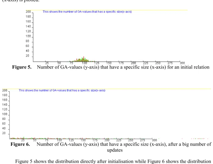
In a first version of the benchmark environment we implemented (3) and conducted experiments. When the nature of the updater was analysed some problems were identified. Figure 5

and Figure 6 show graphs in which the number of GA-values (y-axis) with a specific number of tuples (x-axis) is plotted.

Figure 5. Number of GA-values (y-axis) that have a specific size (x-axis) for an initial relation

Figure 6. Number of GA-values (y-axis) that have a specific size (x-axis), after a big number of

updates

Figure 5 shows the distribution directly after initialisation while Figure 6 shows the distribution after thousands of update transactions. The distributions are notably different. The biggest problem, however, is that the extreme values seem to move gradually as more updates are committed. In other words there may be no upper bound on the size of the biggest update. It is an undesirable property that the length of an experiment should have an impact on its outcome. As an example, if we double experiment time it does not imply that roughly the same situation is repeated twice. The latter half will have larger variations in update size.

Our final choice of update strategy is (4). As mentioned above it has a disadvantage in that changes are clustered. Comparisons with update model (3), however, did not show any notable differences in the results of experiments. This indicates that at least for the current DBMS this clustering has little impact.

6.3.2. The implemented solution (4)

Before running an experiment, the data generator fills the source relation by executing a number of insert transactions. The structure of a tuple (and consequently of a table) has no particular

• A View Attribute column: used to select which rows belong to the DW view; • A Guide Attribute column: directs the course of the update stream.

Apart from these fields, there are no constraints about the number and the nature of the rest of the attributes. At the same time the size of a row should be kept flexible in order to allow users to define the size of tuples for a specific experiment. Once defined, however, the size is fixed for the run. We have thus found it practical to define a fourth attribute governed by a parameter which dictates the size of a char type field. The result is that users have control over both the size and number of tuples in the source table.

The overall structure of the source relation is shown in Table 4.

Table 4. The Source relation Attribute Data type Description

PK Integer Primary key

VA Integer View attribute: used to define the DW view, if this attribute is 1 the tuple belongs to the view

GA Integer Guide attribute: used for set-oriented updates and deletes VSF char(size) Variable size field: used to enable different tuple-sizes.

Given such a structure, the data generator carries out its task by taking as input parameters the initial size of the table (number and size of tuples), the DW view selectivity and the update size. The initial number of tuples in the table is important. It dictates the range within which we pick the primary keys to insert in the table. In order to avoid any significant ordering or clustering, we set the range of possible primary key values to be significantly larger than the number of rows in the table. The view selectivity parameter is important to distributing the value of the ‘view attribute’ (VA). If the view selectivity is 0.1 then we randomly arrange 10% of the inserted rows to have VA set to one and therefore to belong to the DW view. No indexing is used on the VA field, which means recomputes will be more expensive.

The average number of tuples in each update transaction, L, is given by user settings. For each insertion we pick the size according to a normal distribution with expected value L (and a standard deviation which is user specified). The GA value can be any value which is not present in the relation.

If the table size is specified to be N tuples, the initial table is created by executing N/L insert transactions where the GA-value is picked sequentially from 0 to N/L-1. No indexing is used on the GA field4_.

Finally, tuple size is used in generating a random string of characters (a-z) to be inserted into the VSF of each row.

As soon as the execution of an experiment starts, we apply the stream of updates. Relevant parameters are the probability of having update against insert/delete to be performed and, once again, the update size. The probability parameter expresses the probability that the next update will be a true update, as opposed to an insert or a delete. Let for instance the probability of having an update be 0.6. This means that six times out of ten a true update will occur and four times out of ten an insert or a delete will occur. We decided to fix the probability of having an insert against a delete at 0.5. For our example, we will on average have two inserts and two deletes in every ten updates. Notice that the table may indefinitely increase (more inserts than deletes) or degenerate to the empty size (more deletes than inserts), if differently chosen. Thus, each time an update has to be performed, we decide which type of update will happen on the basis of the probability parameter. If an update or a delete are to be executed, the tuples to be affected are chosen by means of a where clause including the randomly selected existing GA value. In the case of an update, we replace the string in the VSF by a new one. For each tuple we permute a string by changing a character at a random position.

When an insert transaction is executed, we insert a number of tuples according to a normal distribution, all with the same (currently unused) GA-value. Update transactions will not change the number of tuples in a relation. When a GA-value is deleted, all tuples with that GA-value will be removed. This means that the size of the table will fluctuate around its original value as long as insert and delete transactions have the same probability.

6.4. Scheduling of updates

Up to now we have only discussed approaches to how to execute changes to a relation. We also need to address when to schedule transactions. A common statistical model is to assume updates to be Poisson distributed, which gives a good model of many real world phenomena, for example users independently modifying a database. It is, however, not possible to model all processes with a Poisson distribution. The cost-model of [Eng00] assumes that events are distributed evenly and that there is a fixed delay between events. This is not appropriate in a simulation. Firstly, it is not typical of any practical database scenario. Secondly, from a practical viewpoint, if we have several processes (update

and queries) which use fixed delays, the initialisation timing will potentially have a huge impact on experiment results and it may be very hard to detect worst case staleness values (in the cost-model this is not a problem as the worst-case situation can be derived analytically).

To avoid this problem in simulations we must use a distribution which has some variation around the expected value. An initial choice might be the Poisson distribution. However, this can have certain practical implications. In particular, because values generated by such a distribution are not bounded then experiments may be subjected to extreme periodicities. As explained in section 8, this may lead to simulation ‘overflows’. It is also questionable whether a Poisson distribution accurately represents the load on a source database, which will be subjected to regular update applications as well as casual user queries.

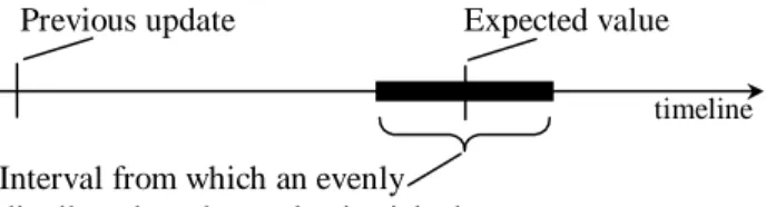
For both of these reasons it was decided to use a variation of even distribution, with events evenly distributed in an interval centred on an expected value. Figure 7 illustrates how delays are picked from this distribution.

timeline

Previous update Expected value

Interval from which an evenly distributed random value is picked

Figure 7. The distribution of the delay between updates

In the figure the interval is 40% of the expected value. When running a simulation, users specify an average delay between updates and a variation interval as a percentage of this delay. By specifying the variation width to 0%, the distribution will be fully regular and deterministic.

We have chosen to provide the option to run experiments using different distributions (including Poisson). This can be used to explore maintenance under different update and query assumptions. In particular, in order to ensure that this choice did not lead to highly particular results, a number of experiments have been run with both Poisson and the even distribution with variation. Figure 8 illustrates the difference between even distribution, with and without variations, and Poisson distribution. The expected value is the same for all distributions and the variation is 40%.

Figure 8. Even distribution (with and without variations) against Poisson distribution

It is interesting to note that the two even distributions have a similar pattern while Poisson is notably different. In the experiments where these distributions were compared, there is an indication

that the impact on performance is less significant. A full investigation is, however, outside the scope of this paper and is left for future work.

6.4.1. Enforcing distributions

If the time to execute an update is not negligible, then it is important that the delay between updates is computed from the start of one update to the start of the next. For example, a computed value should not be used as the delay from when one update is finished until the next is started. If this is done we will have fewer updates per time unit than expected.

In our model we record the time an update is started and compute the (absolute) time when the next update should start. When the first update is completed we compute the required delay. If the remaining time is negative this implies that the update took longer than the delay between updates. This is an undesirable situation and we record it as an overflow. If an experiment has many overflows it indicates that the system is saturated and parameters need to be adjusted.

7. Implementation

To be able to observe and measure maintenance policies in a controlled fashion, we have implemented a benchmark environment which is run on dedicated hardware. Standard software is used as much as possible. In order to realise the variety of functionality addressed by the cost-model, we have also developed software components to handle maintenance. We have moreover developed simulation entities for the generation of updates and queries, and to facilitate measurement. The resulting environment makes it possible to specify a set of experiments which will be conducted and reported in a concise format. A large number of system parameters may conveniently be specified and altered.

The goals presented in section five have guided this work and the development has been iterative. This means that experiments have been conducted continuously to verify that goals have been met. Details of the implementation, including a class diagram, appear as an appendix. In this section we highlight some important design decisions.

7.1. System description

The system has been developed as a distributed application, with an Interbase 6.0 source database running under Solaris 8 on a 360 MHz Sun Ultra Sparc IIi with 384 Mbytes RAM, 0.2 Mbyte cache and an IDE disk. The client DW was run under Solaris 7 on a 167 MHz Sun Ultra Sparc I with 256 Mbytes RAM and 0.5 Mbyte cache and a SCSI disk. The machines are connected via a 10Mbit hub. During experiments the hub has no other computers connected to it, neither is it connected to any

active. Swap is disabled on both machines, which means that experiments will halt if main-memory is too low. In this way we automatically avoid thrashing.

All software is developed in Java and run on JVM 1.3.0 from Sun. Communication between different processes is handled via Java RMI. All security restrictions have been disabled which means that remote invocations can initiate any activity on the local machine. This is useful for locating the wrapper and performing initialisation. In a real environment this is an obvious security threat, but as our experiments are run on an isolated network, security can be ignored.

Database access is handled with JDBC using the native Interbase Interclient 1.6 driver.

7.2. Overview of the environment

To conduct an experiment the user has to specify configuration parameters, and create and populate an initial database which can be used for a set of experiments. This is done by using a GUI-based tool, which is described in appendix A. Interbase will typically store a database in a file located in the local file-area of the database server. It is possible to duplicate a database by copying its file. This is done before each experiment in order to have an identical database start image for each experiment in the set.

To conduct experiments, a script has to be started on the source machine. This will create and initiate an updater and a “source server” which will await requests from the director. The server-side programs do not require any configuration – they receive a configuration object through a RMI message from the director. For each new experiment the source server and updater will be automatically restarted to avoid potential dependencies on previous experiments (for example related to memory management).

The director, warehouse, and querier are started from the client machine. This is done through a script which can contain any number of experiments that will be executed sequentially. For each experiment a configuration is specified. This is read by the director, who will initiate all other components. This includes propagating a configuration object and sending requests to start operation. The random number generators are initialised with a seed, which is specified in the configuration. The source server will be asked to copy the initial database file to a new location.

If the wrapper is to be located at the server machine, the source server will create a wrapper object and give the integrator a reference to it. If the wrapper is to be located in the warehouse, the director will create it.

The result of an experiment is written to a file which contains parameter settings, measures, errors and other information. The name of the file will contain a number which orders logs according to start time. When all experiments have been conducted, logs can be automatically processed and summarized into a single table.

7.3. Modelling source properties

Interbase has solid trigger functionality which we utilise to provide DAW. This is done by defining triggers which insert changes to the source table into an auxiliary table, which we also define. We do not disable triggers even when DAW is not utilised. The reason for this is to exclude the overhead associated with the trigger implementation of true DAW, as discussed in section six5_.

CHAC is more difficult to achieve. Interbase has a mechanism for event notifications in embedded SQL where threads can wait for events to be signalled from, for example, triggers. This mechanism is not available through JDBC, however. In addition it is not possible to generate events on transaction commit, which is crucial for consistent maintenance. What we do in the benchmark system is to let the source updater notify the wrapper after each commit. This is a way to emulate source capabilities which a real system does not have. We claim that this is acceptable for our purposes. We carefully design the message passing to avoid blocking and we monitor the overhead it introduces in terms of RMI communication.

To emulate CHAW, the wrapper is given the latest update sequence number from the source updater. This can be seen as a logical timer which increases with each update. The wrapper records the time of the modification used in the last message to the integrator (the sequence number). It is possible to decide whether the source has been updated by comparing the current number with the recorded value.

Interbase is obviously view-aware for views expressed in SQL.

7.4. Wrapper operation

The wrapper will make use of a source capability if the configuration specifies that the capability is present. Otherwise it will adjust its operation accordingly. If DAW is absent the wrapper will keep a snapshot of the view and, when deltas are required, will retrieve a new snapshot from the source and perform a diff. The diff operation uses a sort-merge algorithm to detect changes. The old snapshot is finally replaced with the new, sorted snapshot.

If the source is change aware, the wrapper can ignore maintenance if no changes have been committed since last maintenance. If it is not CHAW, or if changes have occurred, maintenance has to be conducted.

CHAC does not affect wrapper operation since it is required for immediate policies and if CHAC is not present those policies can simply not be used. It is the responsibility of the person who configures an experiment not to use immediate policies if CHAC is not present.

If the source is configured not to be view aware the wrapper will retrieve the whole source and compute the view by iterating through the result-set. Currently this is only done for recompute policies. It can be meaningful to explore incremental policies with neither DAW nor view awareness.

7.5. Processes and threads

When an experiment is executed the source updater will run in one Unix process on the source host (server). The director and warehouse will run in one Unix process on the DW host (client). Depending on localisation the wrapper will run in an independent process on the server or as part of the director and warehouse process on the client. All these processes will execute as Java programs with default priority. In addition there will be a RMI registry and an Interbase server both running on the server.

The source updater process has one thread which is active when changes are performed. It sleeps between changes. The time spent in execution is recorded in the log of an experiment.

The director and warehouse process has one thread for the querier which is similar to the updater. The director and warehouse have no threads. The wrapper, which may be located in the warehouse, has its own thread. Both the client and the server have a ClassFileServer. This is a thread which waits for requests for class-files. It is needed for RMI-communication and is active only during initialisation. The server has a further thread if the wrapper is located in the server.

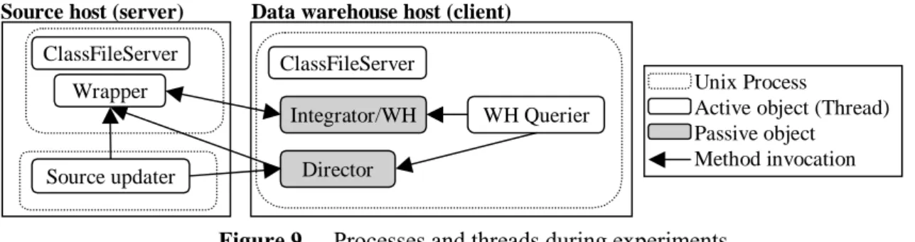
To summarise, there are three processes and five threads during experiments6_{. Figure 9} illustrates this and shows runtime interactions.

Source host (server) Data warehouse host (client)

ClassFileServer _{ClassFileServer} Director Integrator/WH WH Querier Wrapper Source updater Unix Process

Active object (Thread) Passive object

Method invocation

Figure 9. Processes and threads during experiments

As can be seen from the figure, the wrapper, integrator and director can be accessed by more than one thread. These classes have been carefully designed to ensure safety and liveliness properties.

6 _{Actually the ClassFileServer forks threads for each requested file, but as mentioned above, it is not active}

For a benchmark it is very important that independent processes are not accidentally synchronized by method invocations related to the instrumentation.

The querier and updater threads call the director object but these calls do not manipulate any shared data and there is no need to use a monitor. The integrator may receive calls from querier and wrapper but the queries only require computations when on-demand is selected. In those cases the wrapper will only send messages to the integrator as a response to a request. This gives synchronous invocations. The wrapper is the most complex object in terms of thread synchronisation. The calls from the updater are used to initiate immediate maintenance, but we do not want these calls to be blocked if the wrapper is active. To handle this we let the wrapper thread wait for notifications and we use a counter to keep track of the number of changes reported. If the wrapper thread is active when a notification is sent, it will still be able to detect it. The same mechanism is used for on-demand policies where the notification comes from the integrator. Periodic policies are simpler as they are initiated within the object itself.

Finally, for threads which should generate events according to some distribution, we use the algorithm shown in Figure 10 to enforce conformance to the distribution.

startT=getCurrentTime(); while(alive) begin delay=getDelay(); startT=startT+delay; doTask(); sleepT=startT-getCurrentTime(); if(sleepT<0) begin reportError(“Overflow”); startT=getCurrentTime(); end else sleep(sleepT); end;

Figure 10. Algorithm used to conform to a distribution.

In the pseudo-code we make a function call getDelay() to get the computed delay according to the distribution selected. For periodic policies this is the delay specified in the configuration. The function getCurrenTime() returns the current value on the system clock. The procedure doTask() performs the task we are scheduling, e.g. performs an update.

7.6. Metrics

7.6.1. Integrated cost

The integrated cost is the sum of processing conducted in the warehouse and source together with the communication delay. By carefully designing wrapper and warehouse interaction, we may

and the time waiting for communication and for the integrator to insert changes. To achieve this we let the integrator block the call from the wrapper until maintenance has been conducted and a Boolean value is returned. The way to measure the integrated cost is unaffected by the localization of the wrapper. Obviously, there is no way to break down computed IC into individual components.

During runtime, the aggregated integrated cost for each query is stored in an array in the integrator. When a query has been reported (from the querier), the director retrieves the current aggregated IC from the wrapper. When an experiment has finished, these values are used to compute additional measures such as the average IC per query, and the variation of IC when the experiment time is split into ten periods.

It should be noted that measurement might be affected by the scheduling of threads. That is, if several threads are active we will have an increase in IC which is not due to maintenance activity. It is impossible for us to completely control this. If a JDBC call is delayed, there is no way to derive the actual delay from the delay caused by context switching in the source computer. What we can do however is to monitor the activity of other threads within the benchmarking environment. If the total execution time in other threads is low, the measured IC will be representative. By contrast, if the source machine is saturated with frequent updates, the measured IC will most probably contain “noise”. For these reasons we believe it is advisable to run experiments with a non-saturated configuration. However, the importance of this issue should not be over-stated, as it may not have any impact on the outcome of experiments. We are interested in comparing the relative difference between policies, and not absolute values.

7.6.2. Staleness and response time

Staleness and response time are computed as described in section 5. To reduce the probe effect the director creates arrays before the experiment is started to contain reported values. The sizes of these arrays are chosen to be sufficiently large to minimise the risk of overflow. As we use random distributions it may happen that the source is updated, for example, twice as many times as expected. In theory, any chosen fixed array size may lead to overflow. We take a pragmatic approach and choose a size which has a very small risk of overflow7_{. If an overflow occurs this will be reported in the log} and the results from that experiment will not be used.

7.6.3. Additional information collected

As described in 5.5.4, in addition to the metrics which corresponds to the cost-model, each experiment records information which is useful for verifying the correct behaviour of the system and

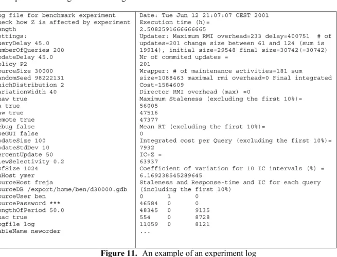
that the experiment has been successful. All information collected is saved in an experiment log. An example of such a log is shown in Figure 11.

Log file for benchmark experiment check how Z is affected by experiment length Settings: queryDelay 45.0 numberOfQueries 200 updateDelay 45.0 policy P2 sourceSize 30000 randomSeed 98222131 whichDistribution 2 variationWidth 40 chaw true va true daw true remote true debug false useGUI false updateSize 100 updateStdDev 10 percentUpdate 50 viewSelectivity 0.2 vsfSize 1024 whHost ymer sourceHost freja sourceDB /export/home/ben/d30000.gdb sourceUser ben sourcePassword *** lengthOfPeriod 50.0 chac true logfile log tableName neworder

Date: Tue Jun 12 21:07:07 CEST 2001 Execution time (h)=

2.5082591666666665

Updater: Maximum RMI overhead=233 delay=400751 # of updates=201 change size between 61 and 124 (sum is 19914), initial size=29548 final size=30742(=30742) Nr of commited updates =

201

Wrapper: # of maintenance activities=181 sum

size=1088463 maximal rmi overhead=0 Final integrated Cost=1584609

Director RMI overhead (max) =0

Maximum Staleness (excluding the first 10%)= 56005

47516 47377

Mean RT (excluding the first 10%)= 0

Integrated cost per Query (excluding the first 10%)= 7932

IC+Z = 63937

Coefficient of variation for 10 IC intervals (%) = 6.169238545289645

Staleness and Response-time and IC for each query (including the first 10%)

0 1 0 46584 0 0 48345 0 9135 554 0 8728 11059 0 8121 ...

Figure 11. An example of an experiment log

The second line in the log is a description of the experiment which the user can specify to remember the purpose of a set of experiments. The rest of the left hand column in the figure reports the settings used. The right hand column contains all the information collected. The first line gives the date when the experiment was completed and is followed by the total execution time. The following five lines contain various pieces of information collected by the source updater. For the log shown, we can conclude that the maximal delay to communicate with wrapper and director was 233 ms. This means that the update time recorded by the director, and used in staleness computation, has an error bound of 233 ms. We see that the total time spent in the updater doing updates was less than 7 minutes (400 s). We also get details of the number of updates, the size of updates and the size of the source relation. This is followed by similar information from the wrapper and director.

Finally, the log presents computed measures. In computing these measures we ignore the first 10% of the queries, which are considered to relate to the warm-up time. If the warm-up time is to be analysed or varied, values for all individual queries appear at the end of the log (in the figure we only present values for five queries). This means that additional measures, with different length of warm-up

If there have been any errors during an experiment, these are also listed in the log.

7.7. Post-processing

An experiment consists of several benchmark tests, and analysing several files each with a large number of measures is an error-prone task. Therefore we have developed a filter which takes any number of logs and summarises interesting information into a single file. This can then be processed, for example using a spread-sheet program. Individual queries are excluded; only summarised measures are shown. A measure or setting is included if at least two experiments have different values for it. In other words, properties which are not varied are not included in the summary file. These settings can, however, be found in any of the log-files on which the summary is based. Figure 12 shows an example of such a summary translated into a spreadsheet, with a plot added to aid in visualising the results.

Figure 12. An example of summary results from several experiments

8. Experiments

As described in the previous section, our benchmark environment makes it possible to run a set of experiments, process the results and then analyse them. In this section we present results from a number of experiments that have been conducted. First we present experiments conducted to verify the correctness of the implemented system; what we call ‘sanity checks’. Then we present a number of experiments which were designed to allow comparison with the cost-model.

All experiments described in this section have been conducted in an isolated environment. During analysis we inspected the logs to verify that no errors or unexpected events occurred during execution.

8.1. Sanity checks and verification of the environment

8.1.1. Updater

A number of basic sanity checks were initially conducted on the system. Our first check was of the updater, and in particular confirmed that the average size of the generated database was maintained