Machine Learning assisted system for the resource-constrained atrial fibrillation detection from short single-lead ECG signals

(1)

Machine Learning assisted system for the

resource-constrained atrial fibrillation

detection from short single-lead ECG signals

Anara Abdukalikova

Computer Science and Engineering, master's level (120 credits) 2018

Luleå University of Technology

(2)

This thesis is prepared as a part of an European Erasmus Mundus program PERCCOM - Pervasive Computing & COMmunications for sustainable development.

This thesis has been accepted by partner institutions of the consortium (cf. UDL-DAJ, n°1524, 2012 PERCCOM agreement).

Successful defense of this thesis is obligatory for graduation with the following national diplomas:

• Master in Complex Systems Engineering (University of Lorraine)

• Master of Science in Technology (Lappeenranta University of Technology)

• Master of Science – Major: Computer Science and Engineering, Specialisation: Pervasive Computing and Communications for Sustainable Development (Luleå University of Technology)

(3)

ABSTRACT

Luleå University of Technology

Department of Computer Science, Electrical and Space Engineering Erasmus Mundus PERCCOM Master Program

Anara Abdukalikova

Machine Learning assisted system for the resource-constrained atrial fibrillation detection from short single-lead ECG signals

Master’s Thesis

64 pages, 21 figures, 8 tables, 3 appendices

Examiners: Professor Eric Rondeau (University of Lorraine)

Professor Jari Porras (Lappeenranta University of Technology) Associate Professor Karl Andersson (Luleå University of Technology)

Keywords: E-Health, Atrial Fibrillation detection, ECG, Machine Learning, Recursive Feature Elimination, Sustainability

An integration of ICT advances into a conventional healthcare system is spreading extensively nowadays. This trend is known as Electronic health or E-Health. E-Health solutions help to achieve the sustainability goal of increasing the expected lifetime while improving the quality of life by providing a constant healthcare monitoring. Cardiovascular diseases are one of the main killers yearly causing approximately 17.7 million deaths worldwide. The focus of this work is on studying the detection of one of the cardiovascular diseases – Atrial Fibrillation (AF) arrhythmia. This type of arrhythmia has a severe influence on the heart health conditions and could cause congestive heart failure (CHF), stroke, and even increase the risk of death. Therefore, it is important to detect AF as early as possible. In this thesis we focused on studying various machine learning techniques for AF detection using only short single lead Electrocardiography recordings. A web-based solution was built as a final prototype, which first simulates the reception of a recorded signal, conducts the

(4)

preprocessing, makes a prediction of the AF presence, and visualizes the result. For the AF detection the relatively high accuracy score was achieved comparable to the one of the state-of-the-art. The work was based on the investigation of the proposed architectures and the usage of the database of signals from the 2017 PhysioNet/CinC Challenge. However, an additional constraint was introduced to the original problem formulation, since the idea of a future deployment on the resource-limited devices places the restrictions on the complexity of the computations being performed for achieving the prediction. Therefore, this constraint was considered during the development phase of the project.

(5)

ACKNOWLEDGEMENTS

This thesis was conducted as a part of the Erasmus Mundus Master programme in Pervasive Computing and Communication for Sustainable Development (PERCCOM) funded by the European Union.

I would like to express my sincere gratitude and great appreciation to my supervisors Doctor Denis Kleyko and Professor Evgeny Osipov, who believed in me and constantly supported throughout the whole work process. This thesis would not have been possible without their continuous guidance and valuable feedback, which always encouraged me. Thank you, Denis, for always being there and giving me advices, which helped to conduct this thesis.

I would also like to thank Professor Eric Rondeau, Professor Karl Andersson, Professor Jari Porras and all PERCCOM staff for their academic support during the whole PERCCOM time. I am grateful to PERCCOM Consortium for giving me a chance to be a part of this amazing two-year journey, which brought me many unforgettable memories shared with the friends I was lucky to meet.

A special thank to my family, who never stopped believing in me throughout my entire life. I am extremely grateful to have the most understanding parents and the greatest sister, who always supported me in all my beginnings.

(6)

6

LIST OF SYMBOLS AND ABBREVIATIONS

AF Atrial Fibrillation

ANN Artificial Neural Network

ApEn Approximate Entropy

AWS Amazon Web Services

CD Correlation Dimension

CHF Congestive Heart Failure CNN Convolutional Neural Network

DNN Deep Neural Network

EC2 Elastic Compute Cloud

ECG Electrocardiography

EMG Electromyographic

HF High Frequency HRV Heart Rate Variability

HTML Hyper Text M Language

kNN k Nearest Neighbour

LDA Linear Discriminant Analysis

LF Low Frequency

LLE Largest Lyapunov Exponent

LSTM Long Short Term Memory

LTV Long Term Variability

MF Medium Frequency

MVC Model View Controller

RFE Recursive Feature Elimination

RMSSD Root Mean Square Successive Difference of intervals RNN Recurrent Neural Network

RQA Recurrence Quantification Analysis

SD Standard Deviation

SDANN Standard Deviation of mean of NN intervals in 5 min SDNN Standard Deviation of the NN intervals

(9)

9

SENN Standard Error of the mean of NN intervals SQI Signal Quality Indices

SQL Structured Query Language STFT Short Time Fourier Transform STV Short Term Variability

SVM Support Vector Machine

WHO World Health Organization XGBoost eXtreme Gradient Boosting

(10)

10

1 INTRODUCTION

According to Principle I of the Rio Declaration on Environment and Development, which state [1]: “Human beings are at the centre of concerns for sustainable development. They are entitled to a healthy and productive life in harmony with nature”, world sustainability goals cannot be fully achieved while there is still high mortality rate due to widely spread debilitating illnesses, such as skeletal, cardiovascular, lung, neuromuscular diseases and some others. In addition, the issue of increasing aging population also necessitates improvement and development of technologies for constant health monitoring, since most of the diseases, especially cardiovascular ones, increase in accordance with aging and requires regular checks. Therefore, in order to achieve sustainability in the world, it is crucial not only to provide environmentally good-living conditions, but also to keep global population health as one of the main priorities. Wellbeing of world's nation is at utmost importance and provision with modern tools for health monitoring contributes to strengthening preventative healthcare system, as well as enhancing early diagnostics capabilities. Thus, the sustainability goal of increasing life expectancy and improving quality of life may be achieved. The process towards these objectives includes integration of Information and Communication Technologies advances into a conventional healthcare system which relates to E-Health area. The idea of “doctor in your pocket” will improve the whole chain of healthcare provision [2]. Patients will be able to regularly monitor and control their health conditions, eliminating the time spent in hospital corridors waiting for the medical check-up.

E-Health solutions are aimed at empowering people to better manage their health and lifestyle by equipping them with tools for enhanced health monitoring and ability to cope with associated conditions. Currently European Commission and many EU countries put their priorities on making E-Health records systems, the deployment of telemedicine services and patient safety more interoperable for enhancing care, mobility and safety of patients [3]. If E-Health tools were available for the majority of people and were easy in use, they would significantly contribute to improvements in medical care provision on the whole.

(11)

11

1.1 Motivation

Nowadays, people are induced to keep up with the high pace of life so that in most cases they have to sacrifice their health care, as well as with the aging population it would be harder to get a routine visit to a doctor. Unregulated diet, lack of physical activity, environmental factors and many other habits caused by the lack of time significantly affect health conditions, specially causing heart-related problems. In order to provide timely medical help, it is crucial to detect cardiovascular problems at an early stage. Therefore, the development of handy E-Health tools may contribute to improvements in early detection and prevention of cardiovascular diseases.

According to the statistical data provided by World Health Organization (WHO) [4] approximately 17.7 million people die annually around the globe from cardiovascular diseases, which is 31 % of the total number of deaths worldwide. This number is expected to grow up to 23.3 million deaths per year by 2030, which shows how rapidly this problem is spreading. This is giving more importance on researching cardiac health and developing more advanced preventative tools. Thus, it will contribute to the improvement of the cardiovascular diagnosis technologies, particularly enhances in digital electrocardiography (ECG) analysis. And as stated earlier E-Health solutions will have positive impact on the whole healthcare system [2]. The focus of this thesis is laying in the researching one of the possible causes of heart-related diseases, i.e. detection of atrial fibrillation.

Atrial fibrillation (AF) is a supraventricular tachyarrhythmia which is represented by inconstant atrial activation and therefore dysregulations of atrial contraction. Atrial fibrillation is considered to be the most common form of heart arrhythmia and has 1-2 % of occurrence among the general population with the increasing number due to age. Over 6 million Europeans have this type of arrhythmia and it is estimated that the number will increase within next 50 years twice [4]. According to Framingham Heart study [5], risk of AF was observed in 26 % of men and 23 % of women at the age of 40 in Europe. Moreover, the incidence of AF in past two decades increased for 13 % and is expected to grow substantially. Atrial fibrillation is considered to cause the morbidity and mortality, as well as the increment in risks for death, congestive heart failure (CHF), and embolic phenomena such as stroke. AF increases the possibility of stroke around 5-fold and it is proved that one

(12)

12

of five strokes refers to this type of arrhythmia. It was studied that most of the ischaemic stokes in association with AF are fatal, and patients who survived are mostly disabled for a long time and have high chance of the repetitive stroke [4]. AF related diseases significantly influence on quality of life and therefore its early detection plays an important role in sustainable development of the global population.

AF may remain protractedly undiagnosed and this is called “silent AF”. Due to this factor most of the patients are often unaware of its presence, therefore early recognition of AF is crucial and requires reliable tools for its detection. The development of these tools may help to reduce the severe consequences caused by AF as well as to prevent the progression from early and easy treated stages to utterly deteriorated ones. Additionally, AF-related costs for care have 1.5-fold increment which is related to the double number of death risk from the strokes caused by AF, thus early diagnosis of AF may reduce costs related to its treatment [4].

All the above-mentioned statistics shows that atrial fibrillation presence may utterly affect human health and increase the risk of being disabled after having a stroke. Therefore, timely detection of AF may eliminate related serious consequences.

1.2 Problem definition

Cardiovascular diseases are known to be the world's most widespread killer, early detection of its causes is extremely important to ease the subsequent treatment and help to take corresponding measures on early stages. High potential of Atrial Fibrillation to cause the long-term disability of patients makes its early detection crucial for preventing life-threatening consequences. The work on solving this problem has been done before and different detection techniques were used. However, most of the studies concentrated on using machine learning techniques. Since it is rather hard to come up with a static rule-based algorithm for AF detection, using machine learning has high potential to solve this type of problem. Although most of the previous studies showed quite high and promising results, they had a number of limitations. Small sized datasets were presented by carefully selected signals of only two types: AF and normal. Moreover, previous studies approaches were trained and adapted only to the signals having the long duration and being recorded from

(13)

13

several leads. Thus, this thesis addresses the problem of atrial fibrillation detection from short single-lead Electrocardiography (ECG) recordings by using machine learning techniques. In this thesis we investigated the proposed architectures and used the database of signals from the 2017 PhysioNet/CinC Challenge. The dataset in this challenge was bigger and was presented by four different types of short single-lead ECG recordings. However, the idea of future deployment on the resource-limited devices places the restrictions on the complexity of the computations. Practical limitations require that the diagnostic can be done outside a hospital using inexpensive equipment and without an involvement of medical staff. Also, the time required to make a test should be short.

1.3 Goals and delimitations

The goal of this master thesis was to develop, implement and validate an accurate, efficient and sustainable solution for Atrial Fibrillation detection from the short-lead ECG signals (between 30 and 60 s) which should have relatively high accuracy in predictions. The AF detection should be realized in an accurate and fast manner with the future potential to be used in real-time monitoring of abnormalities in ECG signals. The output of signals classification had to provide one of four classes: normal sinus rhythm (Normal), atrial fibrillation (AF), an alternative rhythm (Other), or too noisy to be classified (Noise). Since most of the previous researches did not provide classification for more than two classes, it makes the problem of this thesis more sophisticated.

In this thesis, the final deliverable of the project should also include an interactive user-friendly web application prototype. It should allow users to upload their own recorded ECG signals and by means of the machine learning algorithms get a prediction on AF presence or absence.

Delimitations: this study mainly concentrated on the development of the working core for

AF detection and did not include designing the whole system, which would include the real-time signal reception from sensors and the deployment on a handy device.

(14)

14

1.4 Research methodology

In every research it is highly important to correctly choose a research methodology, since the main work flow is realized according to it. The achieved goals and results of the project are directly related to the properly chosen methodology.

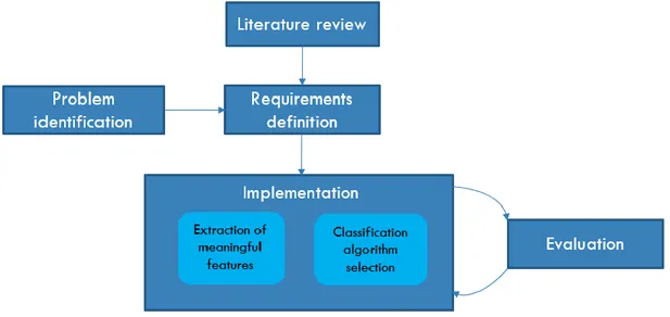
This thesis was conducted in accordance with the methodology illustrated in the Figure 1.1.

Figure 1.1: Thesis methodology.

The first stage of the work process included critical literature review, problem identification and research gaps definition. Work process and system requirements definition were the next step followed by the practical part of the research. It comprised an iterative process of an implementation and a corresponding evaluation of the results. Implementation included two main parts: feature extraction and selection of an appropriate machine learning algorithm for classification.

1.5 Structure of the thesis

This section provides an information about the thesis structure with a brief description of each chapter.

 The INTRODUCTION gives an overview and understanding of the necessity of studying the detection of heart related diseases, covers the sustainability of the

(15)

15

problem as well as the implemented research methodology. The particular problem of AF detection is described in detail.

 The RELATED WORK chapter presents the review of the relevant studies made in this area. It includes previous studies related to the binary classification of AF, as well as the analysis of the approaches for multiclass classification from the 2017 Physionet/CinC challenge.

 The AF DETECTION IMPLEMENTATION chapter includes the detailed description of the signal pre-processing, the feature extraction and the implemented machine learning algorithms stages.

 The EVALUATION AND RESULTS chapter provides the evaluation of various feature sets training and their comparison. The proposed computations reduction solution is also described in this chapter.

 The WEB APPLICATION PROTOTYPE chapter describes the development and the process flow of the web application built for the visualization purposes of the proposed solution.

 The CONCLUSION AND FUTURE WORK chapter gives a brief summary of the work. In addition to that, future development and possible improvements are also discussed.

(16)

16

2 RELATED WORK

In this chapter we look at the nature of ECG signals and investigate the researches done in solving AF detection problem. All proposed approaches in the previous studies was divided into two subsections: the ones made by various individual researches and the others made in the framework of PhysioNet/Computing in Cardiology Challenge 2017. The discussion of the proposed approaches is also provided, followed by their comparison presented by the tables.

2.1 ECG signals

The ECG [6] is a technique used to record the cardiac electrical activity over a period of time, which is presented by the time-voltage chart of the heartbeat. The ECG is the main tool for diagnostics of various cardiac conditions and diseases. It corresponds to cardiac electrical activation (depolarization) and relaxation (repolarisation) [7] and represented by several main wave complexes (P, Q, R, S, T, U) as shown on the Figure 2.1.

Figure 2.1: ECG main wave complexes [7].

P wave of the signal corresponds to the atrial depolarization related to the upper chamber of the heart [7]. The transition of an electrical impulse from the upper chamber of the heart to

(17)

17

the lower one is depicted as PR interval. The depolarization of the lower chamber of the heart (ventricle) corresponds to QRS interval. The repolarization of the ventricle is represented by the ST segment and T wave complex.

2.2 AF detection from ECG signals

The problem of AF detection has been investigated previously and most of the implemented methods showed rather good and promising results, however, all of the previous studies [8]– [12] had a number of limitations in their applicability. For instance, the classification was conducted only between two classes: normal and AF signals, predominant part of which was noise-free and was thoroughly picked out. Moreover, in most of the cases the dataset was represented by a small number of samples. Even though most of the solutions showed high sensitivity in predictions, the future possible accuracy of those results is questionable.

Every heart arrhythmia can be identified by its own specific features. Every ECG signal is presented by basic waves: P, Q, R, S, T and U, and cardiovascular anomalies detection is based on the analysis of these waves nature. There are several morphological features particular to AF, such as absence of P wave, the presence of fluctuating waves instead of P waves, and irregularity in intervals between R peaks (RR intervals) [8]. However, it is hard to detect AF according to P wave absence factor, since its amplitude is rather small and it could deteriorate detection in the presence of noise. Thus, many studies concentrate on learning the heart rate irregularity, which is presented by inconsistent intervals between R peaks. This is related to one of the main AF characteristics, when the atrium (the upper chamber of the heart) quivers instead of beating regularly, causing disturbances in the blood flow. So, in case of clot break, it can get stuck in the artery, thus leading to a stroke.

Methods based on RR intervals are proposed in many studies, since it is easier to extract R peaks from ECG signals due to its comparably high amplitude. In [13] authors received high sensitivity and specificity of 93.2 % and 96.7 % respectively, using the comparison between standard density histograms and a test density histogram by the Kolmogorov-Smirnov test of RR and delta RR intervals. In this work the dataset was comprised of small amount of samples with the duration varying between several hours. In other researches, such as [9], [10] and [11], authors were proposing AF detection methods based on Poincare plot features.

(18)

18

However, the features extracted from these plots varied in each of these studies. All of these works' results showed high specificity and sensitivity scores, but the datasets were still remaining small. Additionally together or separately from Poincare plot features, some authors were using features received from heart rate variability (HRV) analysis, which included time domain, frequency domain and non-linear features [14]. For instance, in [12] authors extracted only time domain and non-linear features and after classification stage they received 99.07 % sensitivity.

The procedure in all of these studies mostly included three steps: pre-processing of data, feature extraction and classification. On each of the stages different authors used various techniques.

2.2.1 Pre-processing of signals

Every analysis-based approach of ECG signals starts from initial signal processing techniques, which provides filtered, noise-free results. An accurate pre-processing has a significant influence on the further feature extraction and classification stages. Since most of ECG signals are obtained by placing electrodes on the human body, it leads to their contamination with noise. It can be presented by baseline wander, power-line interference, electromyographic (EMG) noise, electrode motion artefacts and some other noises [15]. The solution for elimination of interfering noises in signals is the implementation of various filter types. In [9] authors filtered ECG signals using two Butterworth filters: 4th order high-pass filter at 1 Hz for elimination of baseline wandering and a 8th order low-pass filter at 40 Hz for line interference and higher frequency noise components removal. Authors in [8] used sgolay filtering for removing baseline wander presented in segments, obtained from dividing signals into desired length. There was also presented another way to get rid of undesirable noisy parts in [12], which comprised of 5-15 Hz bandpass filter usage. It was aimed at removing 50 Hz power line interference, EMG noises and the baseline wandering. The next step in pre-processing of ECG signals for further analysis includes the detection of QRS complexes. This stage can be also presented by different techniques, such as Pan-Thomkins algorithm used in [12] and [14], algorithm developed by Christov [16] implemented by authors in [9] and wavelet method proposed in [17] and used by authors in [10].

(19)

19

2.2.2 Feature extraction methods

After obtaining QRS complexes, extraction of meaningful features plays an important role in further classification process and, therefore, highly influences on the final accuracy score. Many studies differed not only in the pre-processing techniques, but also in the features they were using in their works. The feature extraction process varied: some researchers were extracting features from Poincare plots as authors in [9], [10] and [11] did, others were concentrated on receiving more detailed information about signals by extracting HRV features [12]. Moreover, the combination of both was also used in [18].

Poincare plot is a graphical two-dimensional representation tool capable of displaying dynamic properties of a system from time series [19] into a phase space. Every point on this plot is represented by the values of a pair of successive elements of time series [20]. In case of ECG signals, the pairs of successive RR intervals are taken for visualization, i.e. the current RR interval is plotted as a function of the previous one. The visualization part in all the studies stayed the same, however the features extracted from these plots varied. So for instance in [10] authors extracted the number of clusters, mean stepping increment of inter-beat intervals, and dispersion of the points around a diagonal line in the plot, in [11] two generalized linear dependence coefficients and two root mean square errors for two and five consecutive heart beats cases were proposed, in [18] two types of standard deviation and the ratio between them were used.

For some cases in addition to Poincare plot feature extraction method, HRV analysis provided another set of significant features. Variations in the beat-to-beat timing of the heart represent the heart rate variability [20]. Since HRV signal has both linear and non-linear characteristics, its analysis includes both methods. Linear methods comprise of time domain and frequency domain analyses of the episodes, which can provide vast number of features. Non-linear analysis is able to describe the processes generated by biological systems in a more effective way [21] and includes the following techniques: Recurrence plots, Sample entropy (SampEn), Hurst Exponant (H), Fractal dimension, Approximate Entropy, Largest Lyapunov Exponent, Detrended Fluctuation analysis, and Correlation Dimension analysis [14]. In [12] authors used various features both from linear and non-linear analyses, however in [18] they limited number of features only to frequency domain and some non-linear features.

(20)

20

2.2.3 Classification algorithms

There are various approaches to detect atrial fibrillation based on the extracted set of features. For this purpose, different machine learning techniques were implemented, such as Support Vector Machine (SVM), Artificial Neural Network (ANN), Naive Bayesian classifier, k nearest neighbor (kNN) and some others. Many studies gave their preferences to SVM and ANN as the main AF detection classification tool.

Support Vector Machine is a supervised learning algorithm, which may be applicable to both classification and regression problems. By means of non-linear function SVM maps data points to a high-dimensional space, therefore making non-linearly separable data set linearly separable [22]. SVM aims at finding the best separating hyperplane (the plane with maximum margins) in two classes classification problem within the feature space by identifying the most representative training cases placed at the edge of the class [23], which are called support vectors. Even though SVM were initially elaborated for two-class problems, it may be applicable to multi class classification as well. This can be achieved by using one of the two approaches: either ``one against all'' or ``one against one'' methods, where classifiers are applied on either each class against all others or on each pair of classes respectively [23]. Training this type of classifier in [18], [11] and [8] showed high sensitivity and specificity scores (over 90 % in both cases).

Artificial Neural Network is a biologically inspired machine learning algorithm, which was designed based on nervous system of human brain [14]. It consists of input, output and hidden interconnected layers, which are comprised of connected nodes called artificial neurons. Every layer has predefined number of nodes, where the input neurons are equal to the number of features and the output ones depend on the number of classes. As for the hidden layer the number of nodes are specified by the user before the training and is based on the desirable performance of the classifier. During the training process of ANN the best weights for each nodes on every layer are received and used on the later testing phase for the classification [24]. Using this algorithm authors in [25] achieved high results with approximately 96 % accuracy.

(21)

21

The short comparison of the some of the above-mentioned studies is shown in the table below with some remarks taken regarding proposed methods.

Table 2.1: Comparison of various proposed approaches for AF detection Authors Preprocessing techniques Extracted features Classifiers Remarks Padmavathi K., Ramakr- ishna K. Sri Resampling at 128 Hz, segmentation of signal, sgolay filtering for noise

removal Autoregressive coefficients SVM, kNN The presented dataset was small (280 signals) Tuboly G., Kozmann G. Two Butterworth filters (4th order highpass filter at 1 Hz and 8th order lowpass filter at 40 Hz), QRS detection was based on algorithm proposed by Christov in [16] Dispersion of points around the diagonal line in the Poincare_{́ plots} and the number

of clusters. k-means clustering Only 20 signals for each of the classes (AF and normal) were used. Park J., Lee S.,Jeon M. Discrete wavelet transform for indicating the time

positions of the QRS complexes. The number of clusters, mean stepping increment of inter-beat intervals, and dispersion of the points around a diagonal line in k-means clustering, SVM The number of data were limited and the

approach is highly affected by the manual recheck of QRS complex detection.

(22)

22 the Poincare_́ plot. Sepulveda-Suescun JP., Murillo-Escobar J., Urda-Benitez RD. et al. Pan-Tompkins method for R peaks detection The features were based on the Poincare_́ plot. Parameter selection by Particle Swarm Optimization (PSO), SVM The dataset included small number of significantly long signals (approximately 10 hours). Mohebbi M., Ghassemian H. 5-15 Hz bandpass filters, the cubic splines for baseline

wandering removal, the Hamilton and Tompkins algorithm for QRS detection Features extracted from HRV analysis (5 time features, 1 frequency feature and 3 nonlinear features). SVM The proposed method proves the efficiency of combined usage of linear and non-linear features.

Mostly discussed studies were insufficient for the real-time applicability, since in the most cases the dataset was presented by the long-time signals, whereas in reality there is a necessity for a tool being able to detect AF from short-time recording of ECG.

2.3 AF Classification from a short single lead ECG recording: the PhysioNet/Computing in Cardiology Challenge 2017

The earlier mentioned limitations in the previous studies were aimed to be solved in the 2017 PhysioNet/CinC Challenge. The purpose of this challenge was to develop an accurate mechanism for AF detection among four different types of signals: AF, normal, other (presented by some other cardiac abnormalities) and noise. The dataset included 8528 single lead ECG recordings for training and 3658 ECG signals for testing, which were closed from the public [26]. The distribution between different classes was as follows: Normal – 5076 recordings; AF – 758 recordings; Other – 2415 recordings; Noise – 279 recordings.

(23)

23

Examples of recordings are presented in Figure 2.2. All records had a duration varying from 9 s to approximately 61 s and were sampled at 300 Hz. In comparison to previous studies the challenge of this competition was that the dataset comprised bigger number of signals and the detection had to be realized among four different classes with unequal number of samples in it. Additionally, each of the signals was presented by the short single lead ECG recording, which also increases the complexity for AF detection mechanism, since usually ECG signals are recorded with 12 leads for a longer duration. Thus, the detection mechanism has to be able to properly extract meaningful features to accurately detect abnormalities in signal. Nevertheless, the final results evaluation showed that it is possible to achieve the highest F1 score of 0.8926 and 0.83 on the training and testing sets respectively.

Figure 2.2: Examples of recordings from the dataset [27].

All the proposed algorithms differed in implemented techniques for pre-processing, feature extraction and classification. The first important part always remains the same in all the studies, i.e. to remove noise from the signal is crucial in every signal processing based mechanism. It allows to avoid extraction of wrong features, which could significantly deteriorate further classification of signals. For instance, in [28] authors used spectrogram

(24)

24

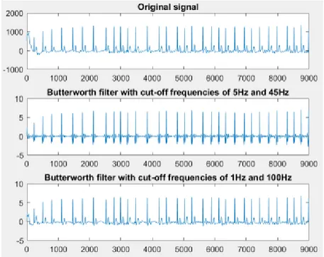
based approach which represents the spectral power of the signal and allows to detect noisy parts, since its values are higher (above 50 Hz) in frequency than parts storing cardiac information. Next the high pass filter with the cutting frequency of 0.5 Hz were added to get rid of baseline wander and a modified version of Pan-Tompkins algorithm was used for QRS detection. While in [29] authors applied logarithmic transform on the spectrogram using Tukey window with the length of 64, stating that this procedure significantly influence on classification accuracy. Others followed a bit different method in the pre-processing stage [30] using transformation into envelograms proposed in [31]. This method was based on processing signal into three types of envelopes using Fourier and Hilbert transforms. The first one corresponded to low frequency (LF) range (1-10 Hz), the second one - to medium frequency (MF) range from 5 to 25 Hz, and the third one was related to high frequency (HF) range of 50-70 Hz. Authors used this method to detect QRS by detecting the peak based on the subtraction of HF from MF resulting in automatic removal of noise from ECG signal. This approach differed from the one proposed in [32], where authors used finite impulse response bandpass filter with band limits of 3 Hz and 45 Hz and the Hamilton-Tompkins algorithm for further detection of R peaks with the subsequent PQRST templates extraction. There was additional filtering for noise or ectopic beats removal caused by some possible mistakes made by Hamilton-Tompkins algorithm. Furthermore, some studies [33] included extra step prior to the main pre-processing for avoiding imbalance in the training set by adding signals to two classes lacking of samples, i.e. AF and noisy signals. Authors of this approach padded AF class with 2000 carefully selected 10 s ECG segments from the various Physionet databases and simulated additional 2000 noisy signals as well as used time-reversing of existing noisy signals. This step is followed by filtering the signals with the 10th order bandpass Butterworth filters with cut-off frequencies of 5Hz and 45Hz (narrow band) and 1Hz to 100 Hz (wide band), and QRS detection by using gqrs [34], Pan-Tompkins (jqrs) [35], maxima search [36], and matched filtering.

As it was mentioned earlier feature extraction phase is the most significant and the derivation of relevant features determines the future classification accuracy. In comparison to the previous studies in some of the proposed techniques [28] not only features received from Poincare plots and HRV analysis were used but also morphological ECG features [33] extracted from PQRST components, prior art AF features [37] proposed by Sarkar et al [38],

(25)

25

frequency features based on Short Time Fourier Transform (STFT) and statistical features were derived. In [39] authors based their AF detection mechanism on combination of base-level and meta-base-level features including time, frequency, time-frequency, phase space and meta-level features. In addition to statistical, signal processing and medical features authors of [40] extracted features from the proposed centerwave as well as the ones derived from the Deep Neural Networks (DNN) by transforming last hidden layer values to features. Another study [37] besides some of the above mentioned features included Shannon entropy [41], K-S test values [42], the radius of the smallest circle from the normalized Lorenz plot, features based on RR intervals and similarity index between beats. On the other hand, in several approaches [29] [43] feature extraction was based on the implementation of Convolutional Neural Networks (CNN), where the model detects the significant features by its own. Finally, all of the features were fed to the corresponding succeeding classifiers.

The choice of machine learning algorithm also has a direct impact on the final accuracy. There are many factors that influence on that: the amount of implemented classifiers (either the use of only one or the ensemble of several various algorithms), the number of hidden units and layers in Artificial Neural Networks, the number and size of filters in CNN, number of batches and epochs in Recurrent Neural Networks (RNNs), kernel type and coefficient in SVM and many others. Authors who achieved the best accuracy score [44] used several stages approach. The first stage included two simultaneous trainings on extracted global and per-beat features by eXtreme Gradient Boosting of decision trees (XGBoost) and Long Short Term Memory networks (LSTMs) respectively. During the second stage, classification stacking was implemented through the combination of the probabilities from previous classifiers by means of Linear Discriminant Analysis (LDA) classifier. The implementation of various ensemble learning approaches was also seen in [40] and [28], where in the first case authors used only XGBoost algorithm to train expert, DNN and centerwave features, and adaptive boosting (AdaBoost) classifier in the second study. In some cases [29] and [43] when authors extracted features using CNN, for the classifier they employed a linear layer with SoftMax function. The implementation of Random Forest algorithm was employed by authors of [33] and [45]. Thus, in the physionet challenge among the winning approaches classification algorithms [26] extreme gradient boosting (XGBoost), Convolutional (deep) Neural Networks (CNNs) and Random Forest were broadly employed. It was noticed that

(26)

26

the given size of training data was possibly inadequate, since some of the standard classifiers, for instance Random Forest, with the carefully selected features performed as well as other more complex ones. Some small comparison of the proposed approaches is shown in the Table 2.2.

Table 2.2: The comparison of several approaches proposed in the PhysioNet/Computing in Cardiology Challenge 2017

Authors Preprocessing

techniques

Extracted features Classifiers

Datta S., Puri Ch., Mukherjee A.

et al.

Spectrogram based approach (the spectral power of the signal) for identifying noisy parts by

its power; high pass filter with the cut-off frequency of 0.5 Hz, modified version of Pan-Tompkins algorithm

for QRS detection.

More than 150 features: morphological (median, range and variance of the

corrected QT interval (QTc), QR and QRS widths

etc.), prior art AF features (AF Evidence, Original

Count, Irregularity Evidence, approximate and

sample entropy etc.), HRV features (pNNx*, SDNN**,

SDSD*** and normalized RMSSD****), frequency features (mean spectral centroid, spectral roll-off,

spectral flux), statistical features (mean, median, variance, range, kurtosis,

skewness and the probability density estimate

(PDE) of RR intervals).

Two-layer binary cascaded approach.

(27)

27 Zihlmann M., Perekrestenko D., Tschannen M. Logarithmic transform was applied on the one-sided spectrogram of the time-domain ECG signal.

Features extracted by the CNN and CRNN presented

by blocks of 4 and 6 layers were aggregated across

time. SoftMax function for calculating the class probabilities. Plesinger F., Nejedly P., Viscor I., Halamek J., Jurak P. Transformation of signals into envelograms [31] for QRS detection (LF: 1-8

Hz, MF: 5-25 Hz, HF: 45-65 Hz) and for CNN (1-5 Hz, 5-10 Hz ... 35-40

Hz).

Features were extracted from statistical description

of RR intervals as well as from the same description in

a moving window. Also some were retrieved from

CNN and correlation coefficients of average QRS. Neural Network and badged tree ensemble. Goodfellow S.D., Goodwin A. et al.

Filtering by the finite impulse response bandpass filter (limits of

3 Hz and 45 Hz), the Hamilton–Tompkins algorithm was used for R

peaks detection and was followed by additional filtering of R peaks from

any noise or ectopic beats.

Full waveform features (min, max, mean, median,

standard deviation, skew and kurtosis), templates (the

P-, Q-, R-, S-, and T-wave amplitudes and times) features (summary statistics; the PR, QS, and RT interval

times and the P-wave energy were calculated for amplitude and time of each wave), RRI features (RR

Interval (RRI), RRI velocity, RRI acceleration

and HRV features). Xtreme Gradient Boosting (XGBoost) Andreotti F., Carr O., 10th order bandpass Butterworth filters with

cut-off frequencies of

Features were extracted from HRV metrics (time domain, frequency domain

Ensemble of bagged trees (50 trees)

(28)

28 Pimentel M.

et al.

5Hz and 45Hz (narrow band) and 1Hz to 100 Hz (wide band); several QRS detectors were used: gqrs,

Pan-Tompkins (jqrs), maxima search and

matched filtering.

and non-linear features), Poincare plot and Signal Quality Indices (SQI) as well as morphological and

residual features.

and a multilayer perceptron.

* - The number of successive difference of intervals which differ by more than x ms expressed as a percentage of the total number of ECG cycles analyzed (pNNx);

** - The standard deviation of the NN intervals (SDNN);

*** - The standard deviation of differences between adjacent NN intervals (SDSD); **** - The root mean square successive difference of intervals (RMSSD).

From the table above, it is seen that the techniques implemented in the various approaches in the PhysioNet/Computing in Cardiology Challenge 2017 are more complicated than the ones discussed in the previous studies section, particularly the number of extracted features were significantly higher and the architectures of classifiers included more than one stage.

(29)

29

3 AF DETECTION IMPLEMENTATION

This chapter discusses the main steps needed for AF detection starting from the system requirements followed by the signal pre-processing, the feature extraction and the applied machine learning algorithms. It provides a comprehensive description of each of the steps in detail.

The dataset used for the experiments was used from the Physionet/CinC Challenge 2017 [26]. It comprised of 8528 single lead ECG recordings including: Normal – 5076 recordings, AF – 758 recordings, Other – 2415 recordings, Noise – 279 recordings.

3.1 The requirements for AF detection

In order to build an accurate resource-constrained AF detection tool it is crucial to specify the requirements for such system. The requirement analysis includes:

1. The proper signal pre-processing techniques should be used to remove noise and detect QRS complexes.

2. The proposed solution should extract meaningful features from ECG recordings. 3. The implemented machine learning algorithms should have relatively high accuracy

in detecting AF among 4 different types of signals.

4. The proposed solution should be computationally inexpensive. 5. The time constraint should be also taken into account.

6. The visualization of the prediction must be realized as well.

Based on the previous studies review three of the first requirements have a direct influence on the performance and accuracy of the AF detection. While the forth and the fifth ones were introduced due to the idea of the future implementation and deployment on the resource-constrained handy devices. We also introduced the last requirement as the sample visualization tool for users. All the above listed requirements will be discussed in the following sections in detail. Following these requirements, the final solution is presented as a web-based resource-constrained AF prediction system with relatively high accuracy score comparable to the current state-of-the-art.

(30)

30

3.2 Signal pre-processing: noise removal and QRS complexes detection

Since all the signals are contaminated with a noise during their recordings, first it is crucial to eliminate any kind of interferences to make further processing and analysis of the signal. The solution for the elimination of the interfering noises in the signals is the implementation of various filter types.

Based on the F. Andreotti et al. work [33], we used two 10th order bandpass Butterworth filters with cut-off frequencies of 5Hz and 45Hz (narrow band) and 1Hz to 100 Hz (wide band) respectively. Both filters remove the baseline wander noise caused by possible offset voltages in the electrodes, respiration, or body movement. By means of the first filter, QRS complexes are detected more accurately during the next step of preprocessing, since they are concentrated on 10-50 Hz range. However, besides eliminating power line interference and higher frequency noise components the first filter also removes the information about P and T wave complexes. Thus, using the second filter allows extracting features related to these complexes as well as some additional ones (residual and morphological) on later stages. The example of filtered signal having AF is illustrated on the Figure 3.1.

(31)

31

After the signals were filtered four different methods were used for QRS detection in each narrow-band preprocessed signal [33]: gqrs provided by WFBD toolbox from Physionet, Pan-Tompkins algorithm by using jqrs function (window-based peak energy detector), maxima search (for the highest peak (R complex of the signal) detection), and matched filtering (presence detection of a template signal in the unknown one by their correlation). The final reliable result of QRS detection was made by applying a voting system based on kernel density estimation.

3.3 Feature extraction

After the signal was filtered from the noise and QRS complexes were extracted, it is crucial to get the features that will carry enough information to be used for the AF detection. In our work we tried two approaches to extract features. The first one was based on the Poincare plot divided into 8 sectors, where each feature was related to the concentration of points in the sector. The second approach was based on one of the works [33] from the Phyisonet/Cinc Challenge 2017.

3.3.1 Poincare plot-based features

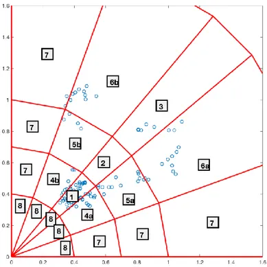
Being very practical and applicable in the AF detection among two types of signals: AF and normal, we used Poincare plot to extract features and apply them in solving our problem. Since one of the main characteristics of the AF presence is the irregularity in RR intervals, it is well reflected in the Poincare plot, where every point represents the values of the successive RR intervals (Figure 3.2). The number of points varies from the signal to signal and depends on the duration of the signal and the corresponding number of RR intervals in it. Since most of the machine learning algorithms require a fixed-size feature vector to train, we divided Poincare plot into sectors, where each of them was represented by the number of points it contained. The division was based on the relative position of the points.

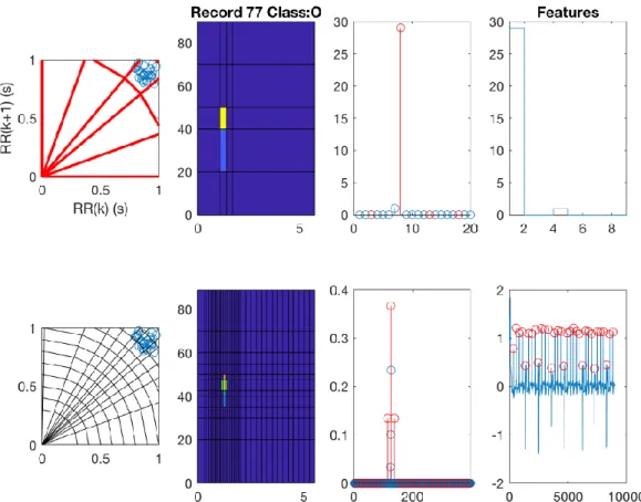
From the Figure 3.2 we can see that the signal having AF has more spread points along the main diagonal compare to the others, where the points are mostly concentrated in the central region. Therefore, we tried to extract features based on the plot division into sectors (figure 3.3). The whole process of extracting features from the divided Poincare plots is illustrated in the Figures 3.4 -3.7.

(32)

32

Figure 3.2: Poincare plot of signals having AF (left top corner), normal signal (right top corner), other signal (left bottom signal) and noisy one (right bottom corner)

(33)

33

Figure 3.4: Feature extraction for an AF signal.

(34)

34

Figure 3.6: Feature extraction for the other signal.

(35)

35

Thus, by dividing the plot into 8 sectors, the concentration of the points in each of the sectors represented each of the 8 features. In addition to 8 features, based on previous studies results [46] standard deviation of the distances of RR(i) from the lines y = x and y = -x + 2RRm, where RRm is the mean of all RR(i) were also considered as features. The ratio of two standard deviations was also calculated as a feature.

3.3.2 Extended feature extraction

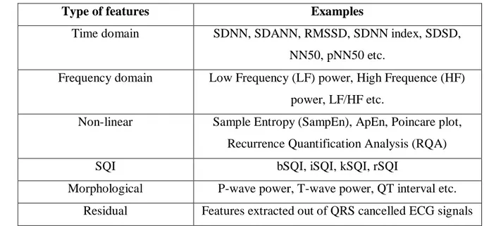
Feature extraction included [33] retrieving features from HRV analysis (time domain, frequency domain and non-linear metrics), features based on Signal Quality Indices (SQI), as well as morphological and residual features. It resulted in 171 features extracted from filtered segmented ECG signals, where the number of segments depended on the length of the recording. Therefore, for each recording the mean values across all segments were used for further processing. Some of the feature examples is shown in Table 3.1.

HRV is a variation over time of the period between consecutive heartbeats [21]. HRV analysis provides a deeper understanding of cardiac condition which can hardly be achieved by manual ECG signal examination. It is a significant tool for the detection of heart diseases, which includes several methods of analysis: time domain, frequency domain and non-linear method [14].

Time domain analysis includes two different HRV indices [21]: long term variability (LTV) and short term variability (STV), which correspond to fast and slow fluctuations in HR respectively. Both calculations are based on the RR intervals in a specified time window. Additionally, some statistical parameters may be calculated from the RR intervals: the standard deviation of the NN intervals (SDNN), the standard error, or standard error of the mean of NN intervals (SENN), the standard deviation of mean of NN intervals in 5 min (SDANN) [33], the root mean square successive difference of intervals (RMSSD), the number of successive difference of intervals which differ by more than 50 ms expressed as a percentage of the total number of ECG cycles analyzed (pNN50), the standard deviation of differences between adjacent NN intervals (SDSD).

(36)

36

Frequency domain methods are applied because of the inability of time domain analysis to discriminate between sympathetic and para-sympathetic contributions of HRV [21]. This method is related with the spectral analysis of HRV, which carries more information about the cardiac diseases presence in ECG signals. It might be concluded from the ratio of low frequency to the high frequency, which is much higher in case of cardiac abnormalities.

It was studied that signals from the non-linear living systems may be analyzed more effectively by the methods from the theory of nonlinear dynamics. These techniques include parameters like correlation dimension (CD), largest Lyapunov exponent (LLE), standard deviation (SD) relation (SD1/SD2) of Poincare plot, Approximate Entropy (ApEn), Hurst exponent, fractal dimension, a slope of DFA and recurrence quantification analysis.

Table 3.1: Extracted features

Type of features Examples

Time domain SDNN, SDANN, RMSSD, SDNN index, SDSD,

NN50, pNN50 etc.

Frequency domain Low Frequency (LF) power, High Frequence (HF) power, LF/HF etc.

Non-linear Sample Entropy (SampEn), ApEn, Poincare plot, Recurrence Quantification Analysis (RQA)

SQI bSQI, iSQI, kSQI, rSQI

Morphological P-wave power, T-wave power, QT interval etc. Residual Features extracted out of QRS cancelled ECG signals

However, extracting 171 features on the real-time predicting systems in a fast manner is highly doubtable due to computational and time constraints. Therefore, it is important to choose which features are most useful with the consideration of introduced constraints. Thus, in this work we used one of the feature selection techniques, called Recursive Feature Elimination (RFE) used for reducing the number of feature [47].

RFE is a greedy optimization technique used for finding the best performing subset of features [48]. It repeatedly builds models and keeps the worst or the best feature subsets

(37)

37

aside until all features are exhausted. Afterwards this algorithm evaluates and ranks all features based on the order of their elimination. Finally, it provides the best performed feature subset of initially specified size. We used this algorithm to reduce the number of features so that it can take less time to extract them from new signals during the operation phase. RFE implementation was realized by using provided RFE function from Python scikit-learn machine learning library [47].

In our simulations, to receive the best feature subset we trained Random Forest Classifier on the whole feature set. We varied the number of features to obtain the best feature subset ranging in size between 5 and 20 (Table 3.2). After specifying the desired size of reduced feature subset, Random Forest Classifier was trained on the whole feature set. Afterwards it assigned weights to each of them. After these steps were completed, features having the smallest weights were pruned from the feature set. This procedure was repeated on the remaining feature set until the desired number of features was reached. Table 3.2 describes only three subsets, since there was no significant difference in the training results using 15 and 20 features subsets (explained more in detail in the following chapter). And as it was mentioned by I. Guyon et al [47] the features that are chosen for the best features subset by means of their ranking are not necessarily individually most important. They perform well only in conjunction with the other features in the corresponding subset. The reduced feature subsets (5, 10, 15) included features mostly from non-linear HRV metrics, SQI based features, plus some of the residual and morphological features. On the other hand, 20 features subset also included few features from time and frequency domain HRV metrics.

Table 3.2: Top ranked features for best feature subsets

Name of a feature 5 features subset 10 features subset 15 features subset

SampleAFEv + + + RR - + + TKEO1 - + + medRR - - + iqrdRR - - + DistNext - + + ClustDistSTD - - +

(38)

38 rad2 - + - rad1rad2 + + + DistNextnS + - - rsqi3 + + - rsqi5 - - + csqi2 - - + csqi5 - + - res1 + + + res2 - - + Pheight - + - QRSpow - - + PheigtNorm - - + RRlen - - +

Figure 3.8: Plots illustrating distributions of 15 features selected by the RFE for each class in the dataset. Lines show medians. Bars depict and interquartile ranges between 25\% and 75\% percentiles. For visual purposes, the hyperbolic tangent function was applied to all

values of the features. Next, each feature was scaled using z-score method. The plots depict statistics for the scaled features.

(39)

39

Figure 3.8 presents distribution of 15 features selected by the RFE for each class. Feature numbers correspond to the order in Table 3.2. In general, not all the features demonstrate distinct separation between the classes (e.g., #2), however, it is clear that there are features (e.g., #1, #6) where classes have different values.

3.4 Implemented machine learning classification algorithms

Besides extracting meaningful features, it is also important to choose an appropriate machine learning algorithm which will detect AF highly accurately. Machine learning algorithms are recommended to use because of their ability to learn from data and make predictions on the dataset. In our proposed solution we tried several classifiers for training, however, for visualization in the web-based application, we used only two of them due to higher accuracy and better representation reasons.

Random Forest is a supervised ensemble machine learning algorithm, which uses several machine learning classifiers by building a group of decision trees. Ensemble modeling is a powerful machine learning technique for obtaining higher prediction results. According to [49] the random vectors are generated to grow the tree in the forest. Each of the trees then gives a vote for the most popular class for the given input.

Artificial Neural Network (ANN) is a computational structure [24] biologically inspired by the human brain processes. This structure is represented by highly interconnected processing units - neurons. One of the major features of ANN is “learning by example”, which increases the applicability of this algorithm in solving problems with inadequate or incomplete understanding for users. The complexity of the Neural Network, i.e. the number of layers and units in it, is fully related to the problem difficulty.

We implemented a Random Forest of 100 trees in it and a Neural Network with two hidden layers and 150 hidden units (neurons) in each of them. These parameters were empirically chosen to avoid overfitting, which may happen when the classifiers are too complex and biased to the training set. For better visualization reasons we also employed one linear layer with SoftMax function in the Neural Network classifier, which provided the activations of

(40)

40

the output layer in the form of the probability distributions. The training of the classifiers was realized with 15 features subset from Table 3.2 and 5-fold cross-validation for both and for 170 epochs for Neural Network.

The implementation of both classifiers was realized with Python machine learning libraries: scikit-learn (Random Forest) and keras (Neural Network). Both are free machine learning libraries for Python programming language. Scikit-learn is built upon the SciPy (Scientific Python), which is required to be installed beforehand [50]. This library provides a wide range of supervised and unsupervised machine learning algorithms. Keras is an open source high-level Python library for building Neural Networks, which is usually running on top of TensorFlow, Microsoft Cognitive Toolkit or Theano [51].

(41)

41

4 PERFORMANCE EVALUATION AND RESULTS

In this chapter we will first describe the performance metrics for the evaluation of the chosen approaches. Then by using the introduced metrics we will discuss how well the machine learning algorithms performed. We will also discuss whether the computations reduction realised by the feature reduction influenced the performance of the classifiers.

4.1 Performance metrics

It is highly important to choose appropriate performance metrics to properly evaluate the effectiveness of the proposed solution. One of the possible techniques for testing and evaluating machine learning algorithms is k-fold cross-validation. By means of this technique the dataset is splited into k non-overlapping subsets, where one of the k subsets is used for testing and the rest k-1 subsets form the training set [52]. Performance statistics are averaged across all k folds. It provides an indication about how well the classification will be on the new data. 5-fold cross-validation was used in our experiments and the following performance metrics were computed:

 Confusion matrix is usually used to better describe the performance of the classifier, where each row represents the instances of the actual classes and each column corresponds to the predicted ones (Figure 4.1).

 Accuracy, which shows the percentage of the correctly classified instances over the total number of instances.

 F1 score is the weighted average of the precision and recall, in the case of three and more classes classification it is an average of F1 score of each class. Precision [53] is the fraction of correctly classified instances over the total number of the retrieved instances. Recall [54] is the fraction of the relevant instances that have been retrieved over the total amount of the relevant instances.

(42)

42

Figure 4.1: Confusion matrix for four different classes (AF, Normal, Other and Noise).

Based on the presented confusion matrix, the below equations show the way of calculating the accuracy and F1 score.

The Accuracy is calculated according to the Formula 4.1.

Accuracy = 𝐴𝑎+𝑁𝑛+𝑂𝑜+𝑃𝑝

∑𝐴+∑𝑁+∑𝑂+∑𝑃

(4.1)

The final F1 score is calculated as an average of the individual F1 scores corresponding to the each of the four classes [27].

 Normal rhythm: F1n = 2 × 𝑁𝑛 ∑𝑁 + ∑𝑛 (4.2)  AF rhythm: F1a = _{∑𝐴 + ∑𝑎}2 × 𝐴𝑎 (4.3)  Other rhythm: F1o = 2 × 𝑂𝑜 ∑𝑂 + ∑𝑜

(4.4)  Noisy: F1p = 2 × 𝑃𝑝 ∑𝑃 + ∑𝑝

(4.5)  Final F1 = 𝐹1𝑛+𝐹1𝑎+𝐹1𝑜+𝐹1𝑝 4 (4.6)

(43)

43

4.2 Performance evaluation of machine learning classifiers on different feature subsets

Features obtained after the separation of Poincare plot into sectors were trained with Random Forest Classifier with 5-fold cross-validation. The results were averaged for ten simulations and are shown in Table 4.1. However, the accuracy and F1 score are quite low (0.72 and 0.55 respectively) and it is also seen in the confusion matrix (Table 4.2) that the number of misclassifications is high in all 4 classes (Table 4.2). Therefore, it was necessary to review other methods for the feature extraction. Thus, the extended feature set based on work [33] was used.

In our simulations we compared the performance of Random Forest Classifier on the best feature subsets with different sizes ranked by RFE. The performance was measured with accuracy and mean F1 score using 5-fold cross-validation. The accuracy and mean F1 score on the full set of 171 mean valued features were 0.83 and 0.75 respectively. The results (Table 4.1) showed that in comparison to the usage of all 171 features using the set of only 5 best features worsened the accuracy by 6.0 % and F1 score by 6.7 %. On the other hand, the difference to the full classifier when using 10 features was only 2.4 % and 1.3 % respectively. There was no significant performance degradation for 15 and 20 features. The subset of 15 features was chosen as the resulting one for future feature extraction from new signals and for training other classifiers. This subset was more appealing to use, since its feature extraction did not require any frequency domain computations. It included features extracted from RQA, Poincare plot, SQI metrics, 3 morphological and 2 residual features. Using only 8 features extracted from the temporal domain was comparable to 5 best features in terms of accuracy but was 7.1 % worse in terms of F1 score .

We also tried combining features derived from the Poincare plot and 171 features from [33] to see if it would increase the performance of the classifier. In some cases, more features can carry more valuable information in conjunction with each other, thus, resulting in higher accuracy and F1 score. However, in our case combining features from these two different sets did not result in any significant performance improvement (Table 4.1).

(44)

44

Table 4.1: Classification performance of Random Forest Classifier for different number of features.

Number of features Accuracy F1 score

13 (Poincare plot based) 0.72 0.55

5 0.78 0.70

8 (only time domain) 0.78 0.65

10 0.81 0.74

15 0.82 0.75

20 0.83 0.75

171 0.83 0.75

Combined 171 and 13 Poincare plot features

0.83 0.75

Table 4.2 presents the confusion matrix obtained on 5-fold cross-validation for a single run of the Random Forest Classifier trained on 13 Poincare plot based features. The cross-validation accuracy on the data was 0.72 while mean F1 score was 0.55.

Table 4.2: Confusion matrix for 13 Poincare plot based features.

Predicted

AF Normal Other Noise

Ac tu al AF 485 54 201 16 Normal 40 4532 482 20 Other 130 1153 1109 17 Noise 69 83 80 38

Table 4.3 presents the confusion matrix obtained on 5-fold cross-validation for a single run of the Random Forest Classifier trained on all 171 features. The cross-validation accuracy on the data was 0.83 while mean F1 score was 0.74.

(45)

45 Table 4.3: Confusion matrix for all 171 features.

Predicted

Table 4.4 presents the confusion matrix obtained on 5-fold cross-validation for a single run of the Random Forest Classifier trained on the best 15 features selected by RFE. The cross-validation accuracy on the data was 0.83 while mean F1 score was 0.74.

Table 4.4: Confusion matrix for 15 features selected by the RFE method.

Predicted

Tables 4.3 and 4.4 are resembling each other. Even though the performance of the classifiers was relatively high, there was still a large overlap between Normal and Other classes in the matrices. In fact, two largest sources of misclassifications are predicting instances of Normal class as Other (339 and 341respectively) and predicting instances of Other class as Normal (647 and 640 respectively). The second largest overlap is between AF and Other classes. Finally, the least represented class (Noise) gets the lowest F1 score per class. It is not surprising as the classifier is maximizing the overall accuracy, thus, it is more important to correctly classify as many as possible of the examples of the most representative class (i.e., Normal). The least representative class becomes the least important one from the point of view of the average accuracy. Note, however, that for the considered task the goal is to maximize the mean F1-score, which is negatively affected by low individual F1 scores. In

(46)

46

all tables there are many instances of Noise class which were predicted either as Normal or Other. Therefore, for the future work it will be important to improve the correctness of predicting instances from Noise class.

Additionally, we implemented an artificial Neural Network with two hidden layers and 100 hidden units (neurons) in each hidden layer. For better visualization reasons we also employed one output layer with SoftMax function, which provided the activations of the output layer in the form of the probability distributions. The training of the classifier was realized with 15 features subset for 170 epochs and with 5-fold cross-validation. However, the average accuracy (0,75) of this Neural Network was significantly lower than the one achieved by Random Forest. Nevertheless, we used this classifier, since the usage of SoftMax layer provides more detailed information about the predicted class probability of the signal.