A holistic machining line behavior modeling using Finite State Machines

(1)

1

Master Thesis

A holistic machining line behavior

modeling using Finite State Machines

Shiva Abdoli

Superviser: Dr.DanielTesfamariamSemere

December 2013

(2)

2

Abstract

Energy consumption of turning and milling operations are analyzed in this thesis profoundly. It is aimed to be able to employ analysis results in real production floors. So it is tried to investigate on most effective parameters on machine tool energy consumptions which are changeable in production floors. Due to existing limitations in predesigned manufacturing lines, cutting depth, feed rate and spindle speed, are chosen to analyze their effects on machine tools energy consumption. All other influencing parameters are presumed constant during research. Evaluating machine tools energy consumption shows increasing machining factors values reduces energy consumption in machining operation. Scrutinizing machining factors effect on energy consumption revealed that, increasing one machining factor when two other factors have constant low or constant high values has different effect on energy consumption.

The main contribution of this research is proposing a mathematical model, based on material removal rate and machining time for estimating machine tools energy consumption. In addition, a methodology to find machine energy consumption profile based on MRR in a particular operation is proposed too. This enables to find critical breakpoints of MRR for energy consumption in machining operations. Subsidiary effect of increasing Machining factors, on machine energy consumption is analyzed too. To obtain integrative conclusion regarding the effect of machining factors on energy consumption, their influence should be studied in a production system, for long term. In addition machines experience different states with different profile of energy consumption. So energy consumption of machine tools in all states is considered as product associated energy consumption. These targets are achieved by modeling a production line and simulate it for long time. The results indicates for system energy efficiency, it worth’s to increase machining factors even if tool life and consequently machine utilization reduce.

Effect of production planning such as batch mode production from energy consumption perspective in production system is evaluated. The results exhibit consistency between tool life, machine idle energy consumption and optimum batch size. The accomplishments can greatly help process planner to achieve optimum production system configuration to enhance energy efficiency.

(5)

5

Acknowledgement

Foremost, I would like to express my sincere gratitude to my supervisor Dr.Daniel Tesfamariam Semere for continuous support during my thesis research, his patience, motivation, enthusiasm, and immense knowledge.

I would like to express especial thank and love to my beloved mom and dad, you are all the reasons for me.

Last but not the least, I would like to thank my husband, your patience and love always encourage me in this way.

(6)

6

List of figures, tables and acronyms

Figures

Figure1.MRR effect on turning operation energy consumption

Figure2.MRR interaction with machining time and energy consumption in turning operation Figure3.MRR interaction with tool life in turning operation

Figure4. Tool life and energy consumption ratio in high and low experiment category in turning Figure5.MRR effect on milling operation energy consumption

Figure6.MRR interaction with machining time and energy consumption in milling operation Figure7.MRR interaction with tool life in milling operation

Figure8. Tool life and energy consumption ratio in high and low experiment category in milling Figure9. Production line model overall configuration

Figure10. Set process parameters subsystem

Figure11. Turning process parameter determination subsystem Figure12. Milling process parameter determination subsystem Figure13. Set process capability index subsystem

Figure14. Order generating subsystem Figure15. Conveyor overall configuration Figure.16 Conveyor motor controller subsystem Figure17. Conveyor, part feeder subsystem Figure18.conveyor belt subsystem

Figure19.Turnning station subsystem Figure20.Machine setup subsystem

Figure21. Machine setup flowchart subsystem Figure22. Machining subsystem in turning station

Figure23. Machining states subsystems in turning operation time Figure24. Clamping state subsystem

Figure25. Failure mode generation subsystem Figure26. Machine general state control chart Figure27. Tool life control chart

Figure28. Turning station flowchart Figure29.Milling station subsystem

(7)

7 Figure30.Gate control subsystem

Figure31.Milling station flowchart Figure32.Inspection subsystem

Figure33. Production system outputs with different MRR in milling and turning station Figure34.Tool life effect on production system

Figure35.Milling Machining factors effect on system energy consumption while turning had highest MRR

Figure36.Milling Machining factors effect on system outputs while turning had highest MRR Figure37.Turning machining factor effect on system energy consumption while Milling had highest MRR

Figure38.Turning Machining factor effect on system outputs while Milling had highest MRR Figure39.Batch mode effect on production system Energy consumption

Tables

Table 1. Different turning machining factors combination and result on energy consumption

Table 2. Regression equations for turning operation energy consumption using MRR and machining time

Table 3. Regression equations for turning operation energy consumption Table 4. Turning machining factors level on high and low extreme experiments

Table 5. Different milling machining factors combination and result on energy consumption

Table 7.Regression equations for milling operation energy consumption Table 8.Milling machining factors level on high and low extreme experiments Table9. Turning machine sections and related failure rates

Table10. failure modes occurrence probability in turning machine Table11. Turning machine sections and related failure rates Table12. failure modes occurrence probability in turning machine

Acronyms

MRR: Material removal rate FSM: finite state machine

: Process capability index

(8)

8

Chapter One: Introduction

Need for research

Global warming dilemma is intensifying nowadays, and corresponding motifs like reducing carbon dioxide emissions has been arising attention in industry. There is an unequivocal link between carbon dioxide and energy consumption. So, manufacturing industries, as huge consumer of electrical energy, should contemplate modern techniques to boost energy efficiency (1), (2).

Common goals in most production systems are increasing output, cost reduction and quality improvement (3). Energy efficient production not only helps sustainability but also benefits on cost reduction. This increases energy efficiency attitudes in manufacturing systems (4).

Realizing machines energy usage profiles and influencing parameters are the preliminary steps toward reducing machine tools energy consumption (4) (5).

Research problem

The existing models for estimating machine energy consumption mainly cover metal cutting state of one single unit. In the other hand, they mostly depend to a lot of variables. This increase model complexity and reduce their applicability. This research is motivated to accomplish an accurate mathematical model to appraise machine tools energy consumption (MTEC) based on machining factors which is also simple enough to be applicable in production floors.

In most research publications about machining operation energy consumption, the effect of various input variables has been studied on one machining operation on one single unit. But usually production plans are long term, and the effect of selecting process parameters should be investigated on mass production. In order to get comprehensive perspective in energy consumption in real production process, it is better to investigate on sequence of several types of machining operations. In this thesis a real machining process to attain a product has been studied and modeled. Each simulation run on proposed model, with different input variables is called experiment. So, it can help production planner to find the best process and system parameters configuration by comparing different experiments results.

Each particular system has its own goals which may differ from similar system. This framework can be adjusted to provide appropriate outputs. This helps to select best input parameter variables for production system, based on their prioritized goals.

Basic terms and concepts

Considering that production lines have input, output and some policies, they can be considered as system. Systems demonstrated different behavior patterns which categorizes them in different classifications. There are two typical types of systems, discrete event systems and continuous systems.

Discrete event system; ‘they have discrete-states and are event-driven and the transitions between states depend on the occurrence of asynchronous discrete events over time’ (6). Continuous systems;

inputs and outputs of these systems are capable of changing at any time instant (7). There are some systems which have both characters of discrete event systems and continuous systems, and it is hard to associate one specific type of systems to them. These systems are called hybrid systems. Production lines have some specific event and hierarchy of events like machining time. This illustrates the discrete event systems properties. But in the meantime, some event can take place in any time like failures during machining based on some stochastic functions. So it expresses some characters of continuous systems too. As a result we should consider the production line as a hybrid system, and model it with this assumption.

(9)

9

Different landscape of production goals, makes finding the best production parameters and configuration, so complicated. It is also not reasonable to find the optimum production specification by try and error in real production process. So modeling the production process and simulate its dynamic behavior can overcome this problem. Models show an abstraction of real world. So it may cover some limited aspects of real object, but it should contain main specifications. This enables to map model result in real world. Thus modeling production system benefits to reduce real experiments cost and time span to get the result. In complex problems like here with multiple objects, simulation modeling instead of analytical modeling is needed.

Finite State Machine (FSM) models the demeanor of an object. It can confront different states by transitions between states. State transition happens by satisfying some conditions like receiving some input variables or can be triggered by an event. Set of states and transitions should be finite (8), (9). State flow is widely used in hybrid systems modeling to define a discrete controller in the model. The continuous dynamics of the model are specified by using stochastic or differential equations (10). A State flow diagram is a graphical representation of a finite state machine (11). State flow can perfectly provide the interaction of continuous and discrete characteristics of hybrid systems. It mostly uses flowcharts to control the logic of a reactive system. Each state in a flowchart represents a mode of an event-driven system. Making the decision about stay in or leave from a state, investigated through the conditions. The continuous part of hybrid system can be the evaluation criteria for transition conditions. The flow charts can contain hierarchy and parallelism of states. Appropriate actions (like updating variables, calling functions, triggering events), can be defined based on the current active state of flow chart or just satisfied transition condition to move to another state. Transition actions can happen just after condition satisfaction, or after reaching the new state. The state flow in Matlab, provides plenty of options which makes the designing of flowcharts more easier and efficient, which is utilized in this thesis.

Limitation and delimitation of the study

Several parameters can affect machine tools energy consumption. Some parameters like work piece material and machine type are not changeable in production floors. They mostly depend on process limitations and customer order and the selection decision regularly are made before production planning. In the other hand in modeling perspective, increasing input variables not only increase model complexity but also reduce output accuracy. So to get better result; it is recommended to keep constant some parameters. In this thesis, it is tried to study deeply on possible changeable and measurable process parameters in production floors. As a result the investigating parameters are limited to machining factors which are spindle speed, feed and cutting depth. It is aimed to not only achieve accurate academic analysis and models, but also provide an applicable decision making framework for production floors.

Utilizing outcomes of real production line like machine energy consumption, failures and repairs times for modeling, increase model reliability. Due to all limitations to access real production line, we have to take relevant data from previous research which had been collected data from real production floors. The important issue is the research approach which won’t be affected with different input variables. Different machining operations have their own characteristics and influencing parameters but it is not possible to study all types here. Milling and turning operations which are most popular machining operations in industry, have been selected to be deeply investigated in this thesis.

(10)

10

Chapter two: Machining process characteristics

Discuss and formulate machining process parameters

Before analyzing machining factors effect on energy consumption, it is better to review some basic machining process concepts and formulas. These terms directly influence on machining operation and process parameters (12), (13), (14) (15). To avoid confusion they are described for turning and milling separately. Turning Machining time = : Cutting length : feed

: Spindle rotational speed

Material removal rate= π× × : Average diameter of work piece = ( + )/2

Material removal rate (MRR) is the volume of material which will be removed per minute from work piece with the cutting tool, it mostly expresses with /min.

Milling

Machining time= L: length of cut

ν :Linear speed of the work piece or feed rate

=extent of the cutter’s first contact with work piece which is mostly considered as half of cutter diameter

Material removal rate = wd ν

W: width of cut

: cutting depth Tool life

Tool life is considered as the useful and possible time to perform machining operation with a cutting tool. Tool wearing is the most popular failure in cutting tools (14) (16). If worn tool is used in machining operation, it not only reduces surface quality, but also increases other failures occurrence probability like tool breakage. So recognizing tool useful life and employing it just in its specified interval is a critical issue in production systems (14), (15) (16). A lot of parameters can influence on tool life, but generally it can be calculated based on Taylor formula (16), (4).

Tool life= : feed rate

(11)

11

V: cutting speed,

.d: cutting depth

C and n: work piece and cutting tool material constant

x, y depends on machining operation type and should be determined experimentally

In production floors, tool life mostly represented as the number of possible cutting operations with same tool. This term, can be regulated by dividing total tool life time to operation time (14). Number of used tools in production is another aspect of production cost associated to product.

Machine states

Machine tool faces 2 basic states; idle and busy, while there are several sub states in busy state. Considering the importance of machine busy state, and to obtain better understanding of machine tool demeanor, all sub states will be explained briefly (17) (18) (5).

Clamping: represents machine mode when clamping device start holding work piece. It refers to the changing clamping device position from un-hold to hold.

Rapid move: represents machine mode when cutting tool has a rapid motion from home position to the work piece proximity.

Spindle acceleration: represents machine mode when spindle starts rotation until reaches determined speed.

Air cutting from home position to work piece: represents machine mode when cutting tool is approaching to work piece until contact it, while spindle is rotating. This state is totally the same with machining state (cutting), but here cutting tool has not contacted the work piece yet.

Metal Machining or machining state: represents machine mode when is performing material removal operation on work piece. As soon as tool advanced to work piece, machining operation starts.

Air cutting from work piece to home position: represents machine mode when material removing operation is finished and tool slowly recedes the work piece and returns to home position. It is similar to first air cutting. When cutting tool reaches home position, the spindle motor will be turned off. De-clamping: represents machine mode when clamping device changes its position from hold to un-hold.

Failures can occur during each state of machining in different machine sections. Machine transits from busy to fail state until repair action finishes, and then transits to idle state again. It is assumed that machine will be turned off when failure happened, and switched on as soon as repair action is finished.

Process capability

Production process achieve final product by utilizing, machines, materials, staff and all other entities involved in process. The process should produce product within predefined specifications limits. Process ability to meet product specifications mostly is evaluated by statistical methods and the most popular statistical index in this area is called process capability . It clarifies the ability of under control process to perform within specification limits, by considering the inherit variability of the process. This index predicts how many parts may be produced out of specification limits (19), (20), (21).

(12)

12

Chapter Three: machine energy consumption characteristics

Analysis machine energy consumption profile

Variable & fix energy consumption

Machining energy usage profiles are mostly divided to fix and variable energy consumption. Fix energy provides machine energy requirements for operational readiness and running basic equipment features like power to start up the computer or fans. It basically depends to machine design and not affected by machining factors (17).

Variable energy consists of operational and machining energy consumption which is the required power to assure specific machining operation. This energy enables axis movement or spindle rotation, to perform air cutting operation. Machining (tool tip) energy is the power demand through material removal operation during machining process and changes by different machining factors (17).

Machine states energy consumption

As explained earlier, machine tools encounter different states in production process with different energy consumption profile. To get better realization of machine energy consumption, energy characterization of all states will be explained here briefly (17) (18) (22) (23) (4) (24) (25) (26) (5) (27)

Idle state: machine tool consumes specific and fix amount of energy during standby state, since some peripheral units are on. This energy consumption depends on machine type. The most influencing solution to reduce machine fix energy consumption is changing machine design. For instance by inactivating unnecessary features, fix energy consumption will be reduced very considerably. But it is mostly the designer job, and is not practically easy to do it in production floors. Reducing machine unproductive time contributes to reduce machine total idle energy usage and can be achieved by production plan optimization. It should be mentioned that, fix value of energy consumption will exists in all other machine states too.

Start clamping: Machine demands the peak value of power due to momentum effect since sudden change of clamping device happens to hold work piece.

Rapid move: Energy consumption of this state depends on machine energy consumption for moving each axis and the traveling path between home position and work piece place. Energy consumption can be reduced by shortening tool travelling path in this state.

Spindle acceleration: machine consumes a peak value of energy by sudden change of spindle motor due to momentum effect. Spindle motor type is the major influencing parameter on this mutation of energy consumption.

Air cutting: machine demands power in this state to move axis and rotate spindle. Spindle motor type and energy consumption due to axis movement are most influencing parameters in energy consumption in this state. Reducing tool traveling path in air cutting states can also help to reduce this state energy consumption.

Machining or metal cutting state: Machine demands power to remove material from work piece. This contributes the biggest share of energy consumption in whole machining cycle. Influencing parameters on energy consumption in this state will be investigated and analyzed deeply in next section.

(13)

13

De clamping: the energy profile of this state is totally similar with clamping action. It refers to sudden change of clamping device to release work piece. Clamping system, consumes energy in a moderate and steady mode from clamping to de clamping action for holding work piece. The practical solution to reduce this energy in production floor can be minimizing machine cycle time.

Dry and wet cutting energy concerns

Machine energy consumption in dry or wet conditions differs even all other influencing parameters are the same. Cooling operations is a considerable source of energy consumption in different forms, like cooling pump electricity consumption or cooling material usage (24) (28) (4). According to main concern of this research which is energy efficiency, dry machining operations are studied in this paper.

Analysis process parameter effect on machine energy consumption

As mentioned earlier, some influencing parameters on machine energy consumption are not changeable when dealing with existing production lines like, machine type. Cutting depth, feed rate and spindle speed are the machining variable factors which can be adjusted easier in production floors. They also determine main process characteristics like, machining time and tool life. In the other hand, by changing process parameters like tool life, they can permute machine utilization and alter machine total idle energy consumption. So, machining factors have dual effect in fix and variable energy consumption. So, in this research, the effect of machining factors will be investigated on machine energy consumption.

As explained earlier, due to all limitation it was hard to measure energy consumption in this research directly from machine tools. By studying pervious research, S.Kara presented models to estimate MTEC in turning and milling operations. The models appraise energy consumption with a good approximation (2). They are based on cutting volume and MRR in machining operation. Cutting volume is independent from cutting conditions. So it is not easy to analyze MTEC based on introduced formula. In addition, finding cutting volume may be hard in some cases, especially if there is sequence of operation in one unit. This research tries to develop an accurate model which not only gives better understanding of MTEC, but also be more applicable in production floors. So the basic model from S.kara paper is utilized to find machine energy consumption values, with different possible machining factors. Obtained energy values have been used for machine tool energy consumption analysis.

Hypothetical milling and turning operations are designed to be studied. Milling and turning are the basic operations of gear manufacturing process. Work piece material assumed to be a cold-rolled steel bar. Turning operation performs machining on work piece to reach required diameter. Process continues by milling operation to grove it. Cutting tool in milling and turning are respectively, solid-uncoated cobalt alloyed HSS and TiN coated tungsten carbide triangular inserts. Mori Seiki Dura Vertical5100 is considered for milling and Colchester Tornado A50 for turning. All tested machining factors are selected from practically possible spectrum for each factor, considering cutting tool and work piece material.

Since it is aimed to find the effect of machining factor on machine energy consumption, other parameters like, tool path in air cuttings and rapid move actions are kept constant in different machining scenarios. Milling and turning are analyzed separately in next following sections.

(14)

14 Turning

Machining factors effect analysis on machining state energy consumption

Energy consumption formulation

Table 1 shows several turning scenarios with different combination of cutting depth, feed and spindle speed. Explained formulas and relations in chapter two are used to find tool life, MRR and machining time. Taylor equation is adjusted by considering hypothetical tool and work piece material for this operation as below (15):

In table 1, Cutting depth scale is in mm, feed rate in mm per revolution, spindle speed in revolution per minute, MRR in , tool life and machining time in minute and Energy is in Mega Joule. Since number of operation with same tool is more popular in production floors, from now where ever tool life is mentioned, it refers to number of machining operations with same tool.

MRR represents all machining factors simultaneously, which are the only variables in these cutting scenarios. So, MRR is utilized to analysis machine energy consumption. Figure 1 show MRR and related energy consumption in different scenarios.

Table 1. Different turning machining factors combination and result on energy consumption

Scenarios Cutting depth Feed rate Spindle speed MRR Tool life Machining Time Number of

operation with one tool(tool life) Energy consumption A 1 0.2 500 42.4 11.9 2 5 194.76 B 1 0.14 500 29.7 15.5 2.86 5 250.96 C 1 0.2 425 36 26.7 2.35 11 218.12 D 1 0.14 425 25.2 34.9 3.36 10 284.47 E 2 0.14 500 59.3 7.74 1.43 5 157.3 F 2 0.14 425 50.4 17.5 1.68 10 173.9 G 2 0.2 425 72.1 13.4 1.18 11 140.62 H 2 0.2 500 84.8 5.93 1 5 129.05 D B C A F E G H ENERGY CONSUMPTION MRR

(15)

15

The figure exhibits increasing MRR, decreases machine energy consumption. In graph outset, small increase in MRR leads to considerable reduction in energy consumption. Energy consumption data seri expresses a reduction trend. But the slope of energy reduction by increasing MRR increases continually. In supreme section, considerable increase in MRR does not reduce energy consumption noticeably. It expresses if MRR has a substantial value, reducing one of its constitutive factor won’t have a considerable impact on energy consumption, while other remaining factors have high values. In the other hand if two of 3 factors of MRR should have low values, increasing the remaining pillar to a high value, reduces energy consumption considerably.

As mentioned earlier, considering the complexity of existing models for estimating MTEC, this research is motivated to propose an accurate but practical formula for MTEC estimation. In first chapter, it is explained that, machining time depends on MRR or machining factors. So this research, propose a formula depends on machining time and MRR which are quiet intelligible in production floors.

Using regression analysis, several estimating functions for energy consumption have developed and are showed in table 2.

Correlation coefficient (R square) in regression analysis determines goodness of linear regression model in fitting data set. This can be employed just in linear relation. But it wrongly has been used in widespread nonlinear relation regressions. (29)

refers to experimental data and is estimated data with regression model.

To be able to analysis other nonlinear regression models, modified r square for nonlinear relations has been used.

This factor assumes if the nonlinear model is a good fit, the experimental data and estimated data with model ( ) should show a good linear relation. This will be measured with above equation.

Regression Function Correlation Coefficient

Y=(0,743x+65,903)*t 0,999961 Y=(-0.00001 +0,7446x+65,865)*t 0.999963 Y=(0.00002 -0,0028 +0,8867x+63,691)*t 0.999937 Y=(0.000001 -0.0003 +0.0203 +0,1338x+ 72,28)*t 0.9925 Y=(-0.000000005 +0.000003 -0.0004 +0.0271 – 0.0278x+73.74)×t 0,9899 Y=(27.08 _)×t _0.9966

(16)

16

Second degree equation correlation coefficient is bigger than others. So it indicates better ability for estimation. The final equation for machine tool energy consumption can be express as below:

Machine tool energy consumption= (-0.00001 +0.7446MRR+65.865) × Machining time

If MTEC should have been appraised out of experimented range, depending high degree equations to more coefficients, may reduce estimation accuracy. In addition since linear equation R square has a small difference with second degree; it can be employed for MTEC estimation.

The proposed equation just depends on process parameters which are comprehensible in production floors and no need to calculate or find any extra complicated variables or constants. It also enables monitoring energy consumption during machining time, not at the end of machining operation since its time dependent. So this equation can easily be used in production floors to estimate MTEC.

Methodology for analyzing energy consumption profile

To obtain a deep understanding of MTEC relation with machining factors, equations just based on MRR are needed. This paper introduces an academic methodology to answer this requirement. It also can be easily employed in industry. The methodology includes five main steps. This methodology is applicable when, particular operation is investigated.

Step1: MTEC with different MRR should be estimated. Final equations based on MRR and time in pervious section will be used for MTEC estimation.

Step2: Several regression functions based on MRR should be regulated. These equations can be used for MTEC when the cutting volume is determined. But proposed equations in pervious section are general and can estimate MTEC for and turning operation in different cases. Table 3 proposes, estimating functions for these specific turning operations.

Step3: the best estimating function should be selected. Comparing correlation coefficients, the best fit functions for energy consumption in these specific turning operations is power equation.

Step4: second derivative equation of selected equation (power equation here) should be regulated and solved to find its roots. Recall from figure 1, energy consumption slope was negative but was increasing continuously. The acceptable root refers the point, which graph may have positive slope. In this point, by increasing MRR, energy consumption will augment. Obviously derivative equation of this power equation doesn’t have an acceptable root. All equations in table 3 are estimator functions with some estimation error. Forth degree equation has biggest R square after power equation. So, to make sure about MTEC profile, forth degree equation is analyzed here too.

_{=0, 000024} _{-0, 0318 +1,094=0}

This equation doesn’t have an acceptable root too. It apparently means MRR increment never increases MTEC in this specific operation.

Table 3. Regression equations for turning operation energy consumption

Y=-2.4561x+316,42 0.88 Y=0.048 -7,7555x+440,94 0.98 Y=-0,001 +0.2078 -15,778x+563,7 0.99 Y=0.00002 -0.0053 +0,547 -26,802x+ 689,45 0.99 Y=-0.0000007 +0. 0001 -0.0182 + 1,1844 – 41,921x+826,06 0.03846 Y=2281,8 _0,996

(17)

17

Step4: first derivative equations of selected equations (power equations) should be regulated. Root represents a breakpoint value for MRR. By increasing MRR to this value, energy consumption won’t decrease and remains constant.

=0, 00008 -0, 0159 +1,094 - 26,802=0

In turning case, first derivative equation does not have an acceptable root. It means increasing MRR always reduces MTEC. Recall, proposed methodology here is applicable only when analyzing a particular case.

Utilizing estimating MTEC models (based on MRR and time), integrated with proposed methodology, can greatly help process planner to realize MTEC. They not only can estimate MTEC in different cases, but also will achieve a deep understanding of MTEC profile in a specific operation.

Machine power demand profile

Figure 2 displays machining time and related energy consumption in different scenarios.

Cutting depth, feed rate and spindle speed constitute MRR and directly affect machining time. Figure 2 illustrate clear trends in MRR, machining time, power demand rate and MTEC. They indicate that, by increasing machining parameters, power demand rate increases in machining operation. But reduction in machining time, not only covers excessive power demand, but also reduces energy consumption in machining state. In other word to reduce energy consumption, machining parameter combination should decrease machining time.

Machining factor subsidiary effect on machine energy consumption

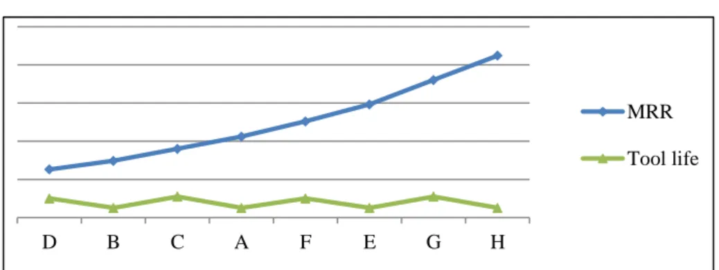
Based on analysis so far, due to reducing energy consumption in machining operation, MRR should be increased. But the subsidiary effect of MRR increment on machine energy consumption should be investigated too. As mentioned earlier, tool life is an important parameter in machining operation, since it determines number of tool replacement actions in production line. Figure 3 shows the relation between MRR and tool life. Reducing number of used tools in machining operations is another considerable target in production system. Beside tool costs, reducing number of used tools will reduce tool replacement time, which consequently increases machine available time for production.

D B C A F E G H

ENERGY CONSUMPTION Machining TIME MRR

Power demand rate

Figure2.MRR interaction with machining time and energy consumption in turning operation

(18)

18

Figure3 shows that, tool life fluctuates by increasing MRR. No explicit relation between MRR or energy consumption and tool life can be determined. MRR represents 3 machining factors simultaneously and each has different contribution on tool life Taylor equation. This clearly means same value for MRR with different values for each factor, generate different tool life. To get a deep understanding of machining factors influence on machine energy consumption, they are studied separately in next section.

Machining factors extreme analysis

To find singular effect of each machining factor on tool life, two categories of analytical experiment are arranged. They are called low extreme and high extreme experiments. Each machining factor studied in low and high extreme experiments independently. Both Low extreme and high extreme experiments include two separate internal experiments too. For example, in low extreme experiment, for each factor, two independent internal experiments are arranged. In both internal experiments no experimental factors have their lowest values. In first internal experiment, studying factor has its lowest value, and in second one has its highest value. The results of each internal experiment are related tool life and energy consumption. Correspondingly, in high extreme experiment category for each factor, two isolated internal experiments are organized. In high extreme category, no experimental factors have their highest values in both internal experiments. Experimental factor has its lowest value in first internal experiment and highest value in second one. An example makes it clearer. Spindle speed effect is studied in low extreme and high extreme experiments category independently. In low extreme experiments, feed and cutting depth have their lowest values. In first internal experiment spindle speed has its lowest value. But in second one, it has its highest value. Related tool life and energy consumption in both internal experiments are recorded. Spindle speed also is studied in two internal high extreme experiments too. Table4 displays low and high levels for each machining factor with same increment steps for all factors.

In high extreme category for each factor, the results of second internal experiment are divided to results in first internal experiment. Similarly, in low extreme category for each factor, results of second internal experiment are divided to results in first internal experiment. Each point in figure5 represents one of these dividing ratios. For example, in high extreme category of feed rate, energy consumption result when feed rate had the highest value (second internal experiment) divided to result when feed rate had its lowest value (first internal experiment).

Table 4. Turning machining factors level on high and low extreme experiments

Depth of cut Feed rate Spindle speed

0.5 0.07 212,5

1 0.14 425

D B C A F E G H

MRR Tool life

(19)

19

There are four separate data series in figure5; two series for tool life and two series for energy consumption. Each line consists of 3 points. Each point represents the ratio value (explained above) for each factor.

Energy ratios are the same for all factors in high and low extreme categories separately. It means same increase in cutting depth, spindle speed or feed rate in high or low extreme categories independently; reduces energy consumption with same ratio.

Energy consumption ratio line in low extreme is below of high extreme category. This difference means, increasing one machining factor when two other factors have their lowest values, reduces energy consumption more remarkably, comparing to situation when two other factors have their highest values.

Tool life has shown an interesting behavior in illustrated experiments in figure4. Tool life ratio from second to first internal experiment for each factor is the same for both low and high extreme categories. As mentioned earlier, tool life regulated by dividing tool operational life time (Taylor equation value), to machining time. All factors have same effect on machining time; clearly same increment in all factors, affect machining time similarly.

It is better to mention that, tool life should be an absolute value in production floors; a cutter can perform machining operation in explicit number of products, like 3 not 3.5. Due to all set up and tolerance limitations it is not acceptable practically, to stop operation in half for tool changing. So if tool life divided to machining time returns 5 or 5.2 or 5.9 tool life is 5. Since in this section, it is aimed to investigate on machining parameters interaction with tool life and energy consumption, raw value of tool life is used for analyzes.

By increasing cutting depth 2 times from 0.5 to 1 mm, tool life won’t change; tool life ratio is 1. This increment reduces tool life time 0.25 times. In the other hand it also decreases the machining time 0.25 times. So increasing cutting depth won’t have negative impact on practical tool life, while it positively reduces energy consumption in machining state.

In spindle speed the result is completely different; increasing spindle speed 2 times in both extreme categories reduces tool life 0.0625, which is tremendous reduction in practical perspective. Two reasons can justify this enormous reduction; first, the influence of spindle speed in tool life equation is considerably more than cutting depth and feed rate. Second, spindle speed value is much bigger than

3SPINDLE SPEED 3DEPTH 3FEED

ENERGY REDUCTION-low extreme

TOOL USING REDUCTION-low extreme

ENERGY REDUCTION-high extreme

TOOL USING REDUCTION-high extreme

(20)

20

feed rate and cutting depth. Spindle speed and cutting depth increase 2 times similarly. Spindle speed increase from 212.5 to 425, and the difference is 212.5. But cutting depth increase from 0.5 to 1 and the difference is 0.5. This considerable difference is also aggravated while powered in Taylor equation. So when increasing spindle speed positively reduces MTEC, reduces tool life extensively. Same results about the drastic negative effect of spindle speed on tool life (comparing to other parameters) have been achieved in other research too (26), (30), (3).

Feed rate exhibits inverse behavior on tool life comparing to spindle speed. By doubling feed rate in both categories, tool life increases 1.1 times. Feed rate has the lowest contribution effect in tool life. Feed rate from low to high value has very small difference (which is 0.07). These justify improving in tool life by increasing feed rate.

Selecting each machining factor narrows down, possible selection range for other factors. So the selection order of machining factors is a momentous task. Especially while multi targets, like energy efficiency and tool cost are pointed. All machining factors increment has same positive effect in reducing MTEC. As a result, different effect of each machining factor on tool life can determine best selection order for them.

Cutting depth and feed rate increment don’t have negative effect on tool life, while, spindle speed increment, reduces it considerably. As a result, it is better to put cutting depth and feed rate in first positions for selection and spindle speed at the end. By this order, feed rate and cutting depth can be selected as high as possible and consequently spindle speed selection range will be limited.

Feed rate increment, positively increases tool life when cutting depth won’t change it. So the first machining selection factor should be feed rate. Feed rate directly effect on Surface quality which limits its selection spectrum to meat surface quality specifications (31) (32) (33). Considering this important limitation, the biggest feed rate should be selected in machining process to take advantage of its positive effect in both energy consumption and tool cost reduction. By determining highest value for feed rate, the biggest possible cutting depth with respect to selected feed rate should be employed. Since its high value reduces energy consumption, and doesn’t affect tool life.

Selected cutting depth and feed rate restrict spindle speed selection range. This final selection depends on energy cost and tool cost preferences. In first look, if energy consumption is more important than tool cost, the highest possible spindle speed should be selected. Because it reduces MTEC positively and it’s negative effect on tool life can be neglected. But by looking deeper, new tool replacement time may have some secondary effect on MTEC in system. In this case, increasing cutting speed reduces tool life, which increases tool replacement actions. Machine is in idle state during new tool replacement actions. By increasing this action, machine total idle energy consumption increases. In the other hand, higher spindle speed reduces machining state energy consumption. So it seems by increasing spindle speed there are several tradeoffs in system dynamic perspective. This interaction will be analyzed in system analysis section and final conclusion for spindle speed value will be suggested there.

(21)

21 Milling

Machining factors effect analysis on machining state energy consumption

Energy consumption formulation

Table 5 shows different milling scenarios with different combination of cutting depth, feed and spindle speed. Explained formulas and relations in chapter two have been used to find tool life, MRR and machining time. Taylor equation is adjusted by considering hypothetical tool and work piece material for this operation as below [15]:

In table 5, Cutting depth scale is in mm, feed per tooth in mm, spindle speed in revolution per minute, Machining Time in minute and Energy is in Mega Joule.

Like turning section, MRR is utilized to analysis machine energy consumption. Figure 6 shows MRR and milling energy consumption in different scenarios.

Table 5. Different milling machining factors combination and result on energy consumption Scenarios Cutting depth Spindle speed Feed per tooth MRR Machining Time Number of operation with one tool(tool life)

Energy A 2 450 0.2 9 3.68 11 282.96 B 1 450 0.2 4.5 7.02 6 498 C 2 390 0.2 7.8 4.2 11 316.04 D 1 390 0.2 3.9 8.04 6 564.1 E 1 450 0.14 3.15 9.87 5 682.3 F 2 450 0.14 6.3 5.11 8 375.12 G 1 450 0.06 1.35 22.6 2 1 501.52 H 2 450 0.06 2.7 11.5 4 784.72 I 1 390 0.14 2.73 11.3 5 776.8 J 2 390 0.14 5.46 5.84 9 422.3 K 1 390 0.06 1.17 26 2 1 722.02 L 2 390 0.06 2.34 13.2 5 894.9 M 1 331 0.2 3.31 9.41 7 652.6 N 2 331 0.2 6.62 4.88 12 360.2 P 1 331 0.14 2.31 13.3 5 905.7 Q 2 331 0.14 4.62 6.84 9 486.8 R 1 331 0.06 0.993 30.6 2 2 016.9 S 2 331 0.06 1.99 15.8 5 1 040.4

(22)

22

Figure 5 displays MRR and energy consumption per product in different scenarios. It demonstrates reduction in energy consumption by increasing MRR.

When MRR has small value, slight increment in it, reduces energy consumption considerably. Like turning, the slope of energy reduction by increasing MRR increases continually. In graph terminal, same increase in MRR does not reduce energy consumption explicitly. It means, when all machining factors have small values, increasing one factor reduces energy consumption noticeably. But, if MRR has a high value, reducing one factor won’t increase energy consumption remarkably.

Using regression analysis, several functions for estimating energy consumption in machining state based on MRR and machining time are regulated and shown in table 6. Like turning appropriate correlation coefficient(r) are used to evaluate their estimation ability. X represents MRR and t is machining time which are independent variables and Y is energy consumption as dependent variable.

Table 6. Regression equations for milling operation energy consumption using MRR and machining time

Regression Function CorrelationCoefficient

Y=(1.4x+64.5)×t 0.985 Y=(-0.023 -1.619x+64.14)×t 0.99986 Y=(-0.001 -0.002 +1.534x+64.23) )×t 0.9999 Y=(0.004 -0.088 +0.560 -0.157x+ 65.25)×t 0.9998 Y=(-0.002 +0.061 -0.598 + 2.616 – 3.455x+67.38)×t 0.999 Y=(0.001 -0.042 +0.528 -3.252 + 10.32 -14.10x+72.7)×t 0.952 Y=(64.42 _)×t _0.8915

Comparing correlation coefficients for different equations, third degree equation shows better estimation ability here. So the final formula to calculate energy consumption of milling machine can be expressed as below:

Machine tool energy consumption= (-0.001 -0.002 +1.534MRR+64.23) ×Machining time If MTEC should have been appraised out of experimented range, depending high degree equations to more coefficients, may reduce equation accuracy for estimation. In addition since linear equation R square has a small difference with second degree; it can be employed for MTEC estimation.

Like turning, this equation depends on parameters which are comprehensible and no need to find sophisticated variables or constants. It also enables monitoring energy consumption during machining time. So this equation can easily be used in production floors to estimate MTEC.

R K G S P L H I E M D B Q J F N C A

ENERGY CONSUMPTION

MRR

(23)

23 Methodology for analyzing energy consumption profile

The explained methodology in turning is applied here too. It follows described steps in turning completely. So to avoid repetition, it is containment up to explain the results.

Several estimating functions just based on MRR are regulated and shown in table 7. Recall, these equations can just estimate energy consumption in this particular case which milling operation will remove constant volume of material. However, above equation is more general and can appraise energy consumption for milling operations with different cutting volume

Power equation, has the biggest correlation coefficients, so it shows the best ability to estimate energy consumption in this case.

Obviously derivative equations of power equation don’t have acceptable roots. Like turning to make sure about energy consumption profile, forth degree equation is analyzed here too. The roots of second derivative equation of energy consumption should be found. They represent the possible point which graph may start positive slope. In this point by increasing MRR, energy consumption will increase.

. =33.6 -376.8 +1083.9=0

This equation doesn’t have an acceptable root. It clarifies MRR increment never increases energy consumption in this case (in experimented spectrum).

First derivative equation of estimation function is regulated as below. =11.2 -188.4 +1083.9 -2079=0

4.44 is the acceptable root of this equation. By increasing MRR from pervious value to this value, energy consumption remains constant. In other word, in this point even MRR is bigger than the previous value, but the energy consumption is the same.

Realizing basic interaction between MRR and energy consumption, and integrated it with proposed methodology, conduces to find the best machining factors, to satisfy energy efficiency targets.

Machine power demand profile

Machining time and related energy consumption in different experiments is shown in figure6. Table 7. Regression equations for milling operation energy consumption

Y=-174.5x+1474 0.67 Y=45.42 -602.5x+2219 0.9083 Y=-11.12 +206.7 -1259x+2919 0.9804 Y=2.8 -62.8 +541.95 -2079x+ 3529 0.9954 Y=-0.675 +19.11 -210.7 + 1137 - 3126x+4146 0.9882 Y=0.206 -6.762 +89.22 -608.6 + 2293 -4723.4x+4944 0.991 Y=1938 _0.999

(24)

24

Like turning, by increasing MRR, machine power demand rate increases but total energy consumption reduces. This similar behavior in turning and milling can be justified through direct effect of machining factors on machining time and MRR; increasing machining factors reduce machining time, and increases MRR. Reducing machining time, not only compensate excessive power demands but also reduces total energy consumption.

Machining factor subsidiary effect on machine energy consumption

As explained earlier, increasing tool life, not only benefits directly on tool costs, but also reduces number of tool replacing actions. This reduces machine idle time and consequently machine idle energy consumption. In addition, it increases machine availability for machining operation and increases final outputs. In figure7, MRR and related tool life in different scenarios are displayed.

The graph shows considerable fluctuations by increasing MRR. This makes it hard to associate an unequivocal relation between MRR and tool life. So like turning each machining factor effect on energy consumptions and tool life is investigated in extreme experiments separately.

Machining factors extreme analysis

Like turning two levels of experiment are set, low extreme category and high extreme category. The pattern of experiments is completely similar with turning. Detailed explanation of experiments setup, is given in turning section, so to avoid repetition it is sufficient to it.

2 levels for each machining factor with same increment steps are shown in table 8. First level is called low and second level high extreme for each factor.

ENERGY CONSUMPTION MRR

Milling time Power demand rate

Figure6.MRR interaction with machining time and energy consumption in milling operation

MRR

Tool life

(25)

25

Table 8. Milling machining factors level on high and low extreme experiments Depth of cut Feed Per Tooth Spindle Speed

1 0,06 331

2 0,12 662

Tool life ratio and energy consumption from high to low extreme experiments categories is displayed in figure8.

Energy consumption ratio in low extreme category is below of high extreme for all 3 factors. This means increasing one factor to its highest value while two other factors have low values reduces energy consumption more remarkably, comparing to the situation when other factors have high values. Like turning, same increase in cutting depth, spindle speed or feed rate in high extreme category independently; reduces energy consumption with same ratio. This pattern exists in low extreme experiment category too.

Tool life ratio from second to first internal experiment for each factor is the same for both low and high extreme categories.

As mentioned in turning section, machining factors have same effect on machining time. By increasing cutting depth two times, tool life time reduces 0.9 times, while machining time reduces to half. So, tool life (number of possible operations with same tool) increases 1.8 times. Feed per tooth also has same behavior. By doubling feed per tooth; tool operational life time reduces 0.84 times, which increases tool life 1.67 times. By increasing spindle speed two times, machining time decreases to half, but tool operational life time decreases 0.4 times. As a result, tool life negatively 0.87. Different effect of each factor in tool life Taylor equation, leads to considerable difference in tool life ratios between spindle speed and two other factors.

As explained earlier, selecting each machining factor, narrows down possible range for other factors. So finding the best order to select machining factors values is a challenging task especially, when dealing with multi objective systems.

Integrating tool life analysis with energy consumption helps to find best selection sequence for machining factors in production system with energy consumption approach. All machining factors increment has same positive effect in reducing MTEC. As a result, different effect of each machining factor on tool life can determine best selection order for them.

Figure 8. Tool life and energy consumption ratio in high and low experiment category in turning

SPINDLE SPEED2 FEED2 DEPTH2

TOOL LIFE-LOW EXTREME TOOL LIFE-HIGH EXTREME ENERGY CONSUMPTION-LOW EXTREME ENERGY CONSUMPTION-HIGH EXTREME

(26)

26

Since positive effect of increasing cutting depth on tool life is more than feed per tooth and spindle speed, cutting depth should be selected first. In order to take advantage of its positive effect on energy consumption and tool life, it should be valued as high as possible.

Determining cutting depth value, limits feed per tooth possible selection spectrum. Since feed increment has dual positive effect on both on tool life and energy consumption, it should take the highest possible value too.

Feed per tooth and cutting depth values limits spindle speed selection range. Since increasing spindle speed positively reduces energy consumption and negatively reduces tool life, if energy concern was more important than tool costs, the highest possible value for it should be selected. But as mentioned in turning, new tool replacing action is affected by this parameter value. Higher spindle speed increases tool replacement actions. This increment increase machine idle energy consumption too, which may increase total energy consumption. So to find spindle speed best selection approach, its effect should be studied in a system for long time. This will be analyzed in system analysis section.

(27)

27

Chapter Four: Analytical system modeling

All above results and analysis considered machining operations on one unit in machining state, but practically production plans are long term and machine consumes energy in all states. Beside direct effect of machining factors on energy consumption, they also determine some process parameters like tool life. This can have great influence on system critical indexes like machine utilization which can probably affect energy consumptions too. Modeling production system and simulating its behavior for long time, helps to assess machining factors influence on whole system. In next section, model configuration to simulate production system is explained. It is employed for running different experiments with different input variables.

Hypothetical production system outline

To be able to analysis machining factors effect on system for long time, a hypothetical product and production line is considered and modeled.

The studying production process in this research includes turning and milling operations which are the basic sections of gear manufacturing process. Turning operation performs machining on work piece to reach required cylinder diameter. Process continues by milling to grove it and making the flutes. Beside new tool replacement and machine setup, work piece loading, unloading and machining operations, performs automatically.

Modeled production line, aimed to produce 3 product variants. Raw material comes from warehouse in first conveyor. A Robot in turning station, loads work piece form conveyor to lathe and unload it from lathe to next conveyor. In second station, there are one robot and two milling machines. Released parts from first station come in second conveyor. Robot will load work pieces to an empty machine and unload it in third conveyor. It navigates released parts to final storage. Machining time, machining setup and cutting tool life differ for each variant. So if the variant of pervious served part in machine was different from variant of coming part, machining setup should be changed.

In order to increase model consistency with real world, random failure events, random repair time and product quality rejections based on process capability are superposed in model. These features improve model resemblance with real production lines. So the results and analysis are not limited exclusively to academic research, but also is applicable for real manufacturing systems. Matlab 2013a was used to make explained production line model.

(28)

28

Model configuration

Each subsystem represents one main part of the explained production line. Subsystems contain variables, equations, flowcharts and internal subsystem to facilitate the logical flow of entities in system. These all together, contribute to provide appropriate simulation outputs. Comparing the results of different simulations (experiments) enables to analysis the effect of input variables on system.

This is the overall configuration of the model:

The model includes several main subsystems; 1-Set Process parameters subsystem 2-order generating subsystem 3-first conveyor subsystem4-turnning station subsystem4-second conveyor subsystem5-milling station subsystem 6-quality inspection subsystem 7-third conveyor subsystem8-storage block. To get better understanding of the system configuration, each subsystem will be explained separately.

(29)

29 1-Set process parameters subsystem:

This subsystem consists of three independent subsystems; turning process parameter determination,

milling process parameter determination and process capability index determination subsystem.

In turning and milling process parameters determination subsystem, depth of cut, feed and cutting speed can be set. By defining machining factors in these two subsystems and using appropriate functions, machining time, material removal rate and tool life for each variant will be calculated. These values will be sent to entity generator, milling station and turning station subsystems with connecting output ports. By changing machining factors, machining time, tool life and material removal rate will change. Machining factors are changed through different experiments in order to find and analysis their effect on system targets. It helps to find the best process parameters selection to achieve production goals.

TNU1, TNU2 and TNU3 are calculated tool life for each variant in turning operation based on

determined machining factors. MNU1, MNU2 and MNU3 are related tool life for each variant in milling operation. MRR Turning and MRR milling variables correspondingly are MRR for turning and milling operation. Turning TimeV1, V2, V3 and Milling timeV1, V2 and V3 are respectively calculated turning and milling time for each variant.

Turning process parameter determination and milling process parameter determinations subsystems

are illustrated in figures 11and 12.

(30)

30

The light green squares represent machining factors blocks. They can be changed to run different scenarios of production with different machining factors. The ovals are output variables, turning time, tool life and MRR for each variant, which will be sent to appropriate subsystems. The same structure exists in milling subsystem as well, which is illustrated in figure14, in blue theme.

Figure11. Turning process parameter determination subsystem

(31)

31

In process capability index determination subsystem we can define the process capability index (CPK).This determines the rejection probability of each part due to quality specifications (P.REJECT variable). There are plenty of options for setting CPK index. By choosing each value, the flowchart, returns appropriate rejection probability and send it to milling and turning station subsystems.

2-Entity generator subsystem:

This subsystem represents the raw material warehouse. It releases parts to production line based on customer orders. The entity generator block generates entities based on an empirical time interval too. The set attribute blocks, set variant type from1-3randomly. After setting variant type for each entity, the appropriate milling, turning and set up time for each variant should be set as an attribute. An output switch separates entities based on their variants. Milling and turning time for each variant is sent from input port of Set process parameters subsystem (Milling timeV1, V2, V3 and Turning time

V1, V2, V3 variables). Machine set up time for each variant will be set as an attribute too. When all

variant related attributes are set, a path combiner block gathers all variants together and sends them to the next subsystem, which is conveyor1.

Figure14. Order generating subsystem Figure13. Set process capability index

(32)

32 3-Conveyor1:

There are several conveyors between main subsystems. The first conveyor is between warehouse and turning station. It passes raw materials from warehouse to turning station. This subsystem contains a flowchart which checks for the availability of conveyor motor. If the motor was on, it sends a positive signal to conveyor gate (part feeder subsystem). Motor ON or OFF state is defined with a signal builder block.

.

If number of entities in buffer block (waiting parts), between machining station and conveyor was less than buffer capacity (qi conveyor variable), the block also sends a positive signal to conveyor gate (part feeder subsystem).

Figure15. conveyor overall configuration

Figure17. conveyor, part feeder subsystem Figure.16Conveyor motor controller subsystem

(33)

33

If the conveyor belt was not full and both signals were positive, the conveyor gate opens and passes new entities (the logical operator checks the positivity of both signals). An N-server block in this subsystem represents the conveyor which can pass multiple parts in the same time. If all the capacity of N-server block is full, it means that, the conveyor is full and cannot serve new part.

4-Turning station subsystem:

This subsystem represents the turning station in production line. A FIFO queue in turning subsystem represents buffer in before turning station.

Figure18.conveyor belt subsystem

(34)

34

This subsystem includes 4 main interrelating subsystems; 1- set up subsystem, 2-machining subsystem, 3- turning flowchart, 4- energy calculation subsystem. Due to existing a lot of interrelating variables, input and output ports in this subsystem, they are explained separately.

1-machine Setup subsystem

As mentioned earlier, a coming part can get the service, if machine and robot are free. There is also setup condition which needs to be satisfied. Setup action includes machining setup and tool changing. If the variant of coming part was different from the variant of pervious served part, machine needs new set up. Machine also may need a new tool, if tool life is finished. Set up action is presented in this subsystem as a single server block, and gets service time from setup time attribute of coming entity. As explained, setup attribute was defined in entity generator subsystem for each variant separately.

Machining subsystem sends signals about machine and robot availability (gate variable) by an output

port to this subsystem. The setup server also sends a signal about its state (V2 variable).If setup action is performing in machine the sending signal is 1, otherwise is 0.

Logical operator (compare to constant) in this subsystem, checks the coming signals from machining subsystem and setup server. If machine, robot and set up server were available (the signals should be zero), the logical operator generates a positive signal (out variable). It sends the signal to an enable gate block to let the entity enter to turning station.

The need for new tool replacement or new set up is checked with a flow chart. As soon as the gate opened, the robot checks the variant type (before loading). It sends variant type to the flow chart. Get attribute block in figure 20, represents this action. The machining subsystem sends tool life signal separately for each variant to this flow chart. If the coming signal about tool life was zero (life1, life2 and life 3 represents tool life for each variant), it shows that, machine can operate with existing tool; otherwise (if the signal was 1) it means, tool life is finished, and machine needs new tool to operate.