ROAD LIGHTING AND SAFETY: A PILOT STUDY OF ARTHABASKA
REGION
Mustafa Aldulaimi
MASc, Research Associate and PhD Candidate Concordia University, Montreal, QC, Canada H3G 2W1 Phone: 613-979-4324; Email: m_aldul@encs.concordia.ca
ABSTRACT
We investigate the specification of roadway lighting for safety to understand the elements needed in statistical analysis of road collisions during night time. Several goals were targeted. First, which type of response is best, or whether both responses should be used. Second, which indicator of lighting should we favor? Third, which other factors should be included in the analysis and fourth, how effective is lighting in reducing nigh-time collision. The case study comprised illuminance and luminance measurements collected for the Arthabaska region in Quebec, along with available operational and geometric variables expected to explain roadway collisions. A zero-inflated negative-binomial model was used to analyze the impact of predictors on collision frequency and severity using classical maximum likelihood validated by a Full Bayesian regression. It was found that collision severity is best, resulting in more factors being significant in the expected sense of contribution. Luminance was the best indicator for road lighting. A correlation matrix aided in the identification of linearly dependencies between factors and the response or other factors. The last goal was investigated by comparing daytime with night-time collision analysis. The night time analysis included luminance and glare. The results were very close between day and night, with luminance proving to be an effective countermeasure for night collisions. A three-time difference on the coefficient for traffic volume was found. The use of a dummy variable related to standard levels of illumination is presented and will be key in future research for the estimation of effective levels of lighting.
1.
LITERATURE REVIEW
Road collisions can negatively impact thousands of individuals. Research has proven that many severe accidents occur at night-time (Isebrands et al. 2010, CIE 1992), particularly involving pedestrians (Zhou and Hsu 2009).The typical countermeasure for night-time collisions is roadway lighting (Rea, Bullough, and Zhou 2009). Studies have observed significant reductions in night-time collisions at road segments to which lighting was provided as a countermeasure, with effectiveness ranging between 10 to 40% of all crashes observed and up to 65% of fatal crashes (TAC 2004). Previous research has found a roughly 37% reduction of crash rates (Isebrands et al. 2010). This is also supported by a report by CIE (CIE 1992) that found a large number of studies before 1992 which revealed that night-time accidents resulted in more severe accidents and that lighting did help reduce their frequency. Several studies have been conducted to examine the relationship between roadway lighting levels and safety. Some researchers (Isebrands et al. 2010, Zhou and Hsu 2009) investigated how maintained illuminance levels impact safety of pedestrians, finding a higher frequency of pedestrian crashes at sites with low level of lighting. Others found that road lighting contributes to reduce collision frequency and especially reduce the number of persons killed and seriously injured (Yannis, Kondyli, and Mitzalis 2013).
The majority of studies on lighting refer to illuminance of a single site. Illuminance portable technology has recently been developed (Cai and Li 2014). Measurement of luminance for road safety studies of nigh-time crashes is recent. Luminance portable technology does exist but has been impractical for collecting massive amounts of data (Elvik 1995).
2.
MOTIVATION AND GOALS
The main motivation of this paper is to explore the role of lighting as a countermeasure for night-time road collisions involving motorized vehicles in road segments. Several aspects need to be studied or confirmed. First, whether severity and/or frequency is the best response to capture the causes of night time collisions in statistical analyses. Second, what indicator of lighting should be used for road segments, illuminance or luminance. Third, what geometric, functional, and operational characteristics of the segment should be used as causal factors. Fourth, to confirm that lighting is indeed a good countermeasure.
As expected, the main goals respond directly to each of the four previous aspects. In summary, this paper identifies what response should be used, what factors were considered and what indicator of lighting was included, and finally, the effectiveness of lighting as a countermeasure as witnessed through a reduction in collision rates. Good understanding for the specification of statistical analyses will be developed.
3.
THE DATABASE
Part of the data used in the first part of this research was obtained from the Arthabaska region. These databases benefitted from the work of a team of students under the supervision of Dr. Nicholas Saunier of Ecole Polytechnique, that merged the spatial location from the emergency vehicle system to the one of the Ministry of Transportation, this signified the ability to count with a more precise spatial location of the accidents which in turn justifies the possibility to use segments of 100 meters. A total of 951 road segments of 100 meters were used in this pilot study. Some geometric and operational characteristics of the segments along with lighting measurements, accident counts, and a severity index were used for the analysis. Geometry attributes included presence of intersection, number of lanes, complex geometry, posted speed, land use (i.e. rural or urban), and average AADT for a period of ten years.
Roadway lighting in the form of illuminance and luminance was collected for a network of around a 95 km of roads in the Arthabaska region in central Quebec (Figure 1). Illuminance measurements were collected using the Spectrosense2+ machine by placing two light sensors on top of the roof of a passenger car along with the device’s built-in GPS system. An additional assisted-GPS was used to input missing coordinates in those cases where the Spectrosense2+ lose signal.
Figure 1: Arthabaska Region and Highways on This Pilot Study.
A protocol for data collection is presented in (Figure 2). Data collection begins and ends with the drivers being at a stationary position in order to have a known location and to allow the GPS to find signal; the driver then proceeds at near constant speed in order to have uniform point separation. Data collection is complemented by a cleaning process during the processing to remove measurements logged while stopped. Spectrosense2+ and the assisted GPS have to be turned on and off simultaneously at the commencement and at the end of data collection respectively. The data then needs to be transferred to a computer system where it is processed.
A preliminary visual inspection of the data is done using ArcGIS, where missing data can be easily identified. Coordinates from the assisted GPS are added in such cases. The complete cleaned illuminance dataset is then saved as a shape file which will be used at a later stage.
In terms of Luminance, data was collected using a professional digital camera (Nikon D70) with a special lens filter (fish eye type) and specialized software capable of estimating average luminance from ISO 400 photos as perceived by the driver and a glare indicator (Photolux 2012). Data collection followed the parameters established by JIS-Z-9111 (1988) in terms of the location of the camera (midpoint between luminaires), angle (2 degrees from horizontal sight of driver), height (1.5m), visual environment (capturing distance between 60 and 160 meters ahead, 90 m for intersections) and other specifications related to data collection already predefined in the system. Jackett and Frith (2013) further explained the calibration of a commercial camera required to translate photo pixels into luminance values. One indicator of glare was tested; the unified glare ratio.
Photolux software was used to process pictures by reading the information stored in the header of the picture using the EXIF format (Photolux 2012). This information includes the aperture, time of exposure, and sensitivity. Photolux computes the exposure used on the picture to assign a value of luminance to each pixel, which eventually results in a luminance map. This map represents the amount of luminance in candela per square meter and can be used to estimate glare indicators.
A second subprocess takes care of adding the road network’s operational and geometric characteristics and splits roads into one hundred meter segments. In addition, intersections were
identified by creating buffers. Segmentation of the network followed a two-step process where routes were created and divided. The creation and splitting of the routes resulted in the loss of relevant segment-related attributes. Characteristics corresponding to each section are reincorporated into the splitted segments shapefile.
A third process uses a 20m buffer to allocate collisions into road segments in the form of collision frequency and by using specified weights (3.9, 1, 0.0216, 0.0108 and 0.0014 for fatality, major/minor, injury and major/minor PDO) creates a severity indicator scaled to match the order of magnitude of observed frequencies. Finally, lighting measurements, road network operational and geometrical characteristics, and accident frequency were joined together. The final database was used for statistical analyses (Figure 2).
Data Collection Illuminance D at a Pr oc es si ng
Cleaning, & removal of a lighting logged while
stopped Preliminary Visualization in ARCGIS Missing data? Inputting missing coordinates Convert to shapefile (point format)
Isolate road network (line format)
Identify intersections and create buffers
Create routes for same road name/number
Split routes into 100m, and bring road
network
Open accident data in ARCGIS
Road Network (Operation and geometry)
Add attribute column with value 1
JOIN SUM of accident data into 100m segments to generate accident count
per segment
JOIN network with accidents to Lighting. Use Average, Maximum and Minimum Statistical Analysis Stata Spectrosense Assisted GPS Cleaning Preliminary Visualization in ARCGIS Calculating the Light Parameters Convert to shapefile (point format)
Roadway Lighting Measurement
Historical Road Collisions
YES NO Creating Luminance Map using Photolux Data Collection Luminance Assisted GPS Digital Camera Luminance Part Illuminance Part
4.
LIGHTING VARIABLES USED IN THE ANALYSIS
Values of uniformity followed those recommended by IESNA (2005) which defines uniformity of illuminance or luminance as shown on Equations 2, 3 and 4.
Uniformity (illuminance) Minimum Average [2] Uniformity (luminance)
Average
Maximum
[3] Uniformity 2 (luminance) Minimum Average [4]According to IESNA (2005), the uniformity ratios are dependent on the functional classification of the road. The values provided in this table are the maximum allowable values that can be observed on road segments. Road segments in the database were classified as being standard by looking into the minimum illuminance and luminance values and functional classification in order to meet IESNA minimum recommended illuminance and luminance values. Uniformities for illuminance and luminance were used in the analysis as well. Average illuminance and calculated uniformity were the only light related variables used in the analysis. A dummy variable for lighting levels describing whether the light found on the segment is standard or non-standard was included as well. The natural logarithm of AADT has been chosen as a predictor to inflate the regression. This is because the number of crashes (or their severity) is related to traffic volume (AADT), i.e., many segments with low levels of traffic registered zero collisions.
5.
METHODOLOGY
This first stage of the analysis develops frequency and severity statistical models for roadway collisions in order to identify the recommended form of the response. The analysis is conducted in two parts: one for lighting in the form of illuminance and the other in the form of luminance. Maximum likelihood and Full Bayesian analyses were employed (the second to validate the results of the first) to identify the factors that are significant. The main tasks are shown on (Table 1).
Table 1: Main Tasks
Method Purpose
Statistical analyses of collision’s frequency and severity Identify best type of response
Statistical analyses of illuminance and luminance Identify best indicator for lighting
Correlation Matrix Identify causal factors to be used
Statistical analyses of daytime vrs. night-time collisions Demonstrate lighting is countermeasure
Full Bayesian and maximum likelihood Validation of results
6.
STATISTICAL ANALYSES
Different methods are available to estimate the parameters of a regression model. The most popular in safety analysis are the method of moments (Baglivo 2004), the method of maximum likelihood (Bedford and Cooke 2001), and Bayesian estimation (Gelman and Hill 2008). The method of maximum likelihood is widely accepted, and therefore used in this study. However, Full Bayesian counts with interesting properties and interpretive advantages (Mitra and Washington 2006) like the ability to handle structured data which could be exploited to replicate the ideas behind Latent class models and to abandon the need to inflate for zeros.
The analysis in this paper runs parallel models with maximum likelihood as the main method and Full Bayesian in order to validate its results. However, Bayesian analyses will be the base of future
research in order to develop a calibration method that separates road sites by levels of risk and then establishes calibrated lighting warrants.
A Zero-Inflated Negative-Binomial (ZINB) model is used to estimate the contribution of explanatory variables (including lighting) on collision frequency and severity. The ZINB is an extension to the ZIP, capable of dealing with the high number of zero counts as well as over-dispersion (Mei-ling et al. 2004). This model assumes that the high number of zero responses could come from two possible processes. One could be the result of good safety practices and adequate geometric design. The second could come from some collisions not being reported. The outcome Y studied herein follows a ZINB with distributions and the mean for the variance as recommended by Sharma and Landge (2013).
This paper employs a safety performance function (SPF) that estimates the relationship between predicted crash frequency and a series of segment characteristics from four major areas, namely operational characteristics (AADT, speed, et cetera), geometry and built environment (land use, curvature, et cetera), environmental exposure (road surface condition), and roadway illumination. The SPF adopted in this study is presented in (Equation 1) and follows the format recommended by AASHTO (AASHTO 2010). It should be noted that all segments measure 100m in length making possible to drop such factor.
+ [1]
Where:
k : variable number (1,2,3,….)
βk : Coefficient of explanatory variable
: Frequency or severity of night-time collisions on segments i AADTi : Average Annual Daily Traffic of segments i
Xki : Explanatory variable i
α : Coefficient of AADT at segment i
7.
RESULTS
An increase in the number of collisions is expected for high traffic areas. Two models were run: classical analysis (maximum likelihood) using Stata and Full Bayesian using OpenBUGS (Table 2).
7.1. Road Collisions and illuminance
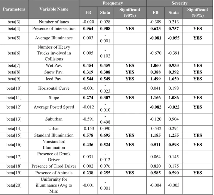
A zero inflated negative binomial model was analyzed using a maximum-likelihood commercial-software (Stata) and a Full-Bayesian free-source-commercial-software (OpenBUGS). Two sub-models were prepared and results were obtained; one for accident frequency and one for accident severity. Their results were compared in (Table 2) in order to validate and to withdraw conclusions regarding the preferred response.
The presence of an intersection, having a wet, icy or snowed pavement, along with the slope of the terrain and the presence of animals increase the number of roadway collisions. Higher average speeds resulted in slightly less accidents with an almost negligible contribution. More causal factors were capable of explaining accident severity; as such and in addition to the aforementioned variables, higher levels of average illuminance were found to explain less severe accidents. The presence of animals increase the frequency and severity of collisions. Tired and drunk drivers resulted insignificant for explaining collisions frequency and severity. Sites with standard levels of illumination were associated with more severe accidents as compared to sites with non-standard levels. This contradictory result aligns with the literature recommendation of not using illuminance as an indicator for road segments (only for intersections). This also suggests the possibility that the current standard is not helping to reduce the number of road collisions and may need to be revised.
Table 2: Comparison Maximum Likelihood (Stata) with Full Bayesian (OpenBUGS) for Illuminance
Parameters Variable Name
Frequency Severity FB Stata Significant
(90%) FB Stata
Significant (90%)
beta[3] Number of lanes -0.020 0.028 -0.309 0.213
beta[4] Presence of Intersection 0.964 0.908 YES 0.623 0.757 YES
beta[5] Average Illuminance 0.003
-0.001 -0.081 -0.055 YES beta[6] Number of Heavy Trucks involved in Collisions 0.005 -0.102 -0.670 -0.391
beta[7] Wet Pav. 0.454 0.459 YES 1.060 0.933 YES
beta[8] Snow Pav. 0.319 0.308 YES 0.388 0.392 YES
beta[9] Iced Pav. 0.544 0.549 YES 1.499 1.650 YES
beta[10] Horizontal Curve -0.001
-0.023 0.041 0.198
beta[11] Slope 0.274 0.307 YES 1.166 1.086 YES
beta[12] Average Posted Speed -0.012
-0.010 -0.082 -0.022 YES
beta[13] Suburban -0.591
-0.498 -0.120 0.904
beta[14] Urban -0.153 0.090 -0.542 0.294
beta[15] Standard Illumination 0.578 0.695 YES 1.185 1.255 YES
beta[16] Nonstandard
Illumination 0.436 0.524 YES 0.511 0.598 YES
beta[17] Presence of Drunk
Driver 0.031
-0.012 0.064 0.145
beta[18] Presence of Tired Driver 0.002 0.076 0.820 0.175
beta[19] Presence of Animals 0.238 0.255 YES 0.585 0.590 YES
beta[20] Uniformity for illuminance (Avg to Min) -0.001 -0.001 -0.004 -0.003
7.2. Road Collisions and luminance
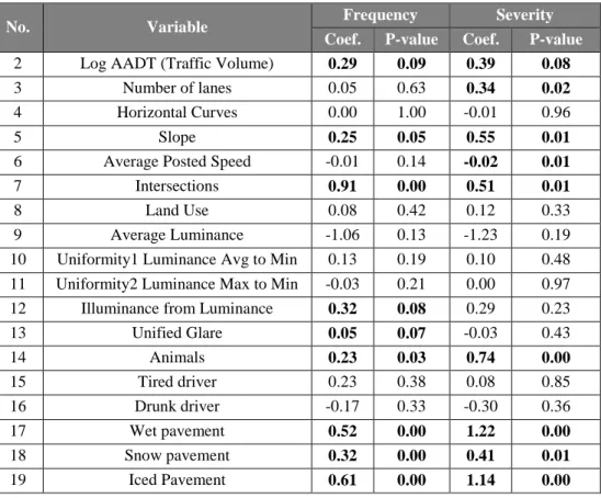
In this analysis, lighting took the form of luminance and glare (unified), for the same segments used in the analysis before. It was confirmed that segments with higher levels of traffic flow, on a slope, at an intersection, or exposed to slippery circumstances or the presence of animals (possibly poor fencing control) experienced a higher number of accidents. In terms of lighting, this analysis measured the role of luminance as perceived by the driver, glare, and uniformity variation (the higher the value the larger the lighting inconsistency). It was found that higher values of luminance resulted in less frequent and severe accidents (although at an 85 and 80% confidence), higher values of glare resulted in more frequent collisions and higher degrees of inconsistency in uniformity, resulting in more collisions. Tired and drunk drivers resulted insignificant for explaining collisions frequency and severity (Table 3).
Table 3: Classical Analysis (Maximum Likelihood) Analysis Results – Stata
No. Variable Frequency Severity Coef. P-value Coef. P-value
2 Log AADT (Traffic Volume) 0.29 0.09 0.39 0.08
3 Number of lanes 0.05 0.63 0.34 0.02
4 Horizontal Curves 0.00 1.00 -0.01 0.96
5 Slope 0.25 0.05 0.55 0.01
6 Average Posted Speed -0.01 0.14 -0.02 0.01
7 Intersections 0.91 0.00 0.51 0.01
8 Land Use 0.08 0.42 0.12 0.33
9 Average Luminance -1.06 0.13 -1.23 0.19
10 Uniformity1 Luminance Avg to Min 0.13 0.19 0.10 0.48 11 Uniformity2 Luminance Max to Min -0.03 0.21 0.00 0.97
12 Illuminance from Luminance 0.32 0.08 0.29 0.23
13 Unified Glare 0.05 0.07 -0.03 0.43 14 Animals 0.23 0.03 0.74 0.00 15 Tired driver 0.23 0.38 0.08 0.85 16 Drunk driver -0.17 0.33 -0.30 0.36 17 Wet pavement 0.52 0.00 1.22 0.00 18 Snow pavement 0.32 0.00 0.41 0.01 19 Iced Pavement 0.61 0.00 1.14 0.00
7.3. Causal factor selection
The previous analyses were not concerned with the selection of factors and concentrated only on the identification of the ideal response(s) and suitable indicator(s) of lighting. This section is devoted to the identification of the causal factors to include in the analysis. The prior belief is that any factor in principle correlated to the response should be dropped. By correlated in principle, one means those who represent a specific characteristic of the response. For instance in the previous analysis, the presence of an animal at the time of the accident is a count of how many of the observed accidents involved an animal; similarly the impairment of the driver (tired or drunk) is also a mere count of accidents in which the driver presented as either of those circumstances. Finally, the surface of the pavement at the time of the accident is also a mere count of frequency of how many accidents occurred while the surface of the pavement presented some wet, icy, or snowy circumstances.
Table 4: Correlation Matrix for In-Principle Correlated Factors
y = frequency Animal Driver Pavement Tired Drunk Wet Snow Ice
y = frequency 1 Animal 0.31 1 Tired 0.17 0.13 1 Drunk 0.39 0.30 0.57 1 Wet pavement 0.88 0.22 0.15 0.33 1 Snow pavement 0.79 0.30 0.18 0.30 0.59 1 Ice pavement 0.51 0.18 0.14 0.26 0.30 0.37 1
(Table 4) shows a portion of a correlation matrix of such factors with accident frequency, while the other portion containing the remaining factors is shown on (Table 4) given the large size of the matrix. As seen, most accidents presented a slippery circumstance, about half involved an impaired
driver, and one third involved the presence of an animal on the road. They all result in high values of correlation and should not be included in the analysis.
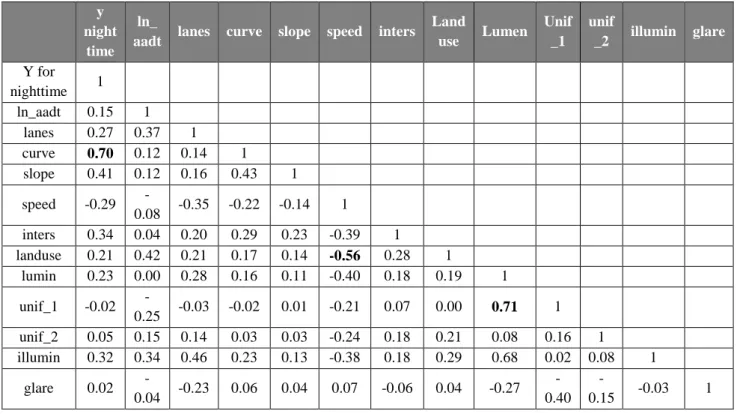
As seen in (Table 5) there are three factors showing high values of correlation one of them (horizontal curve) with the response possibly because such measure (binary) only reflects the fact of whether the collision occurred at a horizontal curve segment or not. If this is the case, such geometric variable is inadequate and one containing the actual measure of the radius of curvature should be used. The other two variables showing high correlation are land use with speed (56%) and illuminance with luminance (68%). The reasons behind the second pair of highly correlated factors (illuminance and luminance) are very clear; the value of illuminance was estimated from the value of luminance, and hence only one or the other should be used. A negative correlation is observed between speed and land use, which means the more types of proximal land uses (urban and suburban) to a road segment, the lower the observed speed. This observation makes sense as the indicator of land use herein defined acknowledges the fact that homogeneous circumstances (only one type of land use) possibly results in higher speeds, and that transitioning segments will likely observe lower speeds.
Table 5: Correlations for the rest of causal factors
y night
time ln_
aadt lanes curve slope speed inters
Land use Lumen Unif _1 unif _2 illumin glare Y for nighttime 1 ln_aadt 0.15 1 lanes 0.27 0.37 1 curve 0.70 0.12 0.14 1 slope 0.41 0.12 0.16 0.43 1 speed -0.29 -0.08 -0.35 -0.22 -0.14 1 inters 0.34 0.04 0.20 0.29 0.23 -0.39 1 landuse 0.21 0.42 0.21 0.17 0.14 -0.56 0.28 1 lumin 0.23 0.00 0.28 0.16 0.11 -0.40 0.18 0.19 1 unif_1 -0.02 -0.25 -0.03 -0.02 0.01 -0.21 0.07 0.00 0.71 1 unif_2 0.05 0.15 0.14 0.03 0.03 -0.24 0.18 0.21 0.08 0.16 1 illumin 0.32 0.34 0.46 0.23 0.13 -0.38 0.18 0.29 0.68 0.02 0.08 1 glare 0.02 -0.04 -0.23 0.06 0.04 0.07 -0.06 0.04 -0.27 -0.40 -0.15 -0.03 1
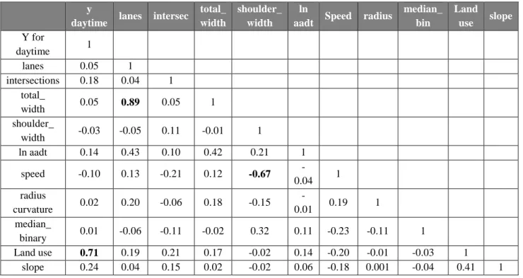
Table 6: Correlations for the causal factors on daytime analysis
y
daytime lanes intersec
total_ width
shoulder_ width
ln
aadt Speed radius
median_ bin Land use slope Y for daytime 1 lanes 0.05 1 intersections 0.18 0.04 1 total_ width 0.05 0.89 0.05 1 shoulder_ width -0.03 -0.05 0.11 -0.01 1 ln aadt 0.14 0.43 0.10 0.42 0.21 1 speed -0.10 0.13 -0.21 0.12 -0.67 -0.04 1 radius curvature 0.02 0.20 -0.06 0.18 -0.15 -0.01 0.19 1 median_ binary 0.01 -0.06 -0.11 -0.02 0.32 0.11 -0.23 -0.11 1 Land use 0.71 0.19 0.21 0.17 -0.02 0.14 -0.20 -0.01 -0.03 1 slope 0.24 0.04 0.15 0.02 -0.02 0.06 -0.18 0.001 -0.04 0.41 1
7.4. Demonstrating that Lighting is a Countermeasure
The analysis, however, is based on an expanded version of the database which contained more segments (1600 segments) with geometric values for lane width, number of lanes, total pavement width, shoulder width, slope, horizontal curve radius, density of intersections/interchanges, and traffic volume. The data contained for land use on the database showed a high (0.71) correlation coefficient with the response (Table 6). The reason was that the fields of land use in the database reflected a count of collisions observed at the corresponding land use, so for this reason it was dropped from the analysis. The same correlation matrix (Table 6) revealed that total width was highly correlated to number of lanes. Only one value was kept for the analysis.
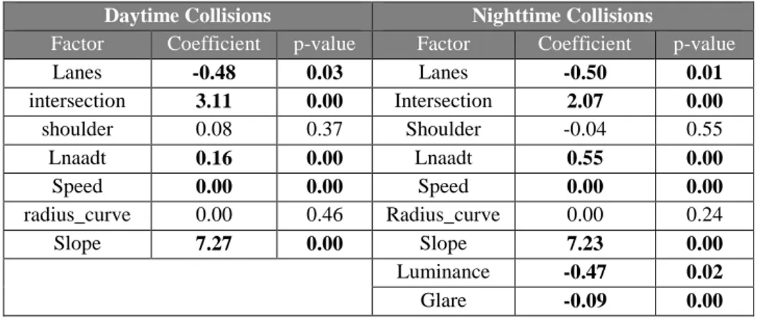
Lighting was represented by luminance and glare, collision severity was used as response. As seen in (Table 7), both daytime and nighttime identify the same significant factors: number of lanes, density of intersections, traffic volume (AADT), posted speed, and slope. All coefficients are very close except the one for traffic volume which is about three times as important during nighttime. This could be explained by the fact that traffic volume has a greater impact on night time accidents. This is seen in the warrant score system of highway lighting by the use of a 2 to 1 night-to-day accident ratio. Both luminance and glare resulted significant and negative, which is to say that higher luminance and glare result in fewer collisions. This confirms that for the case study, lighting measured through luminance is an effective countermeasure. The result for glare contradicts prior expectations, thus glare should not be used.
Table 7 Day and night time analyses
Daytime Collisions Nighttime Collisions
Factor Coefficient p-value Factor Coefficient p-value
Lanes -0.48 0.03 Lanes -0.50 0.01 intersection 3.11 0.00 Intersection 2.07 0.00 shoulder 0.08 0.37 Shoulder -0.04 0.55 Lnaadt 0.16 0.00 Lnaadt 0.55 0.00 Speed 0.00 0.00 Speed 0.00 0.00 radius_curve 0.00 0.46 Radius_curve 0.00 0.24 Slope 7.27 0.00 Slope 7.23 0.00 Luminance -0.47 0.02 Glare -0.09 0.00
8.
CONCLUSIONS
This research presented a protocol to collect lighting data and developed understanding of the role of lighting in explaining night-time collisions. This will be used in future research to develop a method to calibrate lighting warrants and design levels. In terms of the four major goals of this research, results from the analysis showed that accident severity is preferred over frequency, but one should keep in mind that they respond to different circumstances and it is the opinion of the author that both should be kept in the analysis. It was observed that illuminance returned inconsistent values for the statistical analysis of collisions on road segments, whereas luminance showed strong significance and improvement as a countermeasure. This result aligns with the literature that recommends the use of luminance for road segments (no pedestrians). Correlation analyses proved useful in identifying linearity between factors (same nature) or between factors and the response.
Miscellaneous initial results showed that, for the Arthabaska region in Quebec, the presence of an intersection, the presence of animals, and having a slippery/wet road surface produced more frequent and severe collisions. However, the correlation analyses force the drop of the presence of animals and slippery/wet roads as well as driver impairment. Roads with complex alignments resulted in higher collision rates. Traffic volume also explained higher collision frequency. Standard illuminated roads resulted in an increase of road collision frequency, a contradictory result. Average level of illumination (and being at an urban location) was only significant from a severity perspective, explaining less severe accidents with higher levels of illumination.
It was confirmed that Full Bayesian analysis was capable of estimating the impact of the explanatory variables on the response as it returned similar results to those obtained by the classical analysis. This is a key step for the validation of statistical analyses using Full Bayesian analysis. Future steps of this project include the development of a method to calibrate lighting warrants and estimate recommended design levels of lighting indicators. Such specifications will be based upon refined statistical analysis containing all the recommendations found in this paper.
9.
REFERENCES
1. American Association of State Highway Transportation Officials. Highway Safety Manual: AASHTO, Washington D.C., USA, 2010.
2. Baglivo, J. A. Mathematica laboratories for mathematical statistics. Society for Industrial & Applied Mathematics. Philadelphia, USA, 2004.
3. Bedford, T., Cooke Research Carried Out for the AA Foundation for Road Safety Research
and the County Surveyors’ Society. Available at:
http://www.roadsafetyfoundation.org/media/11323/aa_foundation_fdn34.pdf, accessed on August 05, 2013.
4. Cai, H. and Li, L. 2014. Measuring Light and geometry data of roadway environments with a camera. Journal of Transportation Technologies. pp. 44-62
5. CIE. International Commission on Illumination: Road Lighting as an Accident Countermeasure. Austria: Research Report CIE093-1992, 1992
6. Elvik, R., Meta-Analysis of Evaluations of Public Lighting as Accident Countermeasure. Transportation Research Record No.1485, Transportation Research Board of the National Academies, National Research Council, D.C., pp. 112-123, 1995.
7. Gelman, A., Hill, J. Data analysis using regression and multilevel/hierarchical models. Cambridge University Press. Cambridge, UK, 2008
8. Illuminating Engineering Society of North America. Roadway Lighting: American Standard Practice for Roadway Lighting. New York: IESNA Publication; Report RP-08-00, 2005 9. Isebrands, H.N., Hallmark, S.L., Li, W., McDonald, T., Storm, R. and Preston, H. Roadway
Lighting shows safety benefits at rural intersections. Journal of Transportation Engineering. Vol 36, No. 11. pp. 949 – 955, 2010.
10. Jackett, M., Consulting, J., and Firth, W. How does the level of road lighting affect crashes in New Zealand-– A pilot study. New Zealand Transport Agency, 2012
11. JSA. Japanese Standard Association: Japanese Industrial Standard of Lighting for Roads JIS Z 911, 1988
12. Lord, D. and Persuad, B. N. Accident Prediction Models With and Without Trend: Application of the Generalized Estimating Equations Procedure. Transportation Research Record: Journal of the Transportation Research Board; 1717: pp. 102-108, 2000.
13. Mitra, S., Washington, S. On the nature of over-dispersion in motor vehicle crash prediction models. Accident Analysis and Prevention. 39, pp. 459–468, 2006.
14. Mei-ling, S., Hu, T.W., Keeler, T.E., Ong, M., and Sung, Y. The Effect of a Major Cigarette Price Change on Smoking Behavior in California: A Zero-Inflated Negative Binomial Model. Health Economics; 13(8): pp. 781-791, 2004.
15. Photolux, 2012. Photolux 3.2 User’s Guide [online]. Soft energy consultants. Available at
http://www.photolux-luminance.com/images/stories/photolux/download/Photolux_public_lighting_3_2_Users_guid e_Eng. pdf [December 27 2013]
16. Rea, M.S., Bullough, J.D. and Zhou, Y. A method for assessing the visibility benefits of roadway lighting. Lighting Research Technology. No. 42. pp. 215-241, 2009.
17. Sharma, A.K., Landge, V.S. Zero Inflated Negative Binomial for Modeling Heavy Vehicle Crash Rate on Indian Rural Highway. International Journal of Advances in Engineering & Technology, 2013.
18. Transportation Association of Canada. The Canadian Guide to In-Service Road Safety Reviews. Ottawa Canada: TAC Publications, 2004.
19. Yannis, G. Kondyli, A. and Mitzalis, N. Proceedings of the Institution of Civil engineers, Transport 166, Issue TR5. pp. 271-281, 2013.
20. Zhou, H. and Hsu, P. Effects of roadway lighting level on the Pedestrian Safety. On Critical