Research
Slow strain rate testing of copper
in sulfide rich chloride containing
deoxygenated water at 90 °C
2017:02
Authors: Richard Becker Johan Öijerholm
SSM perspective
BackgroundStress corrosion cracking (SCC) can occur in materials from the
com-bined influence of tensile stress and a corrosive environment. It has
previously been shown in the literature, that copper can be sensitive
to SCC in the presence of sulfide containing water. Since both tensile
stresses are present as well as a material were SCC can occur, SCC could
potentially be a problem for the copper canisters intended to be used
for final storage of spent nuclear fuel.
Testing materials susceptibility of SCC can be performed by
accelerat-ing the tensile stresses, the environment or both. A testaccelerat-ing method
fre-quently used within the nuclear industry for screening tests concerning
SCC is Slow Strain Rate Testing (SSRT). In that test a material is slowly
deformed plastically in an environment where presence of SCC can be
spotted by decreased mechanical performance or cracks at the surface
of the specimen. Other testing methods are also available for evaluating
SCC susceptibility like constant strain or constant load testing. In this
study only the first testing method, SSRT, has been employed to study
SCC susceptibility of oxygen free copper sulfide containing
deoxygen-ated water.
Objectives
In the present SSRT experiments the objective were to identify if
thresh-olds in regards to tensile stress and sulfide concentration under which
SCC does not occur in the designed experiment could be identified.
This implicate that SSRT experiments was conducted to a certain level
of strain where after presence of cracking on the specimen surface were
evaluated.
Results
Based on the results in this study, SCC in oxygen free copper material
intended for final storage of spent nuclear fuel have been observed in
chloride containing water at a sulfide concentration of ~1·10
−3M and at
a true stress threshold value of approximately 160 MPa. At lower sulfide
concentration (~1·10
−4M), no SCC was observed on specimens. To some
degree these results are consistent with other results found in the
litera-ture, even if the found sulfide threshold concentration is lower in this
work. The sulfide content which resulted in SCC in the present study
can be compared to sulfide contents between 10
−8M to 10
−4M found
in groundwater of the Forsmark area. The results in this study indicates
consequently that SCC of canister would not occur in the planned
repository. However, based on the results in this study SSM finds that
considerably more research is needed before SCC of oxygen free copper
can be excluded in sulfide containing repository environments.
Need for further research
The results obtained in this study show that more research is needed
in order to exclude SCC as a potential threat to long term safety of
the planned repository for final storage of spent nuclear fuel. If SCC
cracking of copper can occur in repository environments, margins with
respect to radioactive release for the 50 mm of copper canister
thick-ness need to be analysed thoroughly.
Furthermore, more research is needed for use of the concept with a SCC
threshold value for tensile stress and sulfide concentration applied in
this work and how these thresholds are related to repository conditions
with respect to:
• the long exposure times and very low deformation rates of copper
from the combined action of buffer material resaturation and copper
creep rate need to be considered,
• the influence of experimental conditions like strain rate, chemical
composition of the groundwater and temperature on SCC in copper
need to be clarified,
• sulfide produced from microbial activity adjacent to the canister
sur-face and how this may influence the sulfide concentration.
Additionally, the crack-like defects that were visible for copper specimens
exposed to sulfide concentrations of 1·10-4 M requires more work in
order to understand its origin. Another interesting research area would
be to investigate if ingress of hydrogen into the copper material occurs
during corrosion of mechanically loaded copper in the sulfide rich
environment.
Project information
Contact person SSM: Jan Linder
Reference: SSM2015-1491
2017:02
Authors: Richard Becker, Johan ÖijerholmStudsvik Nuclear AB, SE-611 82 Nyköping
Slow strain rate testing of copper
in sulfide rich chloride containing
deoxygenated water at 90 °C
This report concerns a study which has been conducted for the
Swedish Radiation Safety Authority, SSM. The conclusions and
view-points presented in the report are those of the author/authors and
do not necessarily coincide with those of the SSM.
Table of contents
1. Introduction ...2
Background ...2
Objective ...4
2. Experimental ...5
Slow Strain Rate Testing procedure ...5
Reference tensile testing procedure ...7
Material ...7 Test environment ... 8 SSRT Specimen manufacturing ...9 Exposures ... 11 Microscopy examinations ... 12 3. Results ... 14 Tensile testing ... 14
Slow Strain Rate Testing ... 15
Experiment one ... 15 Experiment two ... 18 Experiment three ... 20 Experiment four ... 22 Experiment five ... 24 4. Discussion ... 25 5. Conclusions ... 26 6. References ... 27 7. Acknowledgement ... 28 Appendix A ... 29 Appendix B ... 32 Appendix C ... 35 Appendix D ... 38 Appendix E ... 41 Appendix F ... 44 Appendix G ... 46 Appendix H ... 47 Appendix I ... 53
1. Introduction
Background
It has previously been shown in the literature that copper can be sensitive to Stress Corrosion Cracking (SCC) in the presence of sulfide [1]. This could potentially be a problem for the copper canisters intended to be used for the final storage of spent nuclear fuel. It is conceivable that the canisters will be exposed to stress after disposal. Furthermore, the residual heat from the fuel will heat up the canisters above room temperature at the same time as they will be exposed to ground-water at 500 m depth. Combined, these effects could lead to the development of SCC in the copper material provided that sulfide is present in high enough concentrations.
A testing method frequently used within the nuclear industry for screening tests concerning SCC is Slow Strain Rate Testing (SSRT). This test method has e.g. been used to study the impact of dif-ferent impurities on the sensitivity to Intergranular Stress Corrosion Cracking (IGSCC) in sensi-tized steel in BWR environments [2] [3]. To some extent, the recommendations regarding chlo-rides and sulfates in the reactor water system was based upon these results. The testing method is thus well proven. However, the design life of a reactor is around 50–60 years, which is two orders of magnitudes shorter compared to the duration under which the copper material is suspected to be exposed for conditions which might initiate SCC in the final repository.
SSRT can be seen as a very slow tensile test (the testing time is typically one to four weeks) that in this work will be performed in simulated final repository environment. The results can be evalu-ated by several different methods: by measuring the portion of SCC at final fracture surface, the time until fracture or depth of the longest crack. As an alternative, the specimens are elongated to a certain strain after which any crack initiation is accounted for. Regardless of the method of evalua-tion that is chosen, what is achieved through the test is a qualitative measurement on the sensitivity to SCC for a certain material in a given environment. The test is accelerated compared to a con-stant load test in the way that specimen is concon-stantly strained, which breaks surface oxide film that forms on the specimen and thus exposes fresh metal. If the re-passivation and formation of a pro-tective oxide film is not completely efficient on the specimen, surface local weaknesses appears. Continuous application of strain during the testing will repeat the process of oxide film rupture in the weakened areas, forming a crack, which propagate further into the material. Usually the method is applied to grade different alloys or exposure conditions against each other. How do one then interpret the case of cracking versus no cracking? In references [2] and [3], SCC was easily detected in sensitized stainless steel during SSRT lasting one week under simulated BWR condi-tions, whereas detection of SCC in plant components generally took several years. Thus, if crack-ing readily appears in SSRT under otherwise relevant exposure conditions, it is likely only a mat-ter of time before cracking appears in the real application, if not the applied stress is comparatively very low. The other extreme is if no cracks appear at all even if the specimen is exposed to stress equivalent to the tensile stress during prolonged SSRT. An example in this case is the nickel base material Alloy 690 TT in the non-cold worked state, which does not develop SCC under SSRT in simulated reactor environments. Indeed, the material has performed excellent in reactor applica-tions for soon 30 years, where to the best knowledge of the authors no case of SCC has been re-ported. Thus if a material does not develop cracking during prolonged SSRT, it means that the ma-terial is very resilient towards initiation of SCC, however one can’t draw the conclusion that the material is completely immune.
A way to estimate under which stress SCC does not occur for a certain material in a given environ-ment is to use specimens with tapered gage section (Tapered Tensile Test, TTT) [4], see Figure 1.
Figure 1: Schematic illustration of cylindrical and flat testing specimen with tapered gage section [5].
At a given point during testing, the stress in the specimen gage section varies along its length axis. By knowledge of the elongation of the specimen the strain in each segment of the gage section can be calculated using e.g. a FEM software. In turn, the stress in each segment of the gage section can be found by correlating the applied strain with the corresponding stress from a tensile test of the specimen material.
By performing the tensile testing very slowly in the appropriate conditions (through SSRT) to a pre-determined elongation, the stress under which no SCC occurs (if it occurs at all) can be esti-mated, see Figure 2.
Figure 3 shows an example of how a load threshold for the initiation of SCC can be estimated from a testing of the type that was exemplified in Figure 2.
Figure 2: Crack patterns (top) and histogram (bottom) that shows the measured crack depth for cracks along a baseline drawn parallel to the specimen [6]. Post exposure examination can be done either in a Scanning Elec-tron Microscope (SEM) on the surface of the specimen, or in a Light Optical Microscope (LOM) on the cross section of an axial polished specimen.
Figure 3: Distribution of crack along a tensile test specimen with tapered waist. The material was sensitized AISL 316 that had been tested under SSRT at 200°C and -300 mV SHE in water with 5 ppm chlorides [7]. Note that the stress in the material increases with the decreased diameter of the X-axis.
Objective
The overall objective with the work can be summarized in two points that are linked to one an-other;
1. Identify a threshold in regards to stress under which SCC does not occur in the designed ex-periment,
2. Identify a sulfide concentration under which SCC does not occur under the conditions of the designed experiment.
The experiments will be performed in an environment that will simulate the conditions of the final repository in regards to e.g. the salinity of the water. The environment will be without any dis-solved oxygen.
2. Experimental
Slow Strain Rate Testing procedure
The Slow Strain Rate Testing (SSRT) was performed according to ISO 7539-7:2005 where appli-cable. In total, five SSRT tests were performed using individual (tapered) specimens. The expo-sure conditions during the five tests have been identical except for the sulfide concentration, which was varied between 10-3 and 10-5 molar.
The geometries of each specimen was measured before the test. After cleaning in an ultrasonic bath using organic solvents, the specimens where mounted electrically isolated in a holder to be placed in the autoclave, see Figure 4.
Figure 4: Photographs of a tapered specimen un-mounted (left) and mounted (right) before exposure.
The autoclave loop is depicted in Figure 5. The main pump generated a main flow that was pre-heated to 95°C and feed into the autoclave (Alloy 600, 0.6 L). An autoclave heater maintained a temperature of 90°C at the specimen. Two dosage solutions, one containing the pH buffer solution (that buffers the main flow to pH 7.2 using hydrogen phosphate and dihydrogen phosphate) and one containing the sulfide-saline solution, were added to the main flow at about 30 cm up-streams to the autoclave main body inlet. A double junction electrode was used to measure the ECP (Elec-trochemical Corrosion Potential) against both the autoclave wall and the specimen. The main flow was then passed through the autoclave system to an outlet were the conductivity (for diagnostic purposes) and the flow rate was measured. The outlet water was collected in a large reservoir tank where the sulfide was removed from the water through the addition of iron chloride. Grab samples of the autoclave outlet water, which were analyzed by ALS Scandinavia using spectrophotometric determination of sulfide according to methods based upon CSN 830520-16 and 830530-31, were collected at the initiation and just before the end of each test for analysis of the sulfide concentra-tions. The sulfide in the water samples was preserved through the addition of Zinc acetate and so-dium hydroxide. All system pipes and tubes were made of Stainless Steel 316L except the dosage lines for the sulfide-saline solution, which were made of titanium.
Before each exposures was initiated, ultrapure water (≤ 0.06 μS/cm), which was completely de-gassed through a membrane process, was passed through the autoclave for two to three days to re-move any oxygen. The heaters were then switched on and the dosage solutions were added to the main flow. When stable conditions had been reached (after approximately one day), the SSRT test was initiated to elongate the specimen. The exposure was allowed to run for approximately two weeks after which the specimens were unloaded, the dosage solutions halted and the heaters were switched of.
The testing parameters are listed in Table 1. During testing, the load is continuously measured us-ing a load cell, and the elongation of the specimen is measured usus-ing a digital micrometer mounted on the load train outside of the autoclave. A certain amount of compliance will therefore exist in the stress-strain results obtained during the SSRT testing.
Figure 5: Schematic of the autoclave used for the experiments. Table 1: Summary of target testing parameters.
Parameter Target value
Temperature 90°C Cl- (as NaCl) 0.1 M S2- (as Na2S) Exposures 1 and 2 1·10-3 M Exposures 3 and 4 1·10-4 M Exposure 5 1·10-5 M Autoclave flow 1 l/h Strain rate† ~0.7·10-7 s-1 Maximum strain 9%
Testing time 2 weeks
† At the smallest section of the tapered gage section.
During the experiments, several parameters are measured and digitally logged once every minute to secure that the correct exposure environment is reached during the testing. Some, but not all, pa-rameters are listed in Table 2.
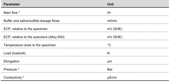
Table 2: Examples of parameters that were measured during the testing.
Parameter Unit
Main flow † l/h
Buffer and saline/sulfide dosage flows ml/min ECP, relative to the specimen mV (SHE) ECP, relative to the autoclave (Alloy 600) mV (SHE) Temperature close to the specimen °C
Load (loadcell) N
Elongation µm
Pressure ‡ Bar
Conductivity ‡ µS/cm
† Measured once a day.
‡ Measured value only for diagnostics, not used for evaluation.
Reference tensile testing procedure
A reference tensile test at 90°C was performed by Exova according to ASTM E21. The reference tensile testing was performed to acquire a material model for the material used, to base the FEM calculations on.
Material
The copper material used in the testing was supplied to Studsvik by The Swedish Radiation Safety Authority (SSM). The copper material was part of a canister lid (TX214 HT1,) which have been supplied to SSM from the Swedish Nuclear Fuel and Waste Management Co (SKB). The material was oxygen-free phosphorus-containing copper (Cu-OFP). Before delivery to Studsvik, it had un-derwent the heat treatment cycle HT1 (SKB name of procedure, which is representative of all SKB’s lids and bottoms). The chemical content of the material, as supplied by SKB, is given in Table 3.
The testing parameters are listed in Table 1. During testing, the load is continuously measured us-ing a load cell, and the elongation of the specimen is measured usus-ing a digital micrometer mounted on the load train outside of the autoclave. A certain amount of compliance will therefore exist in the stress-strain results obtained during the SSRT testing.
Figure 5: Schematic of the autoclave used for the experiments. Table 1: Summary of target testing parameters.
Parameter Target value
Temperature 90°C Cl- (as NaCl) 0.1 M S2- (as Na2S) Exposures 1 and 2 1·10-3 M Exposures 3 and 4 1·10-4 M Exposure 5 1·10-5 M Autoclave flow 1 l/h Strain rate† ~0.7·10-7 s-1 Maximum strain 9%
Testing time 2 weeks
† At the smallest section of the tapered gage section.
During the experiments, several parameters are measured and digitally logged once every minute to secure that the correct exposure environment is reached during the testing. Some, but not all, pa-rameters are listed in Table 2.
Table 2: Examples of parameters that were measured during the testing.
Parameter Unit
Main flow † l/h
Buffer and saline/sulfide dosage flows ml/min ECP, relative to the specimen mV (SHE) ECP, relative to the autoclave (Alloy 600) mV (SHE) Temperature close to the specimen °C
Load (loadcell) N
Elongation µm
Pressure ‡ Bar
Conductivity ‡ µS/cm
† Measured once a day.
‡ Measured value only for diagnostics, not used for evaluation.
Reference tensile testing procedure
A reference tensile test at 90°C was performed by Exova according to ASTM E21. The reference tensile testing was performed to acquire a material model for the material used, to base the FEM calculations on.
Material
The copper material used in the testing was supplied to Studsvik by The Swedish Radiation Safety Authority (SSM). The copper material was part of a canister lid (TX214 HT1,) which have been supplied to SSM from the Swedish Nuclear Fuel and Waste Management Co (SKB). The material was oxygen-free phosphorus-containing copper (Cu-OFP). Before delivery to Studsvik, it had un-derwent the heat treatment cycle HT1 (SKB name of procedure, which is representative of all SKB’s lids and bottoms). The chemical content of the material, as supplied by SKB, is given in Table 3.
Figure 6: Photograph of the TX214 HT1 Cu-OFP material used in the experiments. The black boxes and num-bers shows generally from where each specimen has been prepared.
Table 3: Chemical content (ppm unless given otherwise) of the Cu-OFP material used in the test.
Cu+P P Pb Bi As Sb Sn Zn Mn Cr Co Cd Fe Ni Ag Se Te S 99.99% 43-60 <1 <1 <1 <1 <0.5 <1 <0.5 <1 <1 <1 <1 2 12 <1 <1 6
Test environment
Na2S·9H2O (≥98%, Sigma Aldrich) and NaCl (≥99.5%, Sigma Aldrich) was used to simulate the
final repository environment. Na2HPO4·2H2O (≥98%, Sigma Aldrich) and NaH2PO4·2H2O (≥98%,
Sigma Aldrich) was used to maintain a pH of 7. NaOH (≥98%, Sigma Aldrich) and
Zn(CH3COO)2·2H2O (≥98%, Sigma Aldrich) was used to preserve water samples for analysis of
sulfide content.
1
2
3
4
5
6
7
8
9
10
SSRT Specimen manufacturing
Before the specimens could be produced, Finite Element Method (FEM) calculations were used to determine the specimen design and how to achieve the desired strain along the tapered gage sec-tion of the specimen, see Figure 7 and Figure 8.
Figure 7: Final drawing of the specimen design.
Figure 8: Illustration, based upon the FEM calculations, of the strain distribution axially along the tapered gage section of the specimen assuming a 1,500 μm elongation.
Note that originally, a maximum of 10% strain following a 1,500 μm elongation was planned for the experiments. The first experiment however resulted in a maximum ~9% strain following a 1,300 μm elongation (due to under estimation of compliance in the SSRT load train.). For easier comparison between the different experiments, the scope was changed to 9% strain following a
1,300 μm elongation for all experiments. The FEM calculations were re-evaluated to accommo-date for this.
Following the FEM calculations, the axial strain as a function of the distance to the narrowest part of the specimen gage section was calculated, see Figure 9. However, the FEM calculation used the un-deformed specimen as a frame of reference. For example, a point on the gage section that in the FEM simulation is shown to be 1 mm away from the narrowest part of the specimen, is on the real specimen measured to be 1 mm away from the narrowest part of the gage section plus the added strain over the 1 mm increment, added during testing. In order to change the frame of reference to the deformed specimen’s, the elongation was proportionally distributed across the specimen gage section according to calculated strain. The unmodified curve in Figure 9 thus shows the strain as a function of distance on the un-deformed specimen gage section while the modified curve show the strain as a function of distance on the deformed specimen. During evaluation the latter curve was used.
Figure 9: Unmodified (blur) and modified (orange) strain as a function of distance along the tapered gage sec-tion of the specimen, after applicasec-tion of 1,300 μm elongasec-tion.
A curve fit was used to estimate an equation for the strain as a function of distance from the nar-rowest part of the tapered gage section (shown in Figure 9), see Eq. 1.
𝑓𝑓(𝑋𝑋) = 𝐴𝐴 + 𝐵𝐵 ∙ 𝑋𝑋 + 𝐶𝐶 ∙ 𝑋𝑋2+ 𝐷𝐷 ∙ 𝑋𝑋3+ 𝐸𝐸 ∙ 𝑋𝑋4+ 𝐹𝐹 ∙ 𝑋𝑋5+ 𝐺𝐺 ∙ 𝑋𝑋6+ 𝐻𝐻 ∙ 𝑋𝑋7+ 𝐼𝐼 ∙ 𝑋𝑋8+ 𝐽𝐽 ∙ 𝑋𝑋9 (𝐸𝐸𝐸𝐸. 1) Where A = 8.78 % D = 4.30·10-2 % G = 8.45·10-6 % B = 0.764 % E = -1.31·10-3 % H = -2.99·10-7 % C = -0.401 % F = -8.27·10-5 % I = 4.99·10-9 % J = -3.27·10-11 %
Equation 1 was used to estimate the strain for any cracks that were observed in the material fol-lowing the experiments based upon the distance from the narrowest part of the tapered gage sec-tion to the observed crack.
A total of nine specimens were produced by Mikroverktyg AB according to the drawing in Figure 7 (a surplus of specimens was manufactured). All specimens had their major geometries checked either through a caliper or through a LOM, see Table 4.
All specimens gage sections were manufactured with a surface roughness of Ra 0.4.
Table 4: Specimen major geometries checked before experiments.
Specimen # Experiment # Specimen length † (mm)
Specimen main width ‡ (mm)
Tapered gage section width * (mm) 3 1 100.15 8.035 4.256 4 2 100.13 8.040 4.253 5 3 100.20 8.045 4.252 6 4 100.17 8.025 4.246 7 5 100.15 8.035 4.252
† Measured at Studsvik using a caliper. ‡ Measured at Mikroverktyg using a caliper.
* Measured at Studsvik using a LOM.
Exposures
Five sets of experiments were run. All experiments were run as expected with the following excep-tions:
Experiment one;
o The main flow and dosage flow rates were reduced for the last part of the experi-ment to conserve the dosage solutions to last the entire experiexperi-ment.
o The conductivity cell measuring the conductivity malfunction and showed a value several orders lower than expected.
Experiment two;
o The main flow and dosage flow rates were reduced for the last part of the experi-ment to conserve the dosage solutions to last the entire experiexperi-ment.
o The dosage flow of the sulfide/saline solution saw a momentary decreased flow rate most likely due to precipitation of NaCl. The sulfide/saline dosage rate was approximately 30% lower during ten hours of the experiment and 25% higher for four hours of the experiment.
Experiment three;
o The micrometer that measured the elongation malfunctioned towards the end of the experiment leading to a loss of elongation data. Once restored, the elongation measurement was reset, so the elongation data had to be manually adjusted.
Experiment four;
Experiment five;
o Due to malfunctioning equipment, no elongation data was recorded by the data logger for the initial 22 hours of the exposure. The lack of data does not affect the quality of the experiment nor the post-analysis.
o The loading of the specimen was unfortunately started somewhat pre-maturely, i.e. before the specimen had reached a stable ECP. However, only a minor part of the exposure was affected, and as such it is not expected that the result of the testing was influenced. Furthermore, the ECP of the autoclave was stable during the exposure and the analyzed sulfide concentration in line with the desired value. The exposure chemistry has thus been correct.
A summary of some of the experimental data measured during each of these experiments is shown in Table 5 below, and the full data for each experiment is shown in Appendix A–E, respectively for experiments 1 to 5.
Table 5: Average experimental data, and standard deviation, that were measured during the experiments.
Parameter Exp1 Exp2 Exp3 Exp4 Exp5
Sulfide (M) Start 0.8·10
-3 0.8·10-3 0.7·10-4 0.6·10-4 0.3·10-5 † End 0.9·10-3 0.9·10-3 0.6·10-4 0.6·10-4 0.3·10-5 † ECP, relative to the specimen (mV SHE) -736
±18 -637 ±2 -580 ±7 -575 ±14 -387 ±70
ECP, relative to the autoclave (mV SHE) -438
±15 -359 ±12 -294 ±6 -286 ±13 -210 ±10
Temperature close to the specimen (°C) 90.4
±0.2 90.2 ±0.1 90.2 ±0.2 90.1 ±0.2 90.1 ±0.2
Average Strain Rate (s-1)** 0.67·10-7 0.68·10-7 0.66·10-7 0.66·10-7 0.66·10-7
Pressure vs atm. (bar) ‡ 4.2
±0.1 4.0 ±0.1 4.2 ±0.1 4.1 ±0.1 4.2 ±0.1 Conductivity (μS/cm) ‡ N/A* 11,357 ±474 10,039 ±94 9,941 ±248 9,905 ±179
† The high saline concentration, meaning a high background matrix containing chloride ions used during the analysis, most likely meant a higher inaccuracy for the analyzed sulfide levels from Exp5.
‡ Only for diagnostic purposes.
* The conductivity during experiment 1 was too high for the conductivity cell to measure correctly. A new conductivity cell was used in the subsequent experiments.
** The average strain rate has been calculated for the narrowest part of the gage section.
Microscopy examinations
Upon completion of each experiment except specimen 7 originating from experiment 5, each spec-imen was cleaned in room-temperature concentrated HCl (Sigma-aldrich, puriss, ≥37%) using a nylon brush to remove any cupper sulfide on the surface. Following the cleaning, the surface of each specimen was inspected in either a LOM (Reichert Polyvar) and/or a Scanning Electrical Mi-croscope (SEM, JEOL JSM6300) for the presence of cracks. The specimens were then encapsu-lated in a resin epoxy and polished parallel along the specimen length to fabricate a cross section, see Figure 10.
The polishing procedure was done in the following steps:
1. Coarse grinding/felling using SiC-paper 220#/500#/1000# at 300 rpm.
2. Fine grinding using 9 µm diamond slurry on a Struers Resin Bond Diamond Grinding Wheel Allegro at 300 rpm.
3. Polishing using 9 µm diamond slurry on a Struers Polishing cloth DP-Dac at 150 rpm. 4. Oxide polishing using 0.04 µm colloidal silica suspension on a Struers Polishing cloth
OP-Chem at 150 rpm.
Care was taken throughout all examinations of this type to make sure that the polishing occurred at an angle and to a depth so that at least some (if any were observed) cracks on the surface would be revealed in the cross section.
Figure 10: Cleaning in HCl (top row) and polishing (bottom row) of an exposed copper specimen.
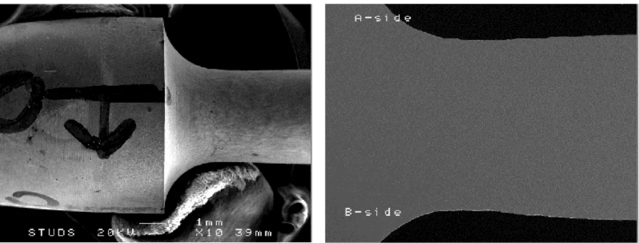
For each specimen, two sides having been examined corresponding to side A and B, see Figure 11, in a JEOL JSM6300 Scanning Electron Microscope (SEM).
Figure 11: Images of unpolished (left) and polished (right) Cu specimen depicting how side A and B have been defined.
Experiment five;
o Due to malfunctioning equipment, no elongation data was recorded by the data logger for the initial 22 hours of the exposure. The lack of data does not affect the quality of the experiment nor the post-analysis.
o The loading of the specimen was unfortunately started somewhat pre-maturely, i.e. before the specimen had reached a stable ECP. However, only a minor part of the exposure was affected, and as such it is not expected that the result of the testing was influenced. Furthermore, the ECP of the autoclave was stable during the exposure and the analyzed sulfide concentration in line with the desired value. The exposure chemistry has thus been correct.
A summary of some of the experimental data measured during each of these experiments is shown in Table 5 below, and the full data for each experiment is shown in Appendix A–E, respectively for experiments 1 to 5.
Table 5: Average experimental data, and standard deviation, that were measured during the experiments.
Parameter Exp1 Exp2 Exp3 Exp4 Exp5
Sulfide (M) Start 0.8·10
-3 0.8·10-3 0.7·10-4 0.6·10-4 0.3·10-5 † End 0.9·10-3 0.9·10-3 0.6·10-4 0.6·10-4 0.3·10-5 † ECP, relative to the specimen (mV SHE) -736
±18 -637 ±2 -580 ±7 -575 ±14 -387 ±70
ECP, relative to the autoclave (mV SHE) -438
±15 -359 ±12 -294 ±6 -286 ±13 -210 ±10
Temperature close to the specimen (°C) 90.4
±0.2 90.2 ±0.1 90.2 ±0.2 90.1 ±0.2 90.1 ±0.2
Average Strain Rate (s-1)** 0.67·10-7 0.68·10-7 0.66·10-7 0.66·10-7 0.66·10-7
Pressure vs atm. (bar) ‡ 4.2
±0.1 4.0 ±0.1 4.2 ±0.1 4.1 ±0.1 4.2 ±0.1 Conductivity (μS/cm) ‡ N/A* 11,357 ±474 10,039 ±94 9,941 ±248 9,905 ±179
† The high saline concentration, meaning a high background matrix containing chloride ions used during the analysis, most likely meant a higher inaccuracy for the analyzed sulfide levels from Exp5.
‡ Only for diagnostic purposes.
* The conductivity during experiment 1 was too high for the conductivity cell to measure correctly. A new conductivity cell was used in the subsequent experiments.
** The average strain rate has been calculated for the narrowest part of the gage section.
Microscopy examinations
Upon completion of each experiment except specimen 7 originating from experiment 5, each spec-imen was cleaned in room-temperature concentrated HCl (Sigma-aldrich, puriss, ≥37%) using a nylon brush to remove any cupper sulfide on the surface. Following the cleaning, the surface of each specimen was inspected in either a LOM (Reichert Polyvar) and/or a Scanning Electrical Mi-croscope (SEM, JEOL JSM6300) for the presence of cracks. The specimens were then encapsu-lated in a resin epoxy and polished parallel along the specimen length to fabricate a cross section, see Figure 10.
The polishing procedure was done in the following steps:
1. Coarse grinding/felling using SiC-paper 220#/500#/1000# at 300 rpm.
2. Fine grinding using 9 µm diamond slurry on a Struers Resin Bond Diamond Grinding Wheel Allegro at 300 rpm.
3. Polishing using 9 µm diamond slurry on a Struers Polishing cloth DP-Dac at 150 rpm. 4. Oxide polishing using 0.04 µm colloidal silica suspension on a Struers Polishing cloth
OP-Chem at 150 rpm.
Care was taken throughout all examinations of this type to make sure that the polishing occurred at an angle and to a depth so that at least some (if any were observed) cracks on the surface would be revealed in the cross section.
Figure 10: Cleaning in HCl (top row) and polishing (bottom row) of an exposed copper specimen.
For each specimen, two sides having been examined corresponding to side A and B, see Figure 11, in a JEOL JSM6300 Scanning Electron Microscope (SEM).
Figure 11: Images of unpolished (left) and polished (right) Cu specimen depicting how side A and B have been defined.
3. Results
Tensile testing
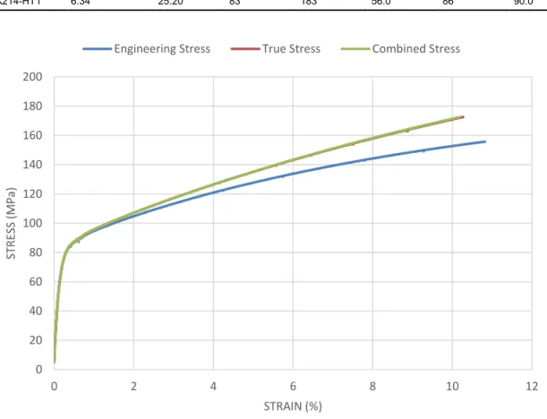
The results obtained from the tensile test performed by Exova at 90°C is shown in Table 6 and Figure 12. Note that Figure 12 only shows a part of the full Stress-Strain data acquired. True and combined stress both originate from the extensometer data below 25% strain, while the combined stress takes the cross-head displacement into account above this value. True and combined stress are thus identical in the interval shown in Figure 12.
Table 6: Results from the reference tensile testing.
Sample Diameter (mm) GL (mm) Rp0.20 (N/mm2) UTS (N/mm2)
%E1 %RA Temp (°C)
TX214-HT1 6.34 25.20 83 183 56.0 86 90.0
Figure 12: Engineering, true and combined stress vs strain from the tensile test performed at 90°C.
A curve fit was used to estimate an equation for the combined stress as a function of strain as shown in Figure 12, see Eq. 2.
𝑓𝑓(𝑋𝑋) = 𝐴𝐴 + 𝐵𝐵 ∙ 𝑋𝑋 + 𝐶𝐶 ∙ 𝑋𝑋2+ 𝐷𝐷 ∙ 𝑋𝑋3+ 𝐸𝐸 ∙ 𝑋𝑋4+ 𝐹𝐹 ∙ 𝑋𝑋5+ 𝐺𝐺 ∙ 𝑋𝑋6+ 𝐻𝐻 ∙ 𝑋𝑋7 +𝐼𝐼 ∙ 𝑋𝑋8 (𝐸𝐸𝐸𝐸. 2) Where A = 81.00355 D = 1.96103 G = -0.00878 B = 18.22726 E = -0.52234 H = 0.000481 C = -4.99723 F = 0.0874 I = -1.1E-05 0 20 40 60 80 100 120 140 160 180 200 0 2 4 6 8 10 12 ST RE SS ( M Pa ) STRAIN (%)
Engineering Stress True Stress Combined Stress
Equation 2 has later been used to estimate the stress for any observed crack (or crack-like defects) at a strain given by the FEM calculations bases upon measurements how far from the narrowest part of the tapered gage section that the crack was observed in the material following the experi-ments.
Slow Strain Rate Testing
Experiment one
After experiment one, specimen #3 was removed from the autoclave, see Figure 13. Prior to the post-exposure examination, the length and the width of the thinnest part of the tapered gage sec-tion were measured and compared with the pre-exposure data, see Table 7.
Figure 13: Photograph of specimen #3 after exposure one.
Table 7: Specimen major geometries checked pre- and post- exposure, and change.
Experiment # Specimen # Specimen length (mm) † Tapered gage section thickness (mm) ‡
Pre Post Change Pre Post Change
1 3 100.15 101.41 +1.26 4.256 3.858 -0.398
† Measured at Studsvik using a caliper. ‡ Measured at Studsvik using a LOM.
The post-exposure examination with stereo microscopy of the surface of the specimen from exper-iment one revealed several surface defects attributed to cracks, see Figure 14.
3. Results
Tensile testing
The results obtained from the tensile test performed by Exova at 90°C is shown in Table 6 and Figure 12. Note that Figure 12 only shows a part of the full Stress-Strain data acquired. True and combined stress both originate from the extensometer data below 25% strain, while the combined stress takes the cross-head displacement into account above this value. True and combined stress are thus identical in the interval shown in Figure 12.
Table 6: Results from the reference tensile testing.
Sample Diameter (mm) GL (mm) Rp0.20 (N/mm2) UTS (N/mm2)
%E1 %RA Temp (°C)
TX214-HT1 6.34 25.20 83 183 56.0 86 90.0
Figure 12: Engineering, true and combined stress vs strain from the tensile test performed at 90°C.
A curve fit was used to estimate an equation for the combined stress as a function of strain as shown in Figure 12, see Eq. 2.
𝑓𝑓(𝑋𝑋) = 𝐴𝐴 + 𝐵𝐵 ∙ 𝑋𝑋 + 𝐶𝐶 ∙ 𝑋𝑋2+ 𝐷𝐷 ∙ 𝑋𝑋3+ 𝐸𝐸 ∙ 𝑋𝑋4+ 𝐹𝐹 ∙ 𝑋𝑋5+ 𝐺𝐺 ∙ 𝑋𝑋6+ 𝐻𝐻 ∙ 𝑋𝑋7 +𝐼𝐼 ∙ 𝑋𝑋8 (𝐸𝐸𝐸𝐸. 2) Where A = 81.00355 D = 1.96103 G = -0.00878 B = 18.22726 E = -0.52234 H = 0.000481 C = -4.99723 F = 0.0874 I = -1.1E-05 0 20 40 60 80 100 120 140 160 180 200 0 2 4 6 8 10 12 ST RE SS ( M Pa ) STRAIN (%)
Engineering Stress True Stress Combined Stress
Equation 2 has later been used to estimate the stress for any observed crack (or crack-like defects) at a strain given by the FEM calculations bases upon measurements how far from the narrowest part of the tapered gage section that the crack was observed in the material following the experi-ments.
Slow Strain Rate Testing
Experiment one
After experiment one, specimen #3 was removed from the autoclave, see Figure 13. Prior to the post-exposure examination, the length and the width of the thinnest part of the tapered gage sec-tion were measured and compared with the pre-exposure data, see Table 7.
Figure 13: Photograph of specimen #3 after exposure one.
Table 7: Specimen major geometries checked pre- and post- exposure, and change.
Experiment # Specimen # Specimen length (mm) † Tapered gage section thickness (mm) ‡
Pre Post Change Pre Post Change
1 3 100.15 101.41 +1.26 4.256 3.858 -0.398
† Measured at Studsvik using a caliper. ‡ Measured at Studsvik using a LOM.
The post-exposure examination with stereo microscopy of the surface of the specimen from exper-iment one revealed several surface defects attributed to cracks, see Figure 14.
Figure 14: Selected SEM images of the specimen surface close to the narrowest part of the tapered gage sec-tion of the SSRT specimen exposed in experiment one.
The cross section analysis was performed in a SEM along both side A and side B. The distance from the narrowest part of the tapered gage section to any defects were measured, and the defects were visually analyzed to determine if they could be deemed to be a crack. Figure 15 and Figure 16 shows all defects observed for the specimen exposed in the first experiment that have been attributed to cracks. Additional defects, not positively attributed to cracks, are shown in Appendix F. A crack was in the evaluation defined as an observed surface defect, which had tended to grow preferentially to the surrounding material during the testing. The defects not at-tributed to cracks did not show such appearance, and analyzing these further was outside the scope of this work.
0 mm 2.26 mm
2.72 mm 4.34 mm
Figure 15: SEM images of the cracks observed and their distance to the narrowest part of tapered gage section on side A of the specimen cross section of the SSRT specimen exposed in experiment one.
0 mm 2.6 mm
Figure 16: SEM images of the cracks observed and their distance to the narrowest part of tapered gage section on side B of the specimen cross section of the SSRT specimen exposed in experiment one.
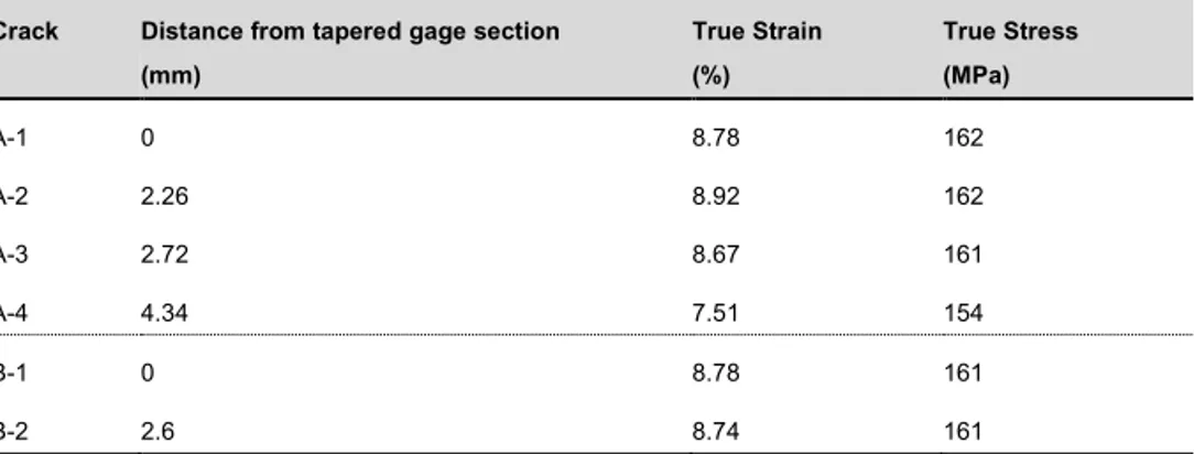
Equation 1 was used to estimate the true strain for which the crack had occurred, and Equation 2 was subsequently used to calculate the true stress that the strain corresponds to, see Table 8.
Figure 14: Selected SEM images of the specimen surface close to the narrowest part of the tapered gage sec-tion of the SSRT specimen exposed in experiment one.
The cross section analysis was performed in a SEM along both side A and side B. The distance from the narrowest part of the tapered gage section to any defects were measured, and the defects were visually analyzed to determine if they could be deemed to be a crack. Figure 15 and Figure 16 shows all defects observed for the specimen exposed in the first experiment that have been attributed to cracks. Additional defects, not positively attributed to cracks, are shown in Appendix F. A crack was in the evaluation defined as an observed surface defect, which had tended to grow preferentially to the surrounding material during the testing. The defects not at-tributed to cracks did not show such appearance, and analyzing these further was outside the scope of this work.
0 mm 2.26 mm
2.72 mm 4.34 mm
Figure 15: SEM images of the cracks observed and their distance to the narrowest part of tapered gage section on side A of the specimen cross section of the SSRT specimen exposed in experiment one.
0 mm 2.6 mm
Figure 16: SEM images of the cracks observed and their distance to the narrowest part of tapered gage section on side B of the specimen cross section of the SSRT specimen exposed in experiment one.
Equation 1 was used to estimate the true strain for which the crack had occurred, and Equation 2 was subsequently used to calculate the true stress that the strain corresponds to, see Table 8.
Table 8: Summary of results obtained from the SSRT testing during experiment one.
Crack Distance from tapered gage section (mm) True Strain (%) True Stress (MPa) A-1 0 8.78 162 A-2 2.26 8.92 162 A-3 2.72 8.67 161 A-4 4.34 7.51 154 B-1 0 8.78 161 B-2 2.6 8.74 161
Experiment two
After experiment two, specimen #4 was removed from the autoclave, see Figure 17. Prior to the post-exposure examination, the length and the width of the thinnest part of the tapered gage sec-tion were measured and compared with the pre-exposure data, see Table 9.
Figure 17: Photograph of specimen #4 after exposure two.
Table 9: Specimen major geometries checked pre- and post- exposure, and change.
Experiment # Specimen # Specimen length (mm) † Tapered gage section width (mm) ‡
Pre Post Change Pre Post Change
2 4 100.13 101.40 +1.27 4.253 3.905 -0.348
† Measured at Studsvik using a caliper. ‡ Measured at Studsvik using a LOM.
The post-exposure examination using microscopy of the surface of the specimen from experiment two revealed several surface defects attributed to cracks, see Figure 18.
Figure 18: Selected SEM images of the specimen surface close to the narrowest part of the tapered gage sec-tion of the SSRT specimen exposed in experiment two.
The cross section analysis was only performed in SEM along side B, which was thought to be rep-resentative for the specimen as a whole. The distance from the narrowest part of the tapered gage section to any defects were measured, and the defects were visually analyzed to determine if they could be deemed to be a crack. Figure 19 shows all defects observed for the specimen exposed in experiment two that have been attributed to cracks. Additional defects, not positively attributed to cracks, are shown in Appendix G.
0.6 mm 0.9 mm
Figure 19: SEM images of the cracks observed and their distance to the narrowest part of tapered gage section on side B of the specimen cross section of the SSRT specimen exposed in experiment two.
Equations 1 and 2 were used to estimate the true strain for which the crack had occurred, and to calculate the true stress that the strain corresponds to, see Table 10.
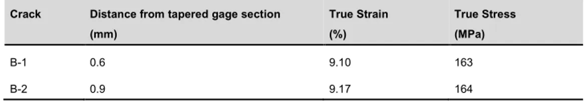
Table 10: Summary of results obtained from the SSRT testing during exposure two.
Crack Distance from tapered gage section (mm) True Strain (%) True Stress (MPa) B-1 0.6 9.10 163 B-2 0.9 9.17 164
Experiment three
After exposure three, specimen #5 was removed from the autoclave, see Figure 20. Prior to the post-exposure examination, the length and the width of the thinnest part of the tapered gage sec-tion were measured and compared with the pre-exposure data, see Table 11.
Figure 20: Photograph of specimen #5 after exposure three.
Table 11: Specimen major geometries pre- and post- exposure, and change.
Experiment # Specimen # Specimen length (mm) † Tapered gage section width (mm) ‡
Pre Post Change Pre Post Change
3 5 100.20 101.45 +1.25 4.252 3.869 -0.383
† Measured at Studsvik using a caliper. ‡ Measured at Studsvik using a LOM.
The post-exposure examination using microscopy of the surface of the specimen from exposure three revealed a very rough/coarse surface containing anomalies resembling craters, with very rough inner surfaces. Several defects could be seen when tilting the specimen inside the micro-scope, but none could positively be attributed to cracks. No microscopy images of the surface of the sample were collected from this post-exposure examination. During the polishing procedure, the specimen was tilted so that the polished surface would contain as many of these defects as pos-sible.
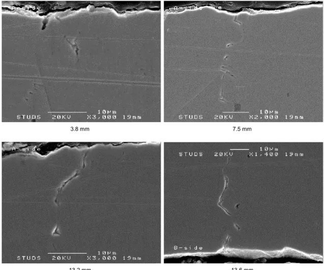
The cross section analysis was performed in an SEM along both sides of the specimen. For this specimen, no defects could positively be attribute as a crack, although several crack-like defects were observed. Figure 21 shows some examples of these defects, while Appendix H shows all de-fects observed for the specimen exposed in exposure three.
3.8 mm 7.5 mm
13.2 mm 13.6 mm
Figure 21: Example of SEM images of the defects observed and their distance to the narrowest part of tapered gage section on side A and B of the specimen cross section of the SSRT specimen #5 exposed in exposure three.
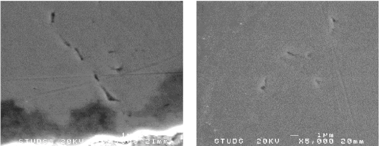
For comparison, additional regions were examined for similar crack-like defects on this specific specimen. Both the inner part of the specimen not directly exposed to the sulfide containing water, and the specimen head and full width gage section were examined for the presence of the surface defects (that were observed on the edges of the narrow gage section of the specimen). The purpose of this comparison was to look for similar defects in these regions. If any similar defects could be observed there as well, the defects most likely does not originate from the exposure to the sulfide containing water. The results are shown in Figure 22 for the inner section of the specimen, and in Figure 23 for the head and full width gage section, and they show that similar defects indeed could be located both inside the material, in the specimen head and in the full width gage section. It should however be noted that the amount of defects located inside the material, in the head and in the full width gage section was lower than what could be observed in the edges, but the defects could clearly be identified. The crack-like defects observed in the tapered gage section does thus most likely not originate from the exposure, and the origin of these defects have not been identi-fied and it is considered to be outside the scope of the current work. All defects, on the edges of the tapered gage section, inside the material and in the specimen head and full width gage section run vertically in the images, which corresponds to perpendicular to the axial length of the Cu spec-imen.
Table 10: Summary of results obtained from the SSRT testing during exposure two.
Crack Distance from tapered gage section (mm) True Strain (%) True Stress (MPa) B-1 0.6 9.10 163 B-2 0.9 9.17 164
Experiment three
After exposure three, specimen #5 was removed from the autoclave, see Figure 20. Prior to the post-exposure examination, the length and the width of the thinnest part of the tapered gage sec-tion were measured and compared with the pre-exposure data, see Table 11.
Figure 20: Photograph of specimen #5 after exposure three.
Table 11: Specimen major geometries pre- and post- exposure, and change.
Experiment # Specimen # Specimen length (mm) † Tapered gage section width (mm) ‡
Pre Post Change Pre Post Change
3 5 100.20 101.45 +1.25 4.252 3.869 -0.383
† Measured at Studsvik using a caliper. ‡ Measured at Studsvik using a LOM.
The post-exposure examination using microscopy of the surface of the specimen from exposure three revealed a very rough/coarse surface containing anomalies resembling craters, with very rough inner surfaces. Several defects could be seen when tilting the specimen inside the micro-scope, but none could positively be attributed to cracks. No microscopy images of the surface of the sample were collected from this post-exposure examination. During the polishing procedure, the specimen was tilted so that the polished surface would contain as many of these defects as pos-sible.
The cross section analysis was performed in an SEM along both sides of the specimen. For this specimen, no defects could positively be attribute as a crack, although several crack-like defects were observed. Figure 21 shows some examples of these defects, while Appendix H shows all de-fects observed for the specimen exposed in exposure three.
3.8 mm 7.5 mm
13.2 mm 13.6 mm
Figure 21: Example of SEM images of the defects observed and their distance to the narrowest part of tapered gage section on side A and B of the specimen cross section of the SSRT specimen #5 exposed in exposure three.
For comparison, additional regions were examined for similar crack-like defects on this specific specimen. Both the inner part of the specimen not directly exposed to the sulfide containing water, and the specimen head and full width gage section were examined for the presence of the surface defects (that were observed on the edges of the narrow gage section of the specimen). The purpose of this comparison was to look for similar defects in these regions. If any similar defects could be observed there as well, the defects most likely does not originate from the exposure to the sulfide containing water. The results are shown in Figure 22 for the inner section of the specimen, and in Figure 23 for the head and full width gage section, and they show that similar defects indeed could be located both inside the material, in the specimen head and in the full width gage section. It should however be noted that the amount of defects located inside the material, in the head and in the full width gage section was lower than what could be observed in the edges, but the defects could clearly be identified. The crack-like defects observed in the tapered gage section does thus most likely not originate from the exposure, and the origin of these defects have not been identi-fied and it is considered to be outside the scope of the current work. All defects, on the edges of the tapered gage section, inside the material and in the specimen head and full width gage section run vertically in the images, which corresponds to perpendicular to the axial length of the Cu spec-imen.