2012:37
Technical Note
Selective review of the hydrogeological
aspects of SR-Site
SSM perspektiv
BakgrundStrålsäkerhetsmyndigheten (SSM) granskar Svensk Kärnbränslehantering
AB:s (SKB) ansökningar enligt lagen (1984:3) om kärnteknisk verksamhet
om uppförande, innehav och drift av ett slutförvar för använt kärnbränsle
och av en inkapslingsanläggning. Som en del i granskningen ger SSM
konsulter uppdrag för att inhämta information i avgränsade frågor. I SSM:s
Technical note-serie rapporteras resultaten från dessa konsultuppdrag.
Projektets syfteSyftet med projektet är att ta fram synpunkter på SKB:s säkerhetsanalys
SR-Site för den långsiktiga strålsäkerheten hos det planerade
slutförva-ret i Forsmark. Synpunkterna ska baseras på en granskning av
huvudrap-porten för SR-Site. I granskningsuppdraget ingår att:
• belysa den övergripande kvaliteten på SKB:s redovisning,
• identifiera behov av kompletterande information från SKB och
• ta fram förslag på kritiska frågor som behöver granskas mer i detalj
i nästa fas av SSM:s tillståndsprövning.
Slutrapporten från konsultprojektet (denna Technical Note) är ett av
flera externa underlag som SSM kommer att beakta i sin egen granskning
av SKB:s säkerhetsredovisningar, tillsammans med andra
konsultrap-porter, remissvar från en nationell remiss och en internationell
expert-granskning av OECD:s kärnenergibyrå (NEA).
Författarens sammanfattning
Denna granskning av hydrogeologin är selektiv. Den fokuserar på
mät-ningar, tolkning och modellering av den potentiella förvarsvolymen, dvs.
sprickdomänen FFM01 på djup större än 400 m. Mätningarna och SKB:s
re-presentation av de mer transmissiva delarna av det hydrogeologiska systemet
accepteras som rimligt noggranna, i synnerhet på djup mindre än 150 m.
SKB beslutade att använda Posiva flödesloggen som huvudmetod för
fältmätningar. I denna granskning noteras metodens effektivitet och
snabbhet när det gäller att identifiera individuella flödande sprickor
eller flödesvägar. Betänkligheter framförs emellertid att
mätnoggrannhe-ten är för låg och att resultamätnoggrannhe-ten tekniken uppvisar vid låga flöden inte är
tillräckligt teoretiskt underbyggd.
SKB genomförde alternativa mätningar med ett så kallat rörgångssystem
(förkortat PSS; dvs. vatteninjektering i delar av borrhål som avgränsats
med manschetter) och fokuserade på mätningen av den hydrauliska
konduktiviteten. Det har endast lagts liten eller ingen vikt på att mäta den
oberoende ”kontrollerande” mätningen höjd vattenpelare. Därutöver har
PSS systemet givit en datasats som framträder som ”onaturlig” med en
signifikant ändring av uppvisat beteende precis under mätnoggrannheten.
SKB:s metod för att få fram parametervärdena från mätningarna i den
stokastiska diskreta spricknätverksmodelleringen (förkortat DFN) är svår
att förstå och olika aspekter av samma datasats används som indata och
DFN modellen anses i slutendan av en komplex modelleringsprocess ge
en bristfällig prediktion av förvarsvolymens flödesförhållanden. Vidare
anses att spricknätverksmodellen är nära perkolationsgränsen men att
den har för många flödande sprickor och att detta beror på antagandet
i den underliggande konceptuella modellen att sprickorna är lika breda
som långa. Det framförs ett alternativt koncept som adresserar dessa
tillkortakommanden.
Det bör framföras att tillvägagångssättet inom de hydrogeologiska
utred-ningarna i sprickigt berg generellt sett motsvarar disciplinens bästa
till-gängliga teknik. Det är olyckligt att det har lagts för lite tyngd på
potenti-ella förvarsvolymen som en signifikant del av säkerhetsanalysen bygger på.
ProjektinformationKontaktperson på SSM: Georg Lindgren
Diarienummer ramavtal: SSM2011-3640
Diarienummer avrop: SSM2011-4261
Aktivitetsnummer: 3030007-4015
SSM perspective
BackgroundThe Swedish Radiation Safety Authority (SSM) reviews the Swedish
Nu-clear Fuel Company’s (SKB) applications under the Act on NuNu-clear
Acti-vities (SFS 1984:3) for the construction and operation of a repository for
spent nuclear fuel and for an encapsulation facility. As part of the review,
SSM commissions consultants to carry out work in order to obtain
in-formation on specific issues. The results from the consultants’ tasks are
reported in SSM’s Technical Note series.
Objectives of the project
The objective of the project is to provide review comments on SKB’s
post-closure safety report, SR-Site, for the proposed repository at Forsmark.
The review comments shall be based on a review of the main report for
SR-Site. The review assignment comprises the following tasks:
• to evaluate the overall quality of SKB’s reporting
• to identify need for complementary information from SKB, and
• to propose critical issues that need to be addressed in more detail
in the next phase of SSM’s licensing review.
The final report from this consultant project (this Technical Note) is one
of several documents with external review comments that SSM will
consi-der in its own review of SKB’s safety reports, together with other
consul-tant reports, review comments from a national consultation, and an
inter-national peer review organized by OECD’s Nuclear Energy Agency (NEA).
Summary by the authorThis review of the hydrogeology is selective. It focuses on the measurement,
interpretation and modelling of the potential repository host rock, that is the
rock domain FFM01<-400m. It accepts as reasonably accurate the
measure-ment and representation of the more transmissive parts of the
hydrogeologi-cal system, particularly the near-surface 150m in the form presented by SKB.
SKB have decided that their main field measurement method is the Posiva
flow log. The review notes the speed and efficacy of the method in
iden-tifying individual actively flowing features/fractures. However, I have
concern that the lower measurement threshold is too high and behaviour
at low flows is insufficiently supported theoretically.
The subsidiary method based on the ‘Pipe String System’ (PSS) (i.e.
straddle packer injection testing) is strongly focussed on measuring
hydraulic conductivity. There is little or no emphasis on determining the
independent ‘checking’ measurement, head. In addition, the PSS method
has produced an ‘unnatural’ looking dataset with a significant change of
characteristic just below the measurement limit.
The method by which measurements produce parameters in the
probabi-listic ‘discrete fracture network’ (dfn) modelling is difficult to understand
and different aspects of the same dataset are used as input and
calibra-tion. There is a lack of sufficient independent checking methods.
At the end of the complex modelling process, the dfn model makes what
I consider a poor prediction of the flowing properties of the host rock. I
believe the dfn model is very close to its percolation threshold but has
too many active fractures. I believe this is caused by the assumption in
its underlying conceptual model of equi-dimensional hydraulically active
fractures.
I put forward an alternative concept that addresses these shortcomings.
It should be said that, overall, the approach to the hydrogeology of
fractu-red crystalline rock is current state-of-the-art. It is unfortunate that there
is insufficient focus on the host rock where a significant element of the
safety case resides.
Project information
2012:37
Author:
Selective review of the hydrogeological
aspects of SR-Site
John H. Black
Site Hydro, Nottingham, UK
This report was commissioned by the Swedish Radiation Safety Authority
(SSM). The conclusions and viewpoints presented in the report are those
of the author(s) and do not necessarily coincide with those of SSM.
Content
1. Introduction ... 3
1.1. Why a selective review ... 3
1.2. Approach to review ... 4
1.3. Layout of review ... 5
2. Field measurements relevant to the hydrogeology of FFM01 ... 6
2.1. What are the relevant measurements? ... 6
2.2. The Posiva flow logging measurements ... 6
2.3. The straddle packer (PSS) measurements ... 10
3. The conceptual model and its numerical implementation ... 12
3.1. The discrete fracture approach ... 12
3.2. SKB’s hydrogeological concept ... 12
3.3. An alternative conceptual model ... 16
3.3.1. A structural model as underpinning ... 16
3.3.2. The behaviour of systems of non-equi-dimensional fractures ... 17
3.3.3. The alternative models project undertaken by SKB ... 21
3.4. Summary of conceptual and numerical modelling ... 22
4. Checking measurements ... 22
4.1. Introduction ... 22
4.2. Heads from the straddle-packer testing ... 24
4.2.1. Extracting values of head from the PSS testing ... 24
4.2.2. Converting pressure to environmental head ... 24
4.2.3. Environmental heads in the KFM boreholes ... 25
4.2.4. Causes of head variations at depth ... 28
4.3. Heads in the modelling ... 29
5. The hydrogeology of EDZs ... 30
6. Discussion and conclusions ... 30
7. Non SR-Site references ... 31
Appendix 1 ... 32
Coverage of SKB reports ... 32
Appendix 2 ... 33
Suggested needs for complementary information from SKB ... 33
1. Transfer of head boundary conditions ... 33
2. Values of bulk K for FFM01 below 400m depth ... 33
3. Theoretical assessment of the Posiva flow logging method in non-ideal conditions ... 33
Appendix 3 ... 35
Suggested review topics for SSM ... 35
1. Sparse channel networks near the percolation limit ... 35
2. Distance to chokes and other borehole test assumptions ... 35
3. Head variability and monitoring strategy ... 36
4. Consolidation and dilation ... 36
5. The Excavation Damaged Zone ... 36
1. Introduction
1.1. Why a selective review
The documentation comprising the SR-Site Project is voluminous and aspects of hydrogeology form a significant element. It would be unreasonable to attempt a comprehensive critique of all hydrogeological aspects within the relatively short time available. I have therefore decided to review only those elements that could have a significant impact on the outcome of the Safety Case for a repository at Forsmark.
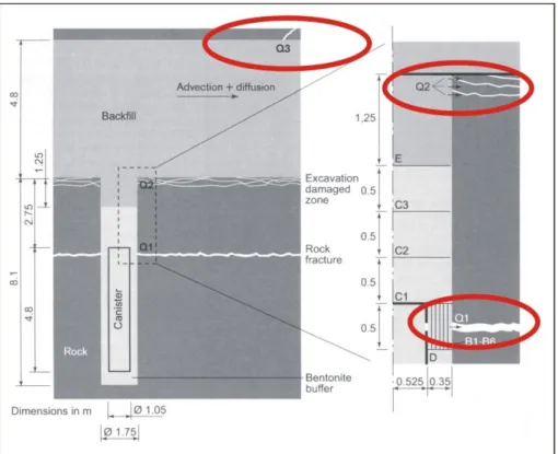
To the best of my knowledge, the Safety Case gains negligible potential benefit from advective transport within the near-surface groundwater system or the so-called ‘deformation zones’, both of which are considered to be highly transmissive. Since the evaluation of the more permeable near-surface plus the ‘deformation zones’ is relatively standard hydrogeology and the parameter values derived by SKB appear reasonable, I am assuming that SKB’s interpretation is adequately accurate. Hence, I am not considering SKB’s documentation on these subjects in this review. Essentially, ignoring the hydrogeology of the deformation zones means ignoring the ‘far-field’. Thus this review concerns groundwater flow and nuclide transport in the ‘near-field’, broadly described as ‘averagely fractured bedrock’. In the terminology of the Safety Case, I am reviewing the understanding and parameterization of ‘transport paths’ Q1, Q2 and Q3 (see Figure 13-13 of TR-11-01 reproduced here as Figure 1).
Figure 1. Annotated summary of Fig 13-13 of TR-11-01 showing potential transport
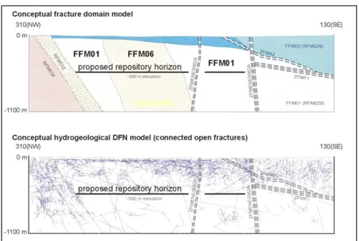
SKB have adopted an overall geological and hydrogeological concept whereby crystalline bedrock is categorised as either ‘fracture zones’ (termed ‘Hydraulic Conductor Domains’ at Forsmark [Figure 3-2 in R-09-22]) or background rock (termed ‘Hydraulic Rock mass Domains’ in R-09-22). I do not disagree with this approach though I have not examined how it is applied to the rock at Forsmark (i.e. in terms of extensiveness or local scale fracture density). They have further sub-divided the ‘Hydraulic Rock mass Domains’ into 6 sub-volumes termed ‘fracture domains’ based on their fracture characteristics. The repository is proposed to be excavated within ‘fracture domains’ FFM01 and FFM06, the configuration of which relative to the proposed repository is shown in Figure 2 (based on Figure 4.23 of TR-11-01 Pt 1).
This review therefore concerns the fracture domains FFM01 and FFM06, their conceptualisation, parameterisation and measurement in the field.
Figure 2. Proposed location of the repository within ‘fracture domains’ FFM01 and
FFM06 (slightly modified Figure 4.23 from TR-11-01 Part 1)
1.2. Approach to review
Although SKB have published work of this type before in SR-Can, it should be borne in mind that basing a major proportion of their field measurements on differential flow logging and interpreting via ‘discrete fracture network’ (dfn) models is an innovative approach in the field of ‘hard-rock’ hydrogeology. This means there are few precedents on which to base this review. Whilst at first sight, it might seem quickest to start with the Safety Case outcomes and work back through the underlying premises checking their validity, this approach does not readily lend itself to the consideration of alternative concepts or interpretations. One of the main problems is the probabilistic modelling method which does not lend itself to perceiving ‘cause-and-effect’.
Instead, I have followed the alternative method of starting with the field
measurements and working forwards through SKB’s stream of logic attempting to identify alternative concepts or interpretations where appropriate.
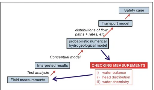
Figure 3. The logic stream of hydrogeological results and interpretation within the
SR-Site Safety Case
In common with any groundwater investigation using modelling, there is a need to obtain additional independent measurements in order to be able to check that the modelling produces outcomes that accord with reality. These ‘checking
measurements’ are usually a major help in demonstrating that the groundwater system is understood adequately well. They are also included in this review of the hydrogeology of Forsmark’s fracture domains FFM01 and FFM06 (N.B. There is little difference hydraulically between FFM01 and FFM06 so I only refer to FFM01 in the text below.)
1.3. Layout of review
The review is laid out in the following order which is not in order of importance: 1. Field measurements and their interpretation, particularly the Posiva Flow
Log and the straddle packer injection testing.
2. The adoption of a specific conceptual model and its numerical equivalents. 3. Independent ‘checking measurements’.
I have also included a brief section on the hydrogeology of the Excavation Damaged Zone.
2. Field measurements relevant to the
hydrogeology of FFM01
2.1. What are the relevant measurements?
There are effectively only two measurement methods that are relevant to groundwater flow in the background rock (I am using this term to refer to the fractured rock termed ‘fracture domain FFM01’ [and FFM06].) They are the single-borehole, straddle packer injection tests using the ‘PSS’ (pipe string system) equipment and the single-borehole ‘difference flow-logging’ using the Posiva originating equipment. The multi-borehole pumping tests that were performed are only really relevant to the behaviour of the near-surface system and the major deformation zones. The single point dilution tests were not performed in sufficient numbers to influence the parameterisation of the background rock.
2.2. The Posiva flow logging measurements
Together with the discrete fracture network (dfn) approach to modelling, the Posiva flow logging (PFL-f) method lies at the heart of SKB’s approach to the
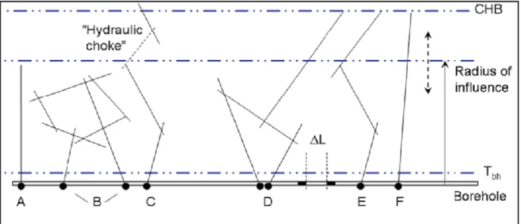
hydrogeology of a repository in crystalline bedrock. This is because it purports to measure transmissive features intersecting the borehole down to a spatial definition of 0.1m. Essentially, the method aims to measure the transmissivity of individual fractures intersected by any exploratory borehole. However, in order to be recorded, fractures have to exceed a value of transmissivity at the borehole of at least 1 x10⁻⁹ m2/s [page 38, R-07-48]. In addition to this ‘at-borehole’ criterion, the use of a week-long period of pumping prior to measurement means that all candidate fractures must not be connected to the ‘far-field’ (i.e. within the radius of influence of the pumping) by a controlling fracture (i.e. a ‘hydraulic choke’) with a value below the measurement threshold. This concept is repeated regularly throughout SKB’s documentation and is illustrated in Figure 4 (figure taken from page 332, TR-10-52, caption by this author)
Figure 4. The configurations of fractures that would yield an identified inflow using the
PFL-f method. Inflow points A and B are never recorded and C only if the ‘hydraulic choke’ allows sufficient flow at C that it exceeds a T value >1 x 10⁻⁹ m2/s. Inflow points D, E and F
require a ‘hinterland’ of fractures allowing the same. (CHB = constant head boundary, ΔL = interval length = 0.1 m)
At first sight, the lower measurement limit of a flow rate equivalent to a
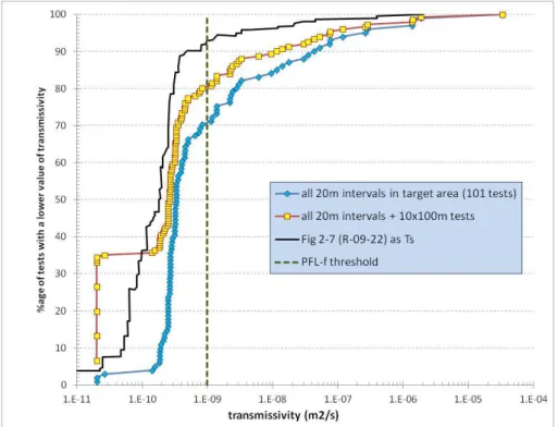
transmissivity value of 1 x 10⁻⁹ m2/s might seem small, but it should be viewed in relation to the dataset of more conventional straddle packer tests derived by the site characterisation project. The comparison is illustrated in a slightly odd way by Selroos and Follin (R-09-22) in their Figure 2-7 where they plot the cumulative distribution of 151 twenty metre long straddle packer tests from below -400m in the ‘target volume’ at Forsmark. It is odd in that the x-axis is hydraulic conductivity (rather than transmissivity) and the lower measurement limit of the PFL-f method is omitted.
I have replotted Figure 2-7 in terms of transmissivity (see Figure 5 which is based on digitising Figure 2-7) but encountered several problems. Firstly, I could only find 101 twenty-metre PSS tests in the target volume below 400m depth (based on the ‘Sicada’ tables appended to each borehole PSS report), not 151 as reported by Selroos and Follin. This set is plotted in Figure 5. If I assume that the extra 50 twenty-metre tests are actually 10 hundred-metre tests all at the lowest value of transmissivity reported for twenty-metre tests, I derive the modified data set of Figure 5.
I conclude that the origin of the dataset in Figure 2-7 is unclear. It probably includes an assumption about dividing transmissivity values for hundred-metre tests into five equal parts. It probably also involves assigning some of the higher values to ‘deformation zones’ and excluding them from consideration within the context of [hydraulic] ‘fracture domains’. There is an error in Table 2-1 (R-09-22) since I could find no record of PSS measurements in KFM01B or KFM02B.
Figure 5. The value of the PFL-f lower measurement limit viewed relative to transmissivity values measured by the straddle packer method below -400m in the target volume at Forsmark. The ‘all 20m intervals’ dataset is derived from tests in KFM boreholes 1D, 2A, 4A, 5A, 6A, 6C, 8A, 8C and 9B.
The most obvious conclusion to be drawn from Figure 5 is that the measurement limit for the PFL-f method excludes results from at least 70% and possibly 90% of the ‘background rock’. Also, roughly 60% of the fractured rock has an average hydraulic conductivity in the single decade of values just below. This is in contrast to parameter space above the measurement limit where 10% of values occupy three decades. The implication of this is that 90% of the ‘background rock’ goes unmeasured by the hydraulic measurement method upon which the hydraulic parameterisation of the geological ‘dfn’ model is based.
Returning to the PFL-f method itself, it is basically a highly refined flow logging method: an approach that has been previously used more qualitatively in
groundwater abstraction for many decades. It contains several innovations. It uses a highly sensitive heat pulse flow meter within a small-diameter guide tube which ‘concentrates’ the flow. It includes a highly sensitive pressure transducer within the test zone in order to know the absolute pressure immediately adjacent to the inflow point. Lastly, it includes two sets of rubber discs to define the test zone and a by-pass tube to allow flow within the rest of the borehole to remain ‘undisturbed’ by the isolation of the test zone. Although the system is supposed to have the same head inside the disc-defined test zone as outside it, the main requirement to enable the use of the PFL-f method is a smooth, preferably core-drilled, borehole. However, this smoothness requirement tends to break down where the borehole intercepts open fractures.
The main operational concept of the machine is that test zone flow is guided through a small diameter tube and whole borehole flow is guided through a large diameter tube. Since head loss through a tube is related to tube diameter and flow rate, the choice of tube diameters determines the head differences between the test interval and the upper and lower sections of borehole. These head differences occur across the rubber discs which do not seal the test interval like an inflated packer. Since the rest of borehole flow and the individual fracture flows vary throughout the borehole, flow leakage across the discs must vary both in direction and magnitude.
I have read both Ludvigson et al., (R-01-52) and Öhberg and Rouhiainen, 2000 and find no theoretical consideration of these effects. I wonder what factors were used to determine the most appropriate diameters of the flow-through tubes. Indeed, all assessments of the effectiveness or correctness of the PFL-f method seems to be based on comparing results to straddle packer tests.
The most extensive set of comparisons between PFL-f and PSS data is contained in Follin et al., (Sections 4.3 & 4.5of R-07-48) where (almost) all KFM boreholes between 1 and 8 where both methods have been used are cross-plotted. I include copies of three (KFM6A, 4A and 8A) in Figure 6. They are re-plotted in order to include a trend line and improve clarity. Each of them shows roughly similar behaviour of increasing divergence as transmissivity decreases with the PFL-f method recording the lower value.
The other notable feature of the plots is the number of straddle packer measured flowing intervals that are not seen by the PFL-f method (values are placed to the left of the Y-axis at an arbitrary value of PFL-f transmissivity). Values from KFM04A are particularly noteworthy because some ‘high’ values of PSS transmissivity are not ‘seen’ by the flow logging method. However it should be borne in mind that there are only 3 twenty metre tests and 4 five metre tests below -400m elevation in FFM01 in borehole KFM04A. In other words, most of these considerations do not concern ‘background rock’ in the repository zone.
Figure 6a
Figure 6b
Figure 6c
Follin et al., (R-07-48) explain the ‘decrease-with value’ discrepancy on the grounds that the straddle packer testing is short term and the flow logging is long term. They explain the ‘unseen anomalies’ in terms of a short term value that declines with time to a value less than the flow-logging threshold. This is the idea of ‘hydraulic chokes’ that is introduced here in Figure 4.
I am sceptical of this argument because the decline of inflow with time should be proportional to transmissivity so all inflows of the same value should be affected equally. On the other hand, the ‘decrease-with-value’ deviation seems to lead to greater spread with decreasing transmissivity. As far as the choke explanation is concerned, KFM04A exhibits a three decade spread of ‘unseen anomalies’. The upper values could not be expected to decline gradually to less than the threshold and a ‘barrier boundary’ would need to act rather suddenly. Also high
transmissivity means a large region of influence of a test so the immediate fracture cluster (compartment) would have to have large physical dimensions.
In summary, the PFL-f method is innovative and throws up a considerable number of questions. The relatively high threshold means that it does not identify many flowing fractures in the repository host rock region. I am concerned by the lack of theoretical or numerical background to:
1. The conceptual basis of the PFL-f method (for instance, in a practical test how much is the local fracture flow system disturbed by the presence of the flow tube and discs and the difference in head across the bypass tube?) 2. The idea of ‘hydraulic chokes’ (If they are inherent in nature, are they in
the numerical modelling? What sort of distances and scales are involved? If they occur every 10 metres or more then transport pathways Q1 and Q2 could occur within a ‘compartment’ and the censoring by flow-logging is not conservative.)
2.3. The straddle packer (PSS) measurements
The straddle packer measurements using the ‘Pipe String System (PSS) are entirely conventional and have been gradually developed over the last 40years. The approach involves a short period of water injection at constant head, followed by shut-in and a short period of recovery (usually not complete recovery).
The lower measurement limit of the method is determined by the lower
measurement limit of the flow meter and the stability (or otherwise) of the pressure in the test zone following isolation by packer inflation. It is claimed to be similar to the PFL-f method at 8 x 10⁻¹⁰ m2/s (Selroos and Follin, page 21, R-09-22). Like the PFL-f method this is a relatively high value given the nature of the ‘background rock’ in the region of the repository.
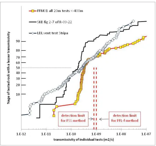
After much testing in fractured crystalline bedrock, I have come to expect test results for hydraulic conductivity (or transmissivity for tests of uniform interval length) to adhere to a broadly lognormal distribution. This is most easily recognised as a straight line form on a plot using equal axis length for each standard deviation either side of a median value. I have therefore plotted the twenty metre PSS results from Figure 2-7 of R-09-22 in the log normal form in Figure 7 together with the basic set of actual <-400m FFM01 twenty metre tests from SICADA. I have also included 140 tests of about 2m length from around the LBL ventilation test at 340 m depth in the Stripa Mine (measured in 1979!). The straight-line form of the Stripa
tests is clearly evident though it should be remembered that since the interval length is a tenth of the Forsmark data, the Forsmark datasets would be displaced leftwards by an order of magnitude if the X-axis was the logarithm of hydraulic conductivity. Notwithstanding the relative values of hydraulic conductivity, the profiles from Forsmark do not look natural. They could be interpreted as bi-modal but the less conductive portion is too permeable to be un-fractured matrix bedrock. In my judgement the Forsmark distributions appear to be strongly affected by the lower measurement limit of the test method.
Figure 7 Comparison of PSS twenty metre tests with some two metre tests from
Stripa, all plotted using a normalised Y axis.
When examining the testing reports, I discovered quite a few discrepancies that made their interpretation more difficult than necessary and indicated that field practice had not followed that indicated in the text of the reports. In particular, I found that:
1. The arrangement of the equipment did not match diagram 4-2 in 17 of the 21 tests and the co-ordinate system was misinterpreted by the authors of the reports.
2. The head of water above the packers was not measured by a transducer within the string as illustrated but in the open hole near the surface in over half of the tests.
3. The transducer inputs got misidentified in boreholes KFM11A and 12A. The testing used test interpretation software of current state-of-the-art slightly adapted from its water resources origins. It assumes space-filling, integer-only, flow configurations with the emphasis on 2D radial flow. When faced with 1D flow it
infers an axis parallel planar fracture rather than a channel. These assumptions have an impact on any calculation of ‘distance to a boundary’ which is considered to be an important issue in understanding the behaviour of ‘background rock’ under test. I note that most of the interpretations calculate a value for skin factor and that 80% of the tests derive a negative value. This implies that in the immediate vicinity of the borehole, head does not decline with distance at a rate indicative of cylindrical flow. It declines less quickly than expected. This implies linear rather than spherical flow. In other words, I would interpret the occurrence of negative skin factors in 80% of the test analyses to indicate that the borehole is predominantly connected to channels.
3. The conceptual model and its numerical
implementation
3.1. The discrete fracture approach
The discrete fracture approach adopted by SKB is based on the idea of calculating flows through discrete fractures in order to obtain an accurate estimate of overall groundwater movement, nuclide transport within that flow and natural
representation of dispersion. The basic geometry of the numerical groundwater model is a structural model. To calculate groundwater flow, the fractures, arranged according to the geometry of the geological structure, are assigned values of
transmissivity according to a probability distribution and the outcomes are compared to measurements in boreholes. Within this process the fracture density is thinned from considering every fracture (closed and open) for the structural model to a series of subsets of active connected fractures.
Apart from some identified structures (the deformation zones), the numerical representation of the structural model is probabilistic. In other words, the vast majority of fractures are not individually identified and are placed in the model according to some rules. In order to obtain ‘average’ behaviour from a model of this type, multiple realisations need to be undertaken and averages derived from the sum of the results.
The approach, with its multiple rules, intricate procedures and probabilistic method makes it difficult to follow and even more difficult to check without using a similar tool. However, the modelling process is addressed in a specialist review by a fellow reviewer with access to such a model.
In the review here, I examine some of the assumptions of the concept, some of the rules within the modelling process and some of the possibly diagnostic outcomes.
3.2. SKB’s hydrogeological concept
The hydrogeological concept is pictorially summarised in Figure 3-2 of Selroos and Follin (R-09-22) (reproduced below). The geometry of the soil zone is designated
and the location, orientation and extent of the hydraulic conductor domains is determined from geological mapping, boreholes and geophysical investigations. The rest of the system comprises ‘hydraulic rock mass domains’ (HCD) which are assigned fracture (geometrical) characteristics also by structural interpretation. Thus essentially the major features are identified geologically and are assumed to be hydrogeologically different from the rest of the rock mass. There is an implicit assumption that the HCDs are more transmissive than the rest of the system but I believe the hydraulic measurements form a single rather than bi-modal distribution.
The second sub-division is into different rock domains, the repository being located within FFM01 (see Figure 2). Within the modelling process reported in Follin et al., R0748, FFM01 is further subdivided into 3 hydrogeological units by depth, -above -200m, -200m→-400m and -400m→depth.
It should be borne in mind that the interpretation within the structural analysis defines the orientations of the fracture sets, the density of fractures within each set and their distribution of sizes. This is mainly based on mapping exposures at surface and the density and size interpretations are based on the assumption that the observed fractures are equi-dimensional (i.e. discs, or near circular polygons). Mapping indicates a power law relationship between fracture trace length and frequency of occurrence (i.e density) and using the equi-dimensional assumption this is extended to a power law relationship between fracture density (expressed as area per unit volume, P32) and fracture extensiveness (expressed as an equivalent radius, r).
The next stage of attaching hydraulic parameters to the fractures is more
problematic. It is obvious, based on even the most cursory examination, that most mappable fractures are not at all transmissive and therefore that the ultimate hydrogeological ‘discrete fracture network’ (dfn) model should be a ‘thinned-out’ version of the geological dfn model. Follin et al., (R-07-48) identify four types of fracture,
Sealed (as observed in core material).
Open (observed as a natural break in core material)
Partly open (observed as a partial natural break in core material) PFL anomaly (open fractures associated with flow into/out of a borehole
during flow logging)
They subsequently combine ‘open’ and ‘partly open’. The next important assumption (Follin et al, R-07-48 page 158) is that:
“open fractures form potential conduits for groundwater flow, whether they actually provide paths for flow depending on their connectivity and
transmissivity. The PFL-anomaly fractures represent a sub-set of the open fractures that are both connected to a wider network and have a
transmissivity above a threshold which will give flow measurable by the PFL-f method.”
So, the ‘open’ fractures form the basis of the hydrogeological dfn model. However, although the fracture orientation parameters of the geological dfn model are retained in the hydrogeological dfn, the size-density relationship is not. Note from Follin et al., R-07-48 page 158:
“…..we are interested in the fracture size distribution of only those fractures that contribute to the hydrogeological system, i.e. open fractures and PFL-anomaly fractures. Clearly this will be a sub-set of all fractures, but the parameter distributions of this sub-set do not necessarily bare a simple relationship to those for all fractures derived in Geo-DFN models.”
It would seem that the size-density relationship is adjusted to fit the frequency of very large features (lineaments) mapped on the surface and open fractures logged in core, all within the bounds set by the relationship involving all fractures both open and closed. The outcome of this process in terms of an ‘open fracture’ dfn model is provided in many reports, the extracted version below being from SKB TR-10-52, page 337. I have modified it to exclude the two higher elevation layers of FFM01 and include a ‘total’ for the area per volume intensity, P32. It should be noted that the classic work of Robinson, 1984 identified that equal-sized, square fractures, orientated orthogonally but randomly located , had a percolation threshold of 0.19 (in terms of number of fractures per unit volume). Bearing in mind that the fractures in SKB’s model are approximately circular, a unit radius fracture has an area of , so the percolation threshold should have a P32 value of 0.6 m-1 (i.e 0.19 x π). This means that SKB have chosen a set of densities such that the system only just percolates.
As far as I can tell, the fracture sizes included in the model range from r0 (=0.038m
[the borehole radius]) up to 564m (the radius of a 1km2 circle).
Up to this point the fractures in the hydrogeological dfn model have no values of transmissivity assigned to them. This appears to be achieved by a trial-and-error method using three different size-transmissivity correlation models (see Table 6-74 of TR-10-52): correlated, semi-correlated and uncorrelated. I do not know from whence they derive their transmissivity distribution unless it is the set of PFL-f values. SKB then compare the outcomes from 10 realisations of their three correlation models via the mechanism of an imaginary investigation borehole against four statistics derived from borehole measurements. They are listed on page 329 of TR-10-52:
1. Average total flow rate to the simulated abstraction borehole over ten realisations.
2. Histogram of log(Q/Δh) to the simulated abstraction borehole as an average over ten realisations.
3. Bar and whisker plot of minimum, mean minus standard deviation, mean, mean plus standard deviation, maximum of log(Q/Δh) to the simulated abstraction borehole within each fracture set taken over all realisations.
4. The average numbers of flowing fractures within each fracture set giving specific capacities to the simulated abstraction borehole above the measurement limit of the PFL method.
The outcome of this process for the ‘background rock’ in the repository zone for the first statistic, average ‘specific capacity’ is given in Table 11-21 as:
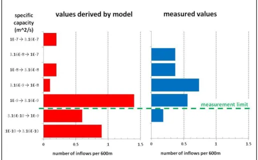
Measured PFL-f data 3.8x10⁻⁸ m2/s Model using semi-correlated T – size relation 5.4 x10⁻⁸ m2/s Model using correlated T – size relation 5.4 x10⁻⁸ m2/s Model using uncorrelated T – size relation 0.8 x10⁻⁸ m2/s Based on this outcome, SKB decided that their preference was to use the semi-correlated relationship but that it didn’t matter much either way. Their result for the second statistic was considerably less convincing. I have re-plotted Figure 11-15 of Follin et al, R-07-48 for the sake of clarity and to insert the lower measurement limit of the PFL-f method.
Figure 8 Comparison of measured and modelled values of number and magnitude of
inflows. (based on Figure 11-15 of R-07-48)
The third statistic is used to identify that only the NE and horizontal fracture sets provide measured inflows and that only the N-S and horizontal fractures provide inflows in the dfn model.
The authors do not mention the fourth statistic again.
My view of these outcomes is that the results in Figure 8 are poor. Whilst I acknowledge that the lower measurement limit is, for practical reasons, slightly variable, I do not believe that the average of 10 realisations should produce almost half of the outcomes below the field measurement limit and a further 40% at the measurement limit. Also, the modelled results appear rather ‘lumpy’ whereas the measured results look like a relatively smooth distribution. In general, I would have
thought that there are so many intermediate rules and relationships within the dfn process that can be used to ‘drive’ the outcomes that I would have expected a better match than illustrated in Figure 8.
My guess concerning Figure 8 is that although it is very close to the percolation threshold, it is still an overly dense network with too many connected fractures intercepted by the imaginary borehole. The final network is largely matched on total inflow so the excessive number of inflow points require to be apportioned negligible values of transmissivity in order to meet the total inflow criterion.
I find the dfn approach generally disconcerting because it is difficult to gain a ‘rough estimate’ of the large-scale value of hydraulic conductivity. Is the potential hostrock in the 1 x 10⁻⁹, 1 x 10⁻¹⁰ or 1 x 10-11 m/s general range? To some extent, SKB have provided parameter values within Figures 6-64 and 6-65 (of TR-10-52) that enable bulk permeability to be estimated. Figure 6-65 yields an average value of the frequency of open connected fractures (i.e ‘PFL’ fractures) within the lower part of FFM01 at 5 per kilometre or 0.005 m-1. Similarly, Figure 6-66 shows a geometric mean for the specific capacity of ‘flowing’ fractures as 6.5x10⁻⁹ m2/s. Elsewhere, on page 332 of TR-10-52, the Thiem equation is used to equate values of specific capacity directly with those of transmissivity. Thus, a 200m thickness of rock containing one open fracture with a value of transmissivity of 6.5x10⁻⁹ m2/s becomes a block with an average hydraulic conductivity of 3.25x10⁻¹¹m/s. This is low as a large-scale average.
However, another entry on Figure 6.64 (of TR-10-52) shows the average frequency of ‘open’ fractures in the lower part of FFM01 as 615 per kilometre (or 0.615 m-1). Bearing in mind that the hydrogeological dfn model assumes that all ‘open’ fractures are transmissive, 0.615 would thus be the fracture frequency associated with it. Since the hydrogeological dfn model has a P32 of 0.629 and the PFL fractures are 123 times less frequent (i.e. 0.615/0.005) then the P32 of the PFL fractures works out at 0.005. By a large margin, this is not a high enough density to percolate.
Lastly, Table 6-78 suggests large-scale values of hydraulic conductivity to apply to bedrock outside the target area but at similar depth at 3x10⁻⁹ m/s. A target area value of large scale hydraulic conductivity that is 100 times less permeable than the adjacent rock seems highly unlikely.
3.3. An alternative conceptual model
3.3.1. A structural model as underpinning
The SKB approach places much emphasis on geological investigation of the potential site and the structural model that underpins the hydrogeological interpretation is a natural consequence. However, turning two-dimensional maps and one-dimensional logs into a three-dimensional construct requires some key assumptions. In the case of fractures and fracturing, it requires the interpreter to assume some shape (i.e. square, circular, rectangular, elliptical, etc) for every observed fracture in order to derive values for fracture density and fracture size (extensiveness) in three dimensions. Any assumption other than equi-dimensional (i.e. squares, circles or ‘simple polygons’) gives rise to huge complexity and even
more subsidiary assumptions. However, the equi-dimensional assumption has been used in structural geology for many decades without widespread problems arising. At first thought, it seems perfectly logical to use a structural model to underpin a hydrogeological model and the procedure lies at the heart of all practical numerical groundwater modelling. But is it logical when applied to groundwater flow through fractures in crystalline rock? Flow through rough fractures has long been recognised as occurring in channels, effectively one-dimensional pathways, not
two-dimensional pathways. It is easy to envisage that when flow in a channel on a fracture reaches an intersection with another fracture there is every chance that a channel to allow flow to continue across the intersection will be absent. On the other hand, if flow is envisaged to occur across the whole plane then fracture intersections will always result in flow bifurcations.
A preliminary investigation into the behaviour of non-equi-dimensional fracture systems was reported by Black et al., R-07-35.
3.3.2. The behaviour of systems of non-equi-dimensional
fractures
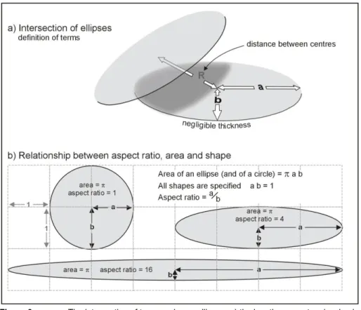
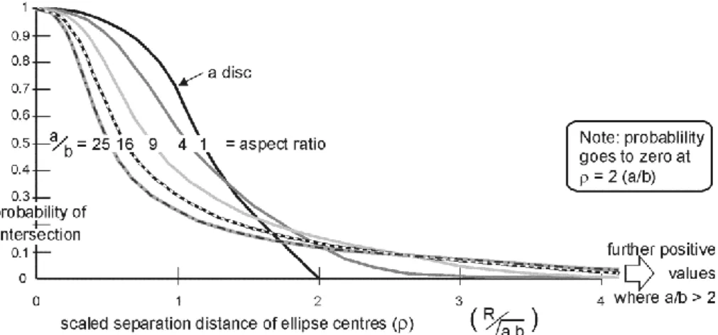
In an effort to understand how fracture shape affected network performance, the study by Black et al., 2007, began by considering the behaviour of intersecting ellipses. Ellipses were investigated because they can be continuously altered from an (equi-dimensional) circular disc into an extremely eccentric ellipse that is very similar to a (one-dimensional) channel (Figure 9).
Figure 9 The intersection of two equal area ellipses a) the length parameters involved
in the assessment of the probability of intersection [the angle parameters are omitted]. b) the use of aspect ratio to ‘evolve’ an equi-dimensional disc into a one-dimensional channel.
The simplest starting point was to examine the probability of intersection of two ellipses of equal area placed at two random locations at two random orientations. The results (Figure 10) are largely as expected in that as the separation distance increases the probability of intersection decreases and goes to zero once separation distance exceeds twice the major axis. For a disc this is twice the radius. The interesting aspect of Figure 10 is how there continues to be a chance of intersection for ellipses at separation distances where equi-dimensional objects cannot intersect and therefore could ‘span’ larger volumes than discs with the same area.
Figure 10 The probability of intersection of two equal area ellipses as a function of
separation distance.
The next step was to see whether the probability of large separation distance intersection was sufficient to enable a continuous set of intersections across a large region containing multiple randomly placed ellipses. The concept of percolation threshold can be visualised as gradually filling a fixed volume of space with randomly placed ellipses. After each ellipse is placed, the investigator checks whether there is a continuous pathway of intersecting ellipses. The number of ellipses per unit volume when a continuous pathway first appears in half the realisations is termed the percolation threshold.
Clearly, the process of determining the percolation threshold is probabilistic and involves multiple realisations of possible networks. Recent work by Barker (pers. comm.) has shown that what was suspected based on two intersecting ellipses does in fact carry through to the behaviour of networks. The results (Figure 11) show that as discs evolve into channels, the percolation threshold declines from a value of about 0.23 for equi-dimensional discs to a value of 0.05 for 16:1 ellipses. (N.B. where there is an “S” shaped curve of this nature, the 50 percentile is often quoted as the discriminating value.) The results are based on 100 realisations of systems containing 1000 ellipses which are all of the same size and shape. Based on this work, it could be expected that channel based systems could percolate at values of P32 in the order of at least a fifth, and possibly less, of the value for an equi-dimensional system.
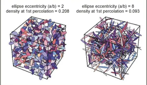
It is relatively straightforward to visualise the difference that this consideration of shape can have on fracture density. Figure 12 shows two ellipse networks, both at the value of density equal to the percolation threshold. Obviously the 8:1 network is not sparse enough to ‘see through’ but the edges show the difference more clearly. A further experiment has been conducted showing that placing the ellipses
orthogonally increases the percolation threshold slightly. Other numerical experiments involving different variations could be readily undertaken.
Figure 11 The variation of percolation with ellipse aspect ratio and area density.
Figure 12 Comparison of two ellipse systems at the values of density equivalent to their
respective percolation thresholds
When viewing Figure 12, it should be borne in mind that not all the fractures depicted participate in throughflow. In fact, early indications are that only about 20 to 40% of the ellipses are active. It should also be borne in mind that the percolation model does not calculate flow, it simply identifies which ellipse is intersected by other ellipses and whether there is a continuous pathway across the network. In order to assess the effect of a channel organisation on flow and head loss within a network, the original study by Black et al., R-07-35, used an orthogonal lattice model named HyperConv. It is described in Black et al., R-06-30. It used two
simple probability functions to generate strings of straight-line connections on a lattice of nodes. The lengths of the strings varied around a central value (controlled by one of the probability functions) whilst the other placed the strings randomly in the lattice. All the connections within a given string had the same conductance and most of the realisations had the same value for all strings.
The lattice model produced the same form of results as Figure 11 (see Figure 13). Of particular note is the result for the shortest channels where the network consists of string lengths of a single connection. It percolates suddenly and at a higher value of density than the longer ones. Since the network is orthogonal, this should equate to an equi-dimensional system.
The lattice model was used to simulate flow into a drift based on measurements at 350m depth in the underground research laboratory at Stripa Mine in the early 1980s. It reproduced most of the effects seen in the old experiments, in particular the formation of a positive skin effect around excavations. Essentially the modelling showed that flow in sparse systems has great difficulty in adhering to the imposition of a boundary condition such as cylindrically convergent flow to a line source (a tunnel or a borehole). This is because the channels are so sparse and active inflow points are few and far between. It was discovered that single channels are likely to be in the order of several metres long and possibly in excess of 10m and must cross many fracture intersections without bifurcating.
Essentially, it’s the density of ‘junctions’ that matters and distinguishes channel flow systems from discrete fracture networks.
Figure 13 Values of channel density around the percolation threshold for varying
Black et al., R-07-35, termed such systems ‘sparse channel networks’. It is the sparseness that yields the characteristic behaviours of ‘skin’ and ‘compartments’ of head and chemistry. Figure 14 illustrates the difference between sparse channel networks and discrete fracture network models such as have been adopted for the SR-Site.
Figure 14 A comparison of a ‘sparse channel network’ simulation using a lattice model
of flow around a drift at Stripa (left image) to a discrete fracture network representation of the TRUE block experiment at Äspö (right image). Both are at similar depths.
3.3.3. The alternative models project undertaken by SKB
SKB considered the use of different model approaches in their study, the Alternative Models Project (Selroos et al., 2002). They published a summary of the project that considered the outcomes from three different types of model of groundwater flow in crystalline bedrock. The three model types were a Stochastic Continuum, a Discrete Fracture Network and a Channel Network. They found that the three approaches yielded similar travel times and fluxes but dissimilar variability. They concluded that the channel network had the lowest spatial variability and that a combination of dfn model at repository scale and stochastic continuum at larger scales was the best compromise.
It should be pointed out however, that the code used, CHAN3D, represented the channel system as a “... network with stochastic conductance values arranged on a rectangular grid ...”
Based on experience with HyperConv, I assume that the effect of the orthogonal grid and the division of flows at every node of CHAN3D was to produce a dense
network of junctions and a result very similar to the other two models. I do not believe that CHAN3D adequately simulated the behaviour of real channel networks.
3.4. Summary of conceptual and numerical modelling
At face value, the SKB conceptual model of bedrock broken up into large blocks by extensive, regional scale deformation zones appears straightforward and intuitive. However, I’m not sure that this division, though reasonably clear-cut geologically is also found within the hydrogeological data. Also, the geological concept carries with it the idea that more extensive features are more important hydrogeologically, more transmissive.
The structural interpretation of the Forsmark site is dependent on the assumption that fractures are equi-dimensional. This is also carried through into the
hydrogeological dfn modelling. Whilst I understand the need to make this assumption when constructing a hydrogeogical dfn model, I believe it leads to predicting too many flow junctions and too many apparently flowing features. The symptom of too many flowing features, despite being very close to the percolation threshold, is seen in Figure 8 (their Fig 11-15 of R-07-48) where the modelling assigns low values of transmissivity to 85% of the ‘flowing’ fractures. This is done so that they have negligible impact on the main matching parameter, total borehole flow rate. The associated problem of having too many predicted flowing features is solved by assigning such low values of transmissivity that they would fail to be recorded by the PFL-f measurement method.
Another symptom of an underlying assumption is also seen in Figure 8 in the form of a small number of higher-than-measured inflows. Since transmissivity is linked to extensiveness by a power law then these inflows must reflect extensive features. I suspect the power law size-transmissivity relationship makes all predictions
sensitive to occasional very extensive features.
In general, I consider the modelling process very complex, particularly the parameterisation, and it is difficult to link outcomes to inputs. I am still uncertain about what value of ‘large-scale hydraulic conductivity’ to associate with the hostrock volume, FFM01.
Overall, I suspect that the modelling is reasonably accurate for the more fractured regions of the target area. On the basis of the comparisons of modelled versus measured, I consider the agreement for FFM01 below 400m depth to be poor. In particular, I suspect the model is a poor predictor of hostrock behaviour at the 5-10m scale.
4. Checking measurements
4.1. Introduction
It is important in groundwater modelling to have some independent measurements that can be predicted by the model and yet aren’t part of the calibration process. The more complex the modelling, the more important these ‘checking’ measurements are. I list the usual candidates in Figure 3:
1. Water balance
2. Head distribution within the modelled region
SKB recognise the need for such measurements in the development of the “bedrock hydrogeological model” and provide the following list on page 230 of TR-0805 “As a means of approaching the issue of confirmatory testing, a strategy was developed after the initial site investigation (ISI) stage /Follin et al. 2007a/, see Figure 8‑2. In practice, four kinds of data were treated during the complete site investigation (CSI) stage:
A. Hydraulic properties deduced from single-hole hydraulic tests (double-packer injection tests, PSS, difference flow logging pumping tests, PFL-f, and open-hole pumping tests combined with impeller flow logging, HTHB) /Follin et al. 2007b/.
B. Groundwater level responses (point-water head drawdowns) in the bedrock in the depth interval 0 to c. 700 m observed during large-scale interference (cross-hole) tests /Follin et al. 2007c, 2008a/.
C. Present-day mean groundwater levels (point-water heads) observed in the Quaternary deposits and the uppermost (c. 150 m) part of the bedrock /Follin et al. 2007c, 2008a/.
D. Hydrochemical data (fracture water and matrix porewater) gathered from the bedrock investigations (primarily the core-drilled boreholes) /Follin et al. 2007c, 2008a/.”
The SKB measurements could be summarised as: 1. the distribution of transmissivity
2. drawdown responses to large scale pumping tests 3. the water table
4. chemistry of the groundwater
A water balance is not on the list because it would be irrelevant to the development of a bedrock model since it would be dominated by the transmissive near-surface rocks and soil zone. However, the items at 2 and 3 are also irrelevant to bedrock modelling. Item 1 is partly used to calibrate the model and has been discussed in Section 3.2 above. The main checking parameter is undoubtedly the distribution of groundwater chemistry.
The notable omission from SKB’s checking measurements is head: namely the natural variation of head that is likely to be found in situ. Most programmes of this type measure it and it is usually extremely enlightening if difficult to explain. It often reflects processes that haven’t been included in any modelling.
SKB do report some head measurements from long term monitoring but they are from long sections of the cored boreholes. The reports, such as Nyberg and Wass, P-09-42, record time series data from all monitored boreholes in the target area without interpretation. The monitoring has two major drawbacks. The monitored sections are generally very long with many over 100m long. Where they are shorter it is usually because of the presence of a deformation zone. There is likely to be mixing occurring continuously within the longer intervals. The second drawback is that the monitoring intervals are measured by tubes to the surface and near-surface based transducers. The tube to depth contains water of unknown density so environmental water heads are not possible to deduce with any certainty. All is not lost though, since the PSS method recorded heads with downhole transducers during the reasonably comprehensive straddle-packer testing in the cored boreholes. SKB make no use of the measurements but record some rudimentary heads in their Sicada database.
I have extracted head data from their PSS reports and the Sicada database.
4.2. Heads from the straddle-packer testing
4.2.1. Extracting values of head from the PSS testing
The PSS testing took the form of straddle packer injection tests with an injection duration of 20 minutes at an imposed head of about 20m of water. The procedure is illustrated in Figure 15 showing a 20 minute period after packer inflation for the test zone to equilibrate before the start of injection. After injection stopped a further 20 minutes was allowed for equilibration towards whatever was the environmental head of the test zone at equilibrium. The packers were then deflated regardless of
whether the zone had regained equilibrium. The head was recorded at P1, P2 and P3 and entered into SKB’s Sicada database. Naturally, tests varied and ideally P1 and P3 would be equal. For an initial assessment, I picked the value for P1 out of the tables at the back of the PSS field reports.
Figure 15 A typical PSS test annotated to show pressure events within the test zone
4.2.2. Converting pressure to environmental head
Comparing two or more values of head indicate the direction of groundwater movement. In general terms, comparing ‘freshwater’ heads at three points of equal elevation indicates the direction of horizontal flow and comparing ‘environmental water heads’ measured at different points in a vertical borehole yields the direction of vertical flow. ‘Environmental water head’ is ‘freshwater head’ compensated for density variations in the water column above the measurement point.
To convert the measured pressures to environmental head I had to: 1. Remove 100KPa to account for atmospheric pressure
2. Identify the exact elevation of the transducer measuring the test zone (surprisingly uncertain but based on the corrected borehole trajectories in P-07-28 and unravelling the inconsistencies in the PSS reports)
4. Correct for the effect of temperature and pressure on density
Ultimately, I derived a set of freshwater and environmental water heads for all the boreholes tested by the PSS system. Values of freshwater head are of little interest. The results are included as Appendix 4 to this report within an Excel spreadsheet.
4.2.3. Environmental heads in the KFM boreholes
The environmental heads derived from the PSS tests are very interesting. Naturally, the short-term nature of the testing is a significant effect and low transmissivity intervals don’t have time to gain or regain equilibrium. A typical results set is shown in Figure 16. One of the characteristics of the results overall is that the 100m intervals average out minor head variations both because they average out variations in situ and because being longer they have a higher transmissivity than the shorter sections and therefore approach equilibrium more quickly. Essentially they regain equilibrium in the 20 minutes available. The problem of not regaining equilibrium becomes more prevalent amongst the results as interval length declines and the ‘spikey’ nature of the 20m and 5m results is the outcome. Overall, KFM3A & B exhibit a small upward head gradient.
Figure 16 A typical set of PSS head results
Several points should be borne in mind:
the density correction at 1000m depth is about 6m of water head meaning that up to 6m of head has already been subtracted from the results in Figure 16.
The transducer is located at the top of each interval so each datapoint applies to the appropriate length of borehole beneath it. This is most marked in the 100m long intervals
The dataset has many intriguing results. For instance two thirds of the profiles feature a divergence between the 100m interval results and the shorter interval tests. One such is KFM09A. The shorter interval tests appear to indicate a small upward gradient whereas the 100m results indicate the opposite. There may well be an obvious practical explanation such as a long period of prior pumping since the 100m tests were usually performed first.
I have also added a rough average of a sample of data from the monitoring report (P-09-42). Although it represents long sections of borehole and the values are most likely ‘freshwater heads’, they represent downward flow to depth. Topographically driven flows would normally result in raised heads at depth in boreholes in the discharge area, i.e. near to the coast.
In an effort to get some general relationships from the data, I decided to form the results sets into groups: downward flowing , neutral and upward flowing. They are presented below as Figures 18, 19 and 20.
Figure 17 PSS head results from KFM09A plus some roughly averaged heads from the
Figure 18 The ‘downward flowing’ PSS head results.
Figure 20 The ‘upward flowing’ PSS head results
There are many inconsistencies in these results which may well be resolved by a thorough examination of each test and the addition of knowledge derived from the long term monitoring.
Whatever the outcome, it is unlikely that the head profiles at depth are the result of the present-day topographically driven flow that dominates near the surface.
4.2.4. Causes of head variations at depth
The most likely cause of head variations at depth, particularly negative heads, is relic pressures arising from the glacial history. SKB summarise the glacial history in terms of a graph of ice sheet depth, permafrost thickness and sea level change (Figure 20). It shows a glacial maximum only 8,000 years ago and an ice sheet thickness of more than one kilometre persisting for more than 10,000 years. SKB also estimate a groundwater head of 80% of ice sheet thickness applied to the top of the groundwater system. After this long period of applying a considerable weight, the ice melted quite sharply and the bedrock will have dilated following the long period of consolidation.
Figure 21 A schematic summary of the glacial history at Forsmark
The rate of dilation or consolidation is related to the bulk hydraulic conductivity of the bedrock. I have therefore calculated using consolidation theory the amount of head that might remain at depth in the bedrock based on some rough estimates (see Figure 21). It appears that a value of bulk hydraulic conductivity of about 1x 10-11 m/s represents the threshold when one might expect to observe relic heads from the last ice age.
Figure 22 An assessment of the possible influence of the last ice age on head
conditions in the bedrock at Forsmark.
4.3. Heads in the modelling
Heads are seldom if ever mentioned in the modelling reports except in regard to the near surface layers and the response to pumping tests. Indeed in the report
concerning the modelling of the glacial period (Vidstrand et al., R-09-21), the authors identify their confirmatory data as:
“transient, large-scale cross-hole (interference) test responses,
steady-state, natural (undisturbed) groundwater levels in the uppermost 150 m, and
hydrochemical observations in deep boreholes.”
It is unclear from the Vidstrand et al., R-09-21 report what is the head distribution in the bedrock at the end of the glacial period, i.e. the present day. There is also the remark in TR-10-48 that the ConnectFlowTM code has the advantage that it passes the boundary conditions from the district model to the repository scale model “so that it is not necessary to explicitly transfer boundary conditions between different models”.
In the absence of information to the contrary, I assume that the only information on the vertical boundaries surrounding the repository model are essentially hydrostatic taking account of the density variation due to the increase in salinity with depth. Whilst this might apply to the deformation zones, I doubt it applies to the background rock of the repository volume. Indeed the difference between pore water and fissure water chemistry would seem to support that conclusion.
5. The hydrogeology of EDZs
I note the inclusion of high values of hydraulic conductivity in the modelling in relation to the Excavation Damaged Zone (EDZ). I have checked the report by Bäckblom, TR-08-08 summarising previous experiments and take issue with the conclusions drawn there that the experiments at Stripa reported by Börgesson et al, 1992 produced results of any reliability. The report is the first to mention a
hydraulic conductivity value of 1x10⁻⁸ m/s for the EDZ which seems to have become folklore. This value resulted from the misapplication of a porous medium model in fractured rock based on insupportable assumptions.
To the best of my knowledge, beyond a few centimetres of blast damage, the permeability of an EDZ has never been measured hydraulically in a non-spalling environment.
6. Discussion and conclusions
Investigating the subsurface is always uncertain. The hydrogeology of sparsely fractured crystalline rock at depth is a case in point. Forming conclusions is largely a question of believing or not believing the arguments put forward within a reasoned interpretation. Conclusions are most easily arrived at if there are multiple lines of evidence.
In that context, I believe the SR-Site hydrogeological approach has gathered insufficient ‘checking’ evidence relevant to the hostrock, FFM01.
Most modelling projects in the world of hydrogeology use historical measurements to check the validity of their model’s behaviour. In this case, where head and water chemistry are the evidence of history, head has been virtually omitted from
measurement or reporting.
Forming conclusions is made more than averagely difficult when stochastic modelling is being used as in this project. The dfn method is particularly intricate
and includes many assumptions that are questionable, such as the size-transmissivity relationship and equi-dimensional (hydraulically active) fractures.
I believe the dfn models in SR-Site are at their percolation limit when applied to the host rock and that the host rock is actually below that limit. I have proposed a conceptual model above which would address that problem. However, this is not to say that the host rock does not have desirable hydrogeological properties, simply that the current model does not appear to be a good predictor of its behaviour. I believe that the host rock has lower bulk flow rates, as high or higher flow
velocities, lower ‘fracture wetted surface’ and sparser flowing features than the SKB dfn model.
Linked to uncertainty in the characteristics of the potential host rock is the question of the lower measurement limit of the field testing. It is unfortunate that the measurement limit of both techniques seems to be so high that almost 50% of the actively flowing features of the host rock occur just below the limit (according to SKB’s own model)
I believe the lower limit is too high for the purposes of gaining confirmatory evidence about the host rock.
In general, I think the site characterisation doesn’t place enough emphasis on measuring and modelling the host rock hydrogeologically.
7. Non SR-Site references
Black, J.H., Robinson, P.C. and Barker, J.A. 2006. A preliminary investigation of the concept of hyper-convergence. Report of SKB. Research Report, R-06-30, 66pp.
Black, J.H., Barker, J.A. and Woodman, N. 2007. An investigation of ‘sparse channel networks’ – characteristic behaviors and their causes Report of SKB. Research Report, R-07-35, 123pp.
Gale, J.E. 1981. Fracture and hydrology data from field studies at Stripa, Sweden. Report of Lawrence Berkeley Laboratory, Univ. Of California, No LBL-1310, pp. 270.
Robinson, P.C. 1984Connectivity of fracture systems - A percolation theory approach, J. Phys. A, Math. Gen., 16, 605-614.
Selroos, J.-O., Walker, D.D., Strom, A., Gylling, B., and Follin, S., 2002.
Comparison of alternative modelling approaches for groundwater flow in fractured rock.Journal of Hydrology, 257, pp 174-188
Appendix 1
Coverage of SKB reports
Table 1 Top level reports
Reviewed report Reviewed sections Comments
TR-11-01 Main report of the SR-Site project
as required by contract reasonably clear TR-10-48 Geosphere
Process report
3.1, 5.2 and 6.1 uncertain as to purpose TR-10-52 Data Report 6.3,6.6 and 6.7 one of the main sources
TR-10-49 3.2 much speculation
Table 2 Main useful reports
Reviewed report Reviewed sections Comments
TR-08-05 Site description of Forsmark etc
2.3,2.4,3-5, 811.6& 11.7 useful R-09-21Gw flow modelling of
periods with periglacial
most sections R-09-22 SR Site gw flow
modelling methodology etc
most sections R-07-48 Hydrogeological characterisation etc most sections R-07-49 Hydrogeological conceptual model development etc
sections on rock domains
R-08-95 Site descriptive modelling etc
sections on fracture domains
Table 3 less useful reports
Reviewed report Reviewed sections Comments
R-01-51 Methodology study of Posiva flow meter R-08-23 Hydrogeological conceptual model development R-08-10 Presentation of meteorological , hydrological etc