2004:02 Two Dimensional Near-field Calculations of Radionuclide Releases from the Vaults of the SFR 1 Repository

SKI Report 2004:02

Research

Two Dimensional Near-field Calculations

of Radionuclide Releases from the Vaults

of the SFR 1 Repository

António Pereira

Benny Sundström

December 2003

SKI perspective

Background

As part of the license for SFR 1 a renewed safety assessment should be carried out at least every ten years for the continued operation of the SFR 1 repository. Around mid 2001 SKB finalised their renewed safety assessment (project SAFE) which evaluates the performance of the SFR 1 repository system.

As part of SKI’s own capability to perform radionuclide transport calculations a need to develop a two-dimensional (2D) near-field model of the SFR 1 repository was identified.

Purpose of the project

The purpose of this project is to investigate the possibility to develop a useful two-dimensional radionuclide transport near-field model of the vaults in the SFR 1 repository. The results from the 2D model are compared with the calculated radio-nuclide release from the vaults of SFR 1 done by SKB in their project SAFE. Results

For most of the studied calculation base cases there is a relatively good agreement with SKB results. Calculation cases where the agreement with SKB results is not so good are mostly for the carbon radionuclide. There may be several explanations for this disagreement. However, to solve this a thorough investigation is needed. Inspite of the obtained disagreement for the carbon-calculation cases, the 2D model concept

developed in this project is, on the whole, applicable to the vaults of the SFR 1 repository.

Project information

Responsible at SKI has been Benny Sundström. SKI ref.: 14.9-010636/01108

SKI Report 2004:02

Research

Two Dimensional Near-field Calculations

of Radionuclide Releases from the Vaults

of the SFR 1 Repository

António Pereira¹

Benny Sundström²

¹Department of Physics

AlbaNova University Center

Stockholm Center of Physics, Astronomy and Biotechnology

SE-106 91 Stockholm, Sweden

²Swedish Nuclear Power Inspectorate

SE-106 58 Stockholm, Sweden

December 2003

This report concerns a study which has been conducted for the Swedish Nuclear Power Inspectorate (SKI). The conclusions

Contents

2.2 The BMA vault ... 8

2.3 The BLA vault ... 9

2.4 Waste inventory ... 9

2.5. Barrier properties and data... 10

2.5.1 Material and nuclide data used in the calculations ... 10

2.6 Hydrology and host rock data... 11

3. VAULT MODELLING... 15

3.1 The conceptual model... 15

3.2 Assumptions and model simplifications ... 16

4. BASE CASE... 19

4.1 Introduction... 19

4.2 The 2BTF vault... 19

4.2.1 Description of the barriers... 19

4.2.2 Results ... 21

4.3 The 1BTF vault... 25

4.3.1 Description of the barriers... 25

4.3.2 Results ... 27

4.4 The BMA vault ... 31

4.4.1 Description of the barriers... 31

4.4.2 Results ... 32

4.5 The BLA vault ... 37

4.5.1 Description of the barriers... 37

4.5.2 Results ... 38 5. COMPLEXING AGENTS... 43 5.1 2BTF ... 43 5.2 1BTF ... 44 5.3 BMA ... 45 5.4 BLA ... 46 6. VARIABILITY STUDIES... 47

6.1 The impact of fractures on the radionuclide release ... 47

6.2 The impact of the Darcy flow on the radionuclide release ... 47

6.3 The impact of a large fracture in the concrete barriers ... 49

6.3.1 2BTF results ... 49

6.3.2 1BTF results ... 54

6.3.3 BMA results ... 56

7. SUMMARY AND CONCLUSIONS... 59

REFERENCES... 61

APPENDIX I... 63

Abstract

Radionuclide releases from the near-field for the vaults of the SFR 1 repository are examined in this report. To model those releases we have developed four models, one for each of the vaults; 2BTF, 1BTF, BMA and BLA. The respective codes are based on the finite element method and are called FEMBTF2, FEMBTF1, FEMBMA and

FEMBLA, respectively. These codes are two-dimensional representations of the cross sections of the vaults. The different barriers of the vaults have been modelled

individually using the physical dimensions of the cross sections. The same conceptual model has been used to estimate the releases from the near-field. This conceptual model is implemented by four different FEM codes that solve the two-dimensional transport equation, e.g. the advective-diffusive-reactive equation that also includes radioactive decay. An interesting property of the codes is that they allow the use of time-dependent properties to represent for instance the evolution of water flow, porosities, distribution coefficients etc. This capability of the code has been used only in some cases because the FEM codes put heavy requirements on the computer’s CPU.

The nuclides studied here were chosen from a set representing the highest release rates from the near-field obtained by SKB during their project SAFE. Some of the results reported here are somewhat lower than SKBs, other higher. Uncertainties in the conceptual models and differences in the input data are the reasons for the numerical differences. For most cases, the differences between our results and those of SKB should be considered relatively small within present context of near-field calculations.

Sammanfattning

En analys görs av utsläpp av vissa radionuklider från närområdet för tunnlarna i

SFR 1-förvaret i närheten av Forsmark. För att modellera utsläppet har vi i detta arbete utvecklat fyra modeller för var och en av tunnlarna, 2BTF, 1BTF, BMA och BLA. Modellerna som baseras på finita element metoden heter FEMBTF2, FEMBTF1, FEMBMA och FEMBLA. De utgör tvådimensionella representationer av tunnlarnas tvärsnitt. Tunnlarnas olika barriärer har modellerats individuellt utifrån tvärsnittens fysiska dimensioner. Samma konceptuella modell har använts för att uppskatta utsläpp från närområden. Den konceptuella modellen har översatts till fyra olika numeriska program som löser den tvåldimensionella transport-ekvationen, dvs. den advektiva-dispersiva-reaktiva ekvationen som också modellerar radioaktivt sönderfall. En

intressant egenskap hos programmen är dess förmåga att modellera rumsvariationer och tidberoende egenskaper, t.ex. tidsutveckling av vattenflödet, porositet, etc. Denna förmåga har dock använts sparsamt pga. att finita element program är väldigt CPU krävande.

De nuklider som har studerats är några av de som står för de högsta utsläppen som SKB fick under projektet SAFE. Några av de resultat som rapporteras här är något lägre än SKBs, andra är högre. Osäkerheter i konceptuella modeller och skillnaden i ingångsdata förklarar dessa numeriska diskrepanser. I detta sammanhang är skillnaderna mellan våra resultat och SKB:s att betrakta i de flesta fall som relativt små.

1. Introduction

The SFR 1 is a repository for low and intermediate level waste that is generated by the Swedish nuclear power program and by the research centre at Studsvik, hospitals, universities, etc . The repository is situated at Forsmark in Uppland and consists of one silo and four rock vaults. The vaults have different designs, one is aimed at disposal of medium level waste (BMA), two are for waste sealed in concrete tanks (1BTF and 2BTF) and one for low level waste (BLA).

The repository is constructed below the Baltic sea and during a first period of the repository’s history the sea is the main recipient for the radionuclides that may escape from it. This period is called the saltwater period by SKB in earlier safety studies. Due to land uplift a new biosphere environment will develop during the next following period (the inland period) and therefore a complete set of assessment calculations would require the time evolution of the biosphere. This work is restricted to the performance of the near-field barriers using some radionuclides within the context of a specific set of cases. We report the development of four FEM codes to model the 1BTF, 2BTF, BMA and BLA vaults of SFR 1 in two dimensions and we use them to make estimations of radionuclide releases from those vaults. The calculations cover the saltwater period (following the repository closure) and the inland period without distinction of those periods. The calculations are deterministic and done for a base case scenario and some variations of it.

In the Section Two we describe briefly the SFR 1 vaults and we table the list of

radionuclides in the waste already disposed of (or to be disposed of in the future) in the vaults, together with their respective inventory at year 2030. We also describe shortly the system of barriers and the geometry of the vaults together with data on the material used in the physical barriers. In Section Three we describe the conceptual models used in the calculations and the general assumptions embedded in these models. Section Four presents for each of the vaults, the results of the calculations of the base case. In Section Five the influence of complexing agents on the performance of the system is studied; the same set of radionuclides used in the base case is also used in this case. Section Six on variability studies presents some calculations for a conservative scenario in which a fracture is developed in such a way that it connects the base of the vaults to the top filling. The summary and conclusions are presented in Section Seven, followed by the references and appendixes.

2. The SFR 1 system of vaults

A general layout of the SFR1 repository is shown in figure 2.1. The system consists of a silo and of four vaults. The position of the silo and of the different vaults is labelled for clarity reasons. The two BTF vaults are denominated 1BTF and 2BTF in the text.

Figure 2.1 A sketch of the SFR 1 repository. Of the two BTF vaults, the 1BTF vault

is the left one in the picture (© SKB).

2.1 The BTF vaults

The BTF vaults are aimed at low-level waste. They consist of two vaults (1BTF and 2BTF). In the 1BTF vault, which is for concrete tanks, the material to be disposed off is graphite, ashes, ion exchange resines and scrap. All material is conditionated except the material in the concrete tanks. Approximately 1% of the total activity of SFR 1 will be disposed of in this vault. The 2BTF vault is aimed at deposition of ion exchange resins and the total activity content is also approximately 1% of that of SFR 1.

Figure 2.2 shows a vertical cross section of the 2BTF vault perpendicular to the

longitudinal axis of the vault. The vault is 160 m long, 14.7 m wide and 9.5 m high. The vault walls are covered with a 5-10 cm thick layer of shotcrete. The floor of the vault is of concrete, 0.3 m thick. The tanks in the vault are piled two tanks on the top of each other and four side by side and the space between them is filled with porous concrete. At the top of the tanks a lid of concrete functions as a protection against radiation. The backfill in the top may consist of crushed rock and sand. The 1BTF vault has the same geometry as 2BTF but the waste content is not so homogeneously distributed as in former vault which will be reflected in the way that 1BTF is modelled in this work.

SILO

1BTF

BMA

BLA

2.2 The BMA vault

The BMA vault (figure 2.3) is aimed at disposal of ion-exchange resins, scrap and trash conditionated in cement (76%) or bitumen (24%). About 55% of the waste volume is ion-exchange resins, scrap and trash covering the remaining 45%. These wastes are conditioned in cement or bitumen. The activity content is relatively high although lower than in the Silo. Approximately 6% of the total activity content of SFR 1 is found in BMA.

The BMA vault is 160 m long, 19.6 m wide and 16.5 m high (figure 2.3). The vault is divided in 13 large wall sections of concrete. For details the reader should consult SKB´s compilation of data (SKB, November 2001).

Radiation protection lid (concrete) 14.7 9.5 Rock Vault backfill Permeable concrete Waste package Concrete bottom plate Waste Permeable concrete

2.3 The BLA vault

The BLA vault (figure 2.4) is for low-level waste and it is constructed to take care of metallic materials, cellulose and other organic materials. A total of approximately 0.1% of SFR 1 activity content will be found here.

2.4 Waste inventory

The nuclides studied are C-14 (organic), C-14 (inorganic), I-129, Ni-59 and Cs-135 representing high releases from the near-field according to the SKB calculations done within their project SAFE. The nuclides disposed of in the four SFR 1 vaults, their half-life and their activity content are shown in Table 2.1 (Lindgren et. al, October 2001; Riggare et. al., June 2001).

Table 2.1 Radionuclide content of the SFR 1 rock vaults (year 2030).

Element Half-life (year) 1BTF (Gbq) 2BTF (Gbq) BMA (Gbq) BLA (Gbq) 14_Corg. _5.7×103 _1.8×102 _3.0×101 _1.7×102 _3.3×10-2 14_Cinorg. _5.7×103 _2.3×103 _2.7×102 _1.9×103 _3.9×101 59_{Ni 7.5×10}4 _1.8×102 _3.0×102 _2.1×103 _3.9×101 129_{I 1.6×10}7 _9.1×10-3 _1.6×10-2 _1.0×10-1 _2.5×10-3 135_{Cs 3.0×10}6 _1.5×10-1 _2.7×10-1 _1.7×100 _4.1×10-2

Figure 2-4 A sketch of the cross section of

the BLA vault.

Figure 2-3 A sketch of the cross section of

the BMA vault.

16.5 m

19.6 m

12.5 m

2.5. Barrier properties and data

2.5.1 Material and nuclide data used in the calculations

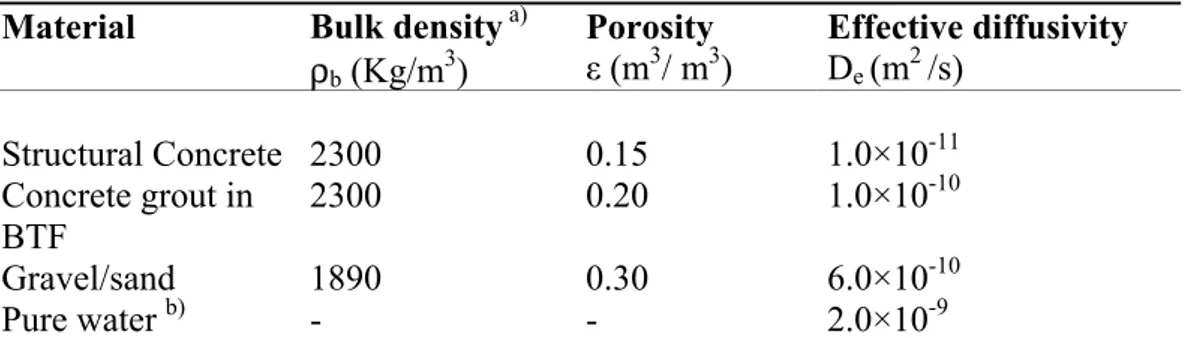
The data on the physical and chemical properties of the different materials used in the construction of the repository, which are of relevance for our calculations, are given in this section. They are needed as input data to the radionuclide release codes developed for use in our calculations. Table 2.2 gives the densities, porosites and diffusivities for the different materials used in the construction of the vaults (SKB, November 2001). The solid density is computed from the bulk density. Table 2.3 gives the distribution coefficients (sorption coefficients) of the radionuclides in concrete and cement (SKB, November 2001).

Table 2.2 Densities, porosities and diffusivities for the materials used in the SFR 1

vaults.

Material Bulk density a)

ρb (Kg/m3) Porosity ε (m3/ m3) Effective diffusivity De (m2 /s) Structural Concrete 2300 0.15 1.0×10-11 Concrete grout in BTF 2300 0.20 1.0×10-10 Gravel/sand 1890 0.30 6.0×10-10 Pure water b) - - 2.0×10-9

a) _{The bulk density is given by ρ}

b = ρs (1-ε) where ρs is the solid density.

b) _{The diffusivity data for water (all ions) is included here for the sake of completeness.}

Table 2.3 Sorption coefficients, Kd, (m3/kg). Ox. State1) Element Concrete

and cement

M(II) Ni 0.04

C(inorg.) 0.2

C(org.) 0

I 0.003

Table 2.4 Sorption coefficients on rock fill (sand/gravel).

Ox. State 1) Element Kd (m3/kg)

M(I) Cs 0.01

M(II) Ni 0.01

C(inorg.) 0.0005

C(org.) 0

M(-I) I 0

1)_{oxidation state for major ionic species at reducing Eh and pH 7-14.}

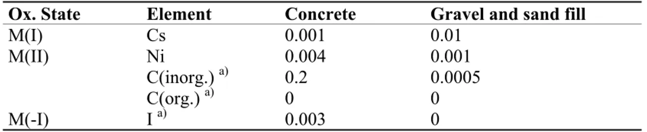
Table 2.5 Sorption coefficients for calculation cases with impact of complexing agents.

Ox. State Element Concrete Gravel and sand fill

M(I) Cs 0.001 0.01

M(II) Ni 0.004 0.001

C(inorg.) a) 0.2 0.0005

C(org.) a) _{0 0}

M(-I) I a) 0.003 0

a) _{not affected by complexing agents.}

Table 2.4 gives sorption coefficients on rock fill (SKB, November 2001). The impact of complexing agents on the sorption of nuclides on concrete and gravel/sand is given in Table 2.5 (SKB, November 2001).

2.6 Hydrology and host rock data

The hydrogeological data needed for our near-field calculations is taken from the modelling of future hydrogeological conditions of SFR 1 (Holmén and Stigsson, 2001a).

The total water flow and the average specific flow vary with time according to the

values given in Tables 2.6 and 2.7 respectively1_{. These tables are for the different parts}

of the vaults of SFR 1.

Table 2.6 Total flow in the different parts of the repository.

Total water flow rate on the top filling

(m3/year)

Time BTF1 BTF2 BLA BMA

0 6.6 5.9 10.1 5.9 1000 17.4 14.2 15.1 20.6 2000 24.3 25.1 32.5 33.8 3000 27.4 26.8 36.5 35.4 4000 28.1 27.2 37.1 35.5 5000 28.1 27.2 37.1 35.5

An illustration of the time variation of the total flow in the top filling of the vaults is given in figure 2.5 using the data given in Table 2.6. These data are fitted (figure 2.6)

using the logistic equation (Equation 2, section 3.1) with 3 variable parameters, k1, k2

and k3.

Figure 2.5 Total flow through the top filling of the four SFR 1 vaults. The time scale

starts when the repository is closed.

That variation with time of the total water flow is included in the models. In fact it is possible to include time dependency of all parameters in our models although this has not been done either than in the case of the total water flow to avoid very time

consuming calculations.

BTF1 BTF2 BLA BMA

Total flow on the top filling of the SFR-1 vaults

Time (years)

Total flow (m3/year)

0 5 10 15 20 25 30 35 40 0 1000 2000 3000 4000 5000

Figure 2.6 The logistic model fitted to the total flow through the top filling of the four

SFR 1 vaults. The time scale starts when the repository is closed. Time (years)

Total flow (m3/year)

0 6 12 18 24 30 0 1000 2000 3000 4000 5000 BTF2 k1=27,56158422 k2=4,41507459 k3=0,0016919697 Time (years)

Total flow (m3/year)

0 6 12 18 24 30 -500 500 1500 2500 3500 4500 5500 BTF1 k1=28,11163783 k2=3,117642829 k3=0,0015675788 Time (years) T otal fl ow ( m 3/y ear ) 0 5 10 15 20 25 30 35 40 45 -500 500 1500 2500 3500 4500 5500 BLA k1=38,19457395 k2=4,237377668 k3=0,0013829681 Time (m3/year)

Total flow (m3/year)

-5 0 5 10 15 20 25 30 35 40 -500 500 1500 2500 3500 4500 5500 BMA k1=35,797549 k2= 5,597589204 k3=0,0020848598

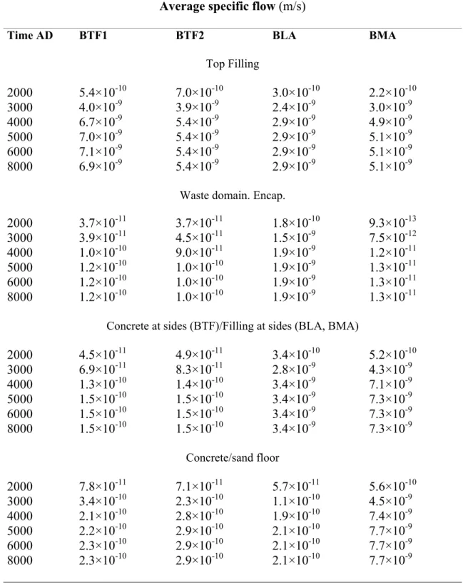
Table 2.7. Average specific flow at different times, in the different parts of the

repository vaults.

Average specific flow (m/s)

Time AD BTF1 BTF2 BLA BMA

Top Filling 2000 5.4×10-10 7.0×10-10 3.0×10-10 2.2×10-10 3000 4.0×10-9 3.9×10-9 2.4×10-9 3.0×10-9 4000 6.7×10-9 5.4×10-9 2.9×10-9 4.9×10-9 5000 7.0×10-9 5.4×10-9 2.9×10-9 5.1×10-9 6000 7.1×10-9 5.4×10-9 2.9×10-9 5.1×10-9 8000 6.9×10-9 5.4×10-9 2.9×10-9 5.1×10-9

Waste domain. Encap.

2000 3.7×10-11 3.7×10-11 1.8×10-10 9.3×10-13 3000 3.9×10-11 4.5×10-11 1.5×10-9 7.5×10-12 4000 1.0×10-10 9.0×10-11 1.9×10-9 1.2×10-11 5000 1.2×10-10 1.0×10-10 1.9×10-9 1.3×10-11 6000 1.2×10-10 _1.0×10-10 _1.9×10-9 _1.3×10-11 8000 1.2×10-10 1.0×10-10 1.9×10-9 1.3×10-11

Concrete at sides (BTF)/Filling at sides (BLA, BMA)

2000 4.5×10-11 4.9×10-11 3.4×10-10 5.2×10-10 3000 6.9×10-11 8.3×10-11 2.8×10-9 4.3×10-9 4000 1.3×10-10 1.4×10-10 3.4×10-9 7.1×10-9 5000 1.5×10-10 1.5×10-10 3.4×10-9 7.3×10-9 6000 1.5×10-10 1.5×10-10 3.4×10-9 7.3×10-9 8000 1.5×10-10 1.5×10-10 3.4×10-9 7.3×10-9 Concrete/sand floor 2000 7.8×10-11 7.1×10-11 5.7×10-11 5.6×10-10 3000 3.4×10-10 _2.3×10-10 _1.1×10-10 _4.5×10-9 4000 2.1×10-10 2.8×10-10 1.9×10-10 7.4×10-9 5000 2.2×10-10 2.9×10-10 2.1×10-10 7.7×10-9 6000 2.3×10-10 2.9×10-10 2.1×10-10 7.7×10-9 8000 2.3×10-10 2.9×10-10 2.1×10-10 7.7×10-9

3. Vault modelling

3.1 The conceptual model

The vaults and the release of radionuclides from the near field are modelled as 2D finite element sections perpendicular to the longitudinal axis of the vaults. The radionuclide release from the vaults is assumed to be controlled by advection and diffusion. The rates of diffusion through the different parts of a vault are expressed by the diffusivities of the respective materials and may differ from each other (for instance porous concrete and gravel/sand have different effective diffusivities for the same nuclide). The conduc-tivities of the barriers are different and the water flow through those barriers varies in time. The vaults are modelled by a system of partial differential equations, together with the logistic equation, which expresses the time variation of the water flow through the top filling (figure 2.6). The dimensions of the 2D cross sections (length and width) of the barriers used in the model are the same as the corresponding physical barriers (SKB, November 2001) which means that no equivalent barriers are considered. This approach makes the modelling as transparent as possible. There is one exception for the 1BTF vault where one equivalent barrier was introduced to simulate the retardation effect of the concrete in drums containing waste.

The model takes into account that fractures will develop in the concrete of the tanks and walls. This is done in two different ways; first by using values for the hydraulic conduc-tivity of each barrier that are equivalent to the existence of a certain number of fractures per meter and second by introducing into the model a physical fracture in the barrier connecting the waste with the backfill (see for instance figure 4.1 in section 4.2). The model simulates the two-dimensional advective-diffusive-reactive processes and the radioactive decay (Equation 3.1) together with the time-dependent variation of the total water flow

/ t R c( ) . ( D c c u ) R c (i 1... )n (3.1) i i i i i i λi i i

∂ ∂ + ∇ − ∇ + = − =

in top filling (Equation 3.2) by:

with: ) 3 . 3 ( ) 1 ( 1 i i i i i Kd R ε ε ρ − + = and where:

i - is the label of a zone in the 2D integration domain, Ω. n - number of zones in the domain Ω.

Ci (x,y,t) - is the radionuclide concentration in pore water in zone i, (Bq/m3).

Ri - is the retardation coefficient in zone i, (-).

( ) ₁ /(1 ₂ exp( ₃ )) ˆ (3.2)

u t k _i k _i k t_i u

ρi - is the density in zone i, (kg/ m3)

εi - is the porosity in zone i, (-).

Kd,i - is the distribution coefficient in zone i, (m3/kg).

Di - is the effective diffusivity in zone i, (m2/year).

t - is the time (years)

λ - is the radioactive decay constant, (year)-1

ui (x,y,t) - is the darcy velocity in zone i, (m/year)

k1 i - is the first constant of the logistic equation, (-)

k2 i - is the second constant of the logistic equation, (-)

k3 i - is the third constant of the logistic equation, (-)

The advective and diffusive processes included in the model are illustrated by figure 3.1. The initial and boundary conditions are described in the sections dealing with the respective models of the BTF, BMA and BLA vaults. Multiplying the activity

concen-tration (Bq/m3) by the water flow (m3/yr) in the different zones, one obtains the

respec-tive release rates (Bq/yr). These are summed to obtain the total release rate from the vault. The conceptual model described here is implemented into the two-dimensional commercial 2D program FlexPDE (version 2). An example of the script code used in FlexPDE for the vault 2BTF is described in appendix I.

3.2 Assumptions and model simplifications

The assumptions are related to the fact that the finite element model expressed by the system of coupled partial differential equations with time varying groundwater

velocities (Darcy velocities) requires computer CPU times of the order of 36 hours for each run. The straightforward approach to reduce the CPU time (in some cases by orders of magnitude!) is to assume that the average specific flow was constant with time and to make eventually two variation studies for each nuclide where the flow is assumed to have its minimum value in one case and its maximum value in another case and to compare the results in order to evaluate the impact of that variation during the period of the calculations (10.000 years). The specific flow varies also spatially during the

repository’s history. According to Holmén and Stigsson, 2001a and 2001b, the flow is predominantly upwards under today’s conditions but will evolve to a horizontal

direction and finally to become directed vertically downwards during the inland period. In our work we study the near-field release where the release of nuclides to the top filling of the vaults is the most important. We have therefore assumed conservatively that the flow is, during all the period, directed vertically upwards to the top filling (see

the tables of Appendix II which display the components uymin and uymax of the Darcy

velocities).

The simplifications are aimed at reducing the number of case calculations and are related to the choice of some data. For instance the porosity of the bottom plate and of the sidewalls of the 2BTF vault may be different because one concrete is more porous than the other. In this case one can assume that those two regions of the FEM model have cement with equal porosity properties. Data for densities, porosities, sorption coefficients and effective diffusivities for each case study are presented in the

Appendix II for each separated computer run. It is the same data that is presented in a more condensed form in the tables of the main text.

Modelling the vaults in 2D introduces possibly some degree of conservatism because the concrete structures (barriers) along the third dimension (perpendicular to the longitudinal axis) of the vaults do not contribute to the retardation of nuclides moving perpendicular to the cross section. Nevertheless this contribution is not important for

nuclides with nil or low Kd coefficients. Also because we have assumed a vertical water

flow for the whole period, the gradients along the horizontal axis are not important both in the case of advection and diffusion or dispersion.

Figure 3.1 The advection and diffusion processes as included by the conceptual model of the SFR 1 vaults. 2BTF advection diffusion diffusion advection advection diffusion advection diffusion 1BTF BMA BLA

4. Base case

4.1 Introduction

The scope of the present work is limited to the study of the behaviour of some important radionuclides and should not be seen as a general assessment of the safety performance of SFR 1. Therefore no formal procedure for selecting scenarios from FEPs (Features, Events and Processes) have been considered and the calculation cases here presented are aimed mainly at examining some aspects of the near-field releases from the vaults of SFR 1. We have based our set of case calculations on the SKB’s set of scenarios and case calculations. Having this in mind, the selection of case studies presented in section 4 and 5 address the following situations of near-field releases from each of the 1BTF, 2BTF, BMA and BLA vaults:

• Base case with intact barriers; the barriers are chemically not degraded but

physically it is assumed that there exists a certain number of fractures in the containers or walls of the vaults.

• A case dealing with the impact of complexing agents; the impact of these agents is

modelled assuming lower values for the distribution coefficients. The fractures considered in the base case are also present in the modelling of these cases. The setup of these cases follows the SKB approach and allow us therefore to compare our results with those of the calculations done in project SAFE (Lindgren et. al, October 2001).

4.2 The 2BTF vault

4.2.1 Description of the barriers

To model the 2BTF vault we divided the geometry of the vault’s cross section in the zones shown in figure 4.1 which correspond to distinct barriers. The input data corre-sponding to each region of the integration domain is labelled with the respective zone

number. For instance the porosity of the bottom plate (zone 3) is ε3, its density is ρ3, etc.

Initial conditions

The source term is given by an initial concentration Co of the nuclidesin the concrete

tanks of the vault. The initial nuclide inventories (activities) are given in Table 2.1. This inventory is assumed to be evenly distributed in, and between the tanks. Except for the concrete tanks, the initial concentration in all zones is zero. The initial concentration in

each tank is calculated considering that the tanks have an inner volume of 6 m3 and the

mean porosity in each tank is assumed for this purpose to be 0.3 m3/m3. The number of

concrete tanks in each BTF vault is equal to 720. The pore water in the walls of the each tank will penetrate to its interior, dissolve the nuclides (no solubility limitations are assumed) transporting the nuclides in solution outwards by diffusion. It is assumed in the model that the nuclides are dissolved in the pore water from the very beginning. But the nuclides are embedded in bitumen and therefore following the same criteria as SKB,

it is assumed that they are released from the bitumen matrix at a rate of 1% during 100 years.

The initial concentration of a given nuclide is therefore for the base case:

C0=0.01 •A/(720 •6 •0.3) Bq/m3 (3)

where A is the initial inventory in Becquerel. Boundary conditions

It is assumed that the concentration of nuclides in the rock at a reasonable distance from the vault walls, roof and bottom is zero. Mass balance is controlled by mixed boundary conditions between the different regions.

Figure 4.1 In the FEMBTF2 model the different barriers (zones) can have different porosities, densities, etc. These properties are assigned according to the zone numbers given in the picture. The fracture is assigned as zone nr. 8.

The model domain is divided in the following zones corresponding to the different barriers:

- Zone 0 is the source term (interior of the concrete tanks). - Zone 1 is a lateral wall.

- Zone 2 is the second lateral wall.

- Zone 3 is the bottom plate and the permeable concrete plate together. - Zone 4 is the radiation protection lid over the concrete tanks.

C D 02 0 0 0 0 0 0 0 0 5 1 3 2 4 6 7 8

- Zone 5 is a multiple zone consisting of concrete from the walls of the tanks and also of the concrete filling between the tanks.

- Zone 6 is the space above the waste (top filling). - Zone 7 consists of rock surrounding the repository.

- Zone 8 consists of a 5mm wide fracture connecting the waste tank with the top filling.

The 5-mm wide fracture can be seen as an “equivalent fracture” corresponding to five 1 mm fractures and in this sense 5 of each 8 tanks would present a 1 mm fracture through which the radionuclides also can leave those tanks.

The cement that fills the empty space between the tanks is assumed to have the same

porosity as the cement from the tanks2_{. Initially all nuclides are found in the zones}

assigned by number 0 (the concrete tanks), the activity being nil in the other zones. After diffusion and advection through the different barriers, the nuclides either enter in the roof of the vault or leave that vault through the side walls and bottom plate and enter in the rock adjacent to those regions (zone 7). In the first case the nuclides are trans-ported by water moving along the longitudinal direction of the vault before they penetrate into the rock.

We have controlled the numerical errors of the finite element calculations by using an appropriate number of grid nodes. If for instance the RMS error of a given simulation does not decrease when the number of nodes is doubled the simulation is accepted otherwise one increases the number of nodes to generate a denser grid and repeat the calculations.

4.2.2 Results

In this section we present the near-field releases of the nuclides dissolved in the water living the 2BTF vault. The main contribution comes from the nuclides in the water passing through the roof of the vault (top filling, zone 6 in figure 4.1). The results include that contribution together with those from the sidewalls and from the bottom plate. The results of the calculations for intact barriers are presented by the plots of the

breakthrough curves (figure 4.2)andby the table 4.1 which shows the maximum release

rate regardless of time up to 10.000 years. The figuresin the Appendix III show the

concentration distributions at different time points in the space above the waste.

2 _{A test using a porosity corresponding to degraded cement did not influence the release rate in a} measurable way.

Figure 4.2a The breakthrough curve of C-14 (inorg.) and C-14 (org.) from 2BTF for the base case. Time from closure of the repository. The time scale starts when the repository is closed.

Time (yr) x 10

R

el

ea

se

r

at

e

(B

q/

yr

)

_{C-14 ( inorg.)}

Time (yr) x10

R

el

ea

se

r

at

e

(B

q/

yr

)

_{C-14 (org.)}

Figure 4.2b The breakthrough curve of Cs-135 and I-129 from 2BTF for the base case. The time scale starts when the repository is closed.

Time (yr) x103 R el eas e r at e ( B q/ yr ) I-129 L og r el ea se r at e (B q/ yr ) Time (yr) x 103 R el ease r at e (B q/ yr) Cs-135 L og r el ea se r at e (B q/ yr )

Figure 4.2c The breakthrough curve of Ni-59 from 2BTF for the base case. The time scale starts when the repository is closed.

It is observed at earlier time points a build-up concentration in the concrete barriers before the nuclides are released to the space above the waste "reservoir", although it may be difficult to discern it in the figures due to the fact that the time scale extends from zero to ten thousand years. This build-up effect results in a double peak in the steep part of the of the breakthrough curves.

The results presented in figure 4.2 have the same shape as those obtained by SKB and some of them are somewhat higher and others somewhat lower, but in the same range as those of SKB (Lindgren et. al., October 2001, figure 5-31). Tests not shown here

confirm that the release rates are quite stable to variations of the input parameters except for the water flow. This test case is illustrated in the section dealing with variability studies.

The selected nuclides have all zero or very low sorption coefficients which result in a steep raising of the breakthrough curves soon after the closure of the repository. The peak values and their occurrence in time are shown in Table 4.1 (the SKB results esti-mated from plots are shown in parentheses). The concentration of nuclides in the top filling of 2BTF, at 1000 years, shown in figure III-1 of Appendix III.

Time (yr) x103 R el ea se rat e (B q/ yr ) Ni-59 L og r el ea se r at e (Bq/ yr )

Table 4.1 Peak release rates and their time of occurrence from 2BTF for the base case. SKB’s results are in parentheses.

Nuclide Log(Peak release)

(Bq/year)

Time of occurrence,

from closure of the repository (year) C-14 (org.) 6.6 (7.4) 300 (1000) C-14 (inorg.) 6.4 (4.7) 2000 (10000) Cs-135 4.6 (4.8) 4000 (3000) I-129 3.2 (3.3) 6000 (3000) Ni-59 6.9 (6.4) 10000 (10000)

4.3 The 1BTF vault

4.3.1 Description of the barriers

The 1BTF vault has the same geometry and dimensions as 2BTF, but the disposed waste is placed in different types of container forms and is more heterogeneous than that of the 2BTF vault. To model the release from 1BTF it was necessary to redefine the geometry information available on the distribution of the drums and boxes containing the waste. The geometry of a cross section is shown in figure 4.3. This figure shows 10 drums disposed vertically and 18 or 19 drums disposed horizontally. Most of the waste is placed in 100 ℓ drums, which are in turn placed in 200 ℓ drums; the space between the two drums is filled with concrete, which acts as a sorption barrier. It is also assumed that the gap between the external drums is filled with concrete. For the sake of simpli-city the sorption function of the concrete between the drums and in the cylindrical drums is, in the model, converted to an equivalent barrier with a rectangular cross section corresponding to that concrete (figure 4.4). There is also waste placed in con-crete boxes and some odd waste. We have not given any credit to those boxes as barriers, which means that this waste is immediately accessible to the water in the repository.

Initial conditions

It is assumed that the waste is distributed homogeneously between the drums and

concrete boxes. The initial source term is given by a concentration C0 in equation 4.1.

The functioning barriers containing the initial concentration are therefore the bottom

plate, the sidewalls of the vault and the top plate. The waste volume is 7800 m3_{. The}

initial concentration for a given nuclide is therefore given by:

where A is the initial inventory in Becquerel.

Figure 4.3 A cross section of the 1BTF vault showing the waste in the drums and in the concrete tanks.

Boundary conditions

The concentration is zero in the rock (zone 10) at a reasonable distance from the vault. Mass balance is established between the different regions using mixed boundary conditions. Figure 4.4 shows the regions or zones of the integration domain. Those regions are:

- Zone 1 is the left lateral wall in structured concrete. - Zone 2 is the right lateral wall in structured concrete. - Zone 3 is the bottom plate.

- Zone 4 is the top plate.

- Zone 5 is the waste matrix (waste in drums).

- Zone 6 is the waste matrix (waste in concrete boxes). - Zone 7 is the waste matrix (waste in concrete boxes). - Zone 8 is the top filling of sand and gravel.

- Zone 9 is the barrier in the model, which is equivalent to the concrete in and between the drums.

- Zone 10 consists of rock surrounding the repository.

The cross section of zone 9 corresponds to a quantity of concrete obtained by

consider-ing that each drum contains 0.1 m3 of concrete and that there are 190 drums per section.

It is also assumed that the drums are stabilised with cement.

Drums with ashes

Concrete bottom plate Top plate (concrete) Vault backfill Permeable concrete Concrete tank Permeable concrete 14.7 m 9.5 m

Figure 4.4 The integration domain of the 1BTF vault. Region nr. 9 is the equivalent of the concrete in, and between the drums.

4.3.2 Results

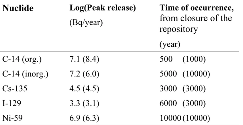
The breakthrough curves of the near-field releases are shown in figure 4.5 and the values of the peak releases in Table 4.2 (SKB results in parentheses). These results are for the maximum flow parameter.

Table 4.2 Peak release rates and their time of occurrence from 1BTF for the base case. The SKB results are in parentheses.

Nuclide Log(Peak release)

(Bq/year)

Time of occurrence,

from closure of the repository (year) C-14 (org.) 7.1 (8.4) 500 (1000) C-14 (inorg.) 7.2 (6.0) 5000 (10000) Cs-135 4.5 (4.5) 3000 (3000) I-129 3.3 (3.1) 6000 (3000) Ni-59 6.9 (6.3) 10000 (10000) 1 3 2 4 8 6 7 1 5 9 10

Figure 4.5a The release rate to the top filling of the 1BTF vault of organic C-14. The time scale starts when the repository is closed.

Time (yr) x10

R

el

ea

se

r

at

e

(B

q/

yr

)

_{C-14 (org.)}

Figure 4.5b The release rate to the top filling of the 1BTF vault of inorganic C-14 (inorg.) and Cs-135. The time scale starts when the repository is closed.

Time (yr) x 10

R

el

ea

se

r

at

e

(B

q/

yr

)

_{C-14 ( inorg.)}

Time (yr) x10

R

el

eas

e r

at

e (

B

q/

yr

)

Cs-135

Figure 4.5c The release rate to the top filling of the 1BTF vault of I-129 (upper) and of Ni-59 (lower). The time scale starts when the repository is closed.

Time (yr) x10

R

el

eas

e r

at

e (

B

q/

yr

)

_I-129

Time (yr) x10

R

el

ea

se

r

at

e

(B

q/

yr

)

_Ni-59

4.4 The BMA vault

4.4.1 Description of the barriers

The FEM model of the AD-equation together with the time dependent water flow used to estimate the releases of the BTF vaults (Equations 3.1 and 3.2) is used also for the BMA vault but with the geometry shown in figure 4.6 (see also figure 3.1). The degree of detail of this model is lower than that of 2BTF by disregarding the function of the drums, boxes etc. that contain the waste.

Initial conditions

The source term is given by a concentration C0 assuming that no walls separate the

different types of waste. The functioning barriers containing the initial concentration are therefore the bottom plate, the sidewalls of the vault and the top plate and top lid (figure

4.6). The original waste volume is 14400 m3 and the nuclides are assumed to be

homogeneously distributed in this volume.

The initial concentration for a given nuclide is therefore given by:

(

)

0 A/14400 Bq/m

C = (4.2)

where A is the initial inventory in Becquerel. Boundary conditions

The concentration is zero in the rock at a reasonable distance from the vault. Mass balance is established between the different regions using mixed boundary conditions. The integration domain is divided in twelve regions (figure 4.6).

Figure 4.6. The BMA vault divided into the regions defining the different barriers used in the FEM model.

7 1 3 4 6 2 5 8 9 10 11 12

The regions are:

- Zone 1 is a gap between the left lateral wall and the rock, which is filled with sand. - Zone 2 is the left lateral wall.

- Zone 3 is the right lateral wall.

- Zone 4 is the gap between the right lateral wall and the rock. It is also filled with sand.

- Zone 5 is a protection lid that will be poured over the top. - Zone 6 is a gap.

- Zone 7 is the top plate.

- Zone 8 is the top filling of sand and gravel. - Zone 9 is filled with gravel and sand. - Zone 10 is the bottom plate.

- Zone 11 is the interior of the vault (waste matrix).

- Zone 12 is a fracture connecting the waste to the top filling.

In the model the small gap between the top plate and the lid over it (zone 6) is disregarded because the water filling that gap does not offer any resistance to the nuclide migration. The main simplification of the model geometry is the fact that the nuclides are considered homogeneously spread in zone 11 and the boxes, drums etc. containing the different waste are not given any credit as barriers. Zone 9 (gravel and sand) has also been disregarded. The nuclides are assumed instantaneously dissolved in the water that penetrates the vault. Those nuclides will therefore penetrate the lateral walls, the roof and the lid plates due to diffusion and advection.

4.4.2 Results

The hydrogeological pattern around the BMA vault is the same as for the other regions of SFR 1, the groundwater flow being predominantly vertical and upwards during the first period of the repository history and changing gradually to an horizontal flow and finally to vertical flow downwards. In the calculation we assume conservatively a continuous vertical upward flow over the whole period; it is a conservative assumption because we “collect” the nuclides in the top filling (zone 8) during the whole time period.

The results of the near-field calculations are presented in figure 4.7 and the peak releases with their times of occurrence is shown in Table 4.3 (SKB’s results for intact barriers in parentheses). An illustration of the concentration of Ni-59 in the top filling is shown in figure 4.8.

Table 4.3 Peak release rates and their time of occurrence from BMA for the base case. The SKB’s results are in parentheses.

Nuclide Log(Peak release )

(Bq/year)

Time of occurence,

from closure of the repository (year) C-14 (org.) 7.6 (8.0) 900 (1500) C-14 (inorg.) 5.5 (5.5) 6000 (2000) Cs-135 4.4 (5.5) 10000 (2000) I-129 4.1 (4.1) 2000 (2000) Ni-59 8.6 (7.0) 10000 (10000)

Figure 4.7a Release rate of organic C-14 (upper) and of inorganic C-14 (lower) in Bq/year versus time in years. The time scale starts when the repository is closed.

R el ea se r at e (B q/ yr ) Time (yr) x103 C-14 (org.) Time (yr) x103 R el ea se r at e (B q/ yr ) C-14 (inorg.) L og r el ea se r at e (B q/ yr ) Time (yr) x103 Time (yr) x103 L og r el ea se r at e (B q/ yr )

Figure 4.7b Release rate of Cs-135 (upper) and I-129 (lower) in Bq/year versus time in years. The time scale starts when the repository is closed.

R el ea se r at e (B q/ yr ) Time (yr) x103 Cs-135 R el ea se r at e (B q/ yr ) Time (yr) x103 I-129 L og r el ea se r at e (Bq/ yr ) L og r el ea se r at e (Bq/ yr ) Time (yr) x103 Time (yr) x103

Figur 4.7c Release rate of Ni-59 in Bq/year versus time in years. The time scale starts when the repository is closed.

Figure 4.8 The concentration profile in the top filling of Ni-59 at 2000 years.

2000 yr R el ea se r at e (B q/ yr ) Time (yr) x103 Ni-59 L og r el ea se r at e (B q/ yr ) Time (yr) x103

4.5 The BLA vault

4.5.1 Description of the barriers

As for the study of the BMA vault simplifying assumptions on the geometry of BLA were needed due to restrictions imposed by the numerical FEM model. The waste inventory from sections with different waste types was averaged. Nevertheless this averaging procedure is sufficient for the aim of our study of the near-field releases. At relatively high water flow rates, the diffusion process as a transport mechanism is of minor importance. Therefore the assumed value of the effective diffusivity in the waste

matrix was given the same value of that in pure water (2.0×10-9 m2/s). The porosity of

the waste matrix is assumed to be 0.7 (Lindgren and Pers, 1991). The average specific flow is taken as the numerical mean of the lowest and highest value at each time point. The inventory is assumed to be immediately available to diffusion and advection because the waste forms are not effective as sorption barriers. The exception is the bottom plate (zone 5 in figure 4.9) for which sorption is considered. Zone 6 has been disregarded in the calculations.

Initial conditions

The source term C0 is obtained by averaging the total activity over the entire waste

volume, which gives:

3

0 (A/15100)Bq/m

C =

with A representing the total activity in Bq. Boundary conditions

The integration domain is show in figure 4.9. The mass balance in the interface between the barriers (regions) is assured by mixed type boundary conditions. The initial concen-tration of nuclides in the rock at a reasonable distance from the vault is assumed to be zero.

The regions are classified as: - Zone 1 is the top filling.

- Zone 2 is the gap between the waste matrix and the left wall. - Zone 3 is the waste matrix.

- Zone 4 is the gap between the waste matrix and the right wall. - Zone 5 is the concrete bottom plate.

- Zone 6 is made of gravel.

Figure 4.9. The BLA vault divided into the regions defining the different barriers used in the FEM model.

The Darcy flow used in these calculations is the numerical mean of the lowest and highest flow for each barrier (se Table 4, Appendix II). The reason for this choice is that the ratio between advective and dispersive/diffusive flow is such that the finite element code may not otherwise be stable when time increases.

4.5.2 Results

The nuclides are assumed to be instantaneously accessible to transport by the water in the vault. No advective flow is assumed through the waste matrix, the migration within the matrix being controlled by diffusion. The nuclides from the waste migrating into the top filling, into the lateral gaps between the waste packages and the side walls of the vault and into the gravel/sand filling under the bottom plate are transported by advection and diffusion. Because the walls of the containers are not functioning as barriers we have not considered the presence of any fractures as was the case for the other vaults. Table 4.4 shows peak releases and corresponding times.

Table 4.4 Peak release rates and their time of occurrence from BLA for the base case. The SKB results are in parentheses.

Nuclide Log(Peak release )

(Bq/year)

Time of occurence,

from closure of the repository (year) C-14 (org.) 4.1 (4.5) 200 (1000) C-14 (inorg.) 7.2 (7.5) 200 (1000) Cs-135 4.3 (4.4) 500 (1000) I-129 3.0 (3.2) 200 (1200) 4 1 2 2 6 5 1 3 7

Figure 4.10a Near-field release rates from BLA of C-14 organic and inorganic (upper and lower pictures respectively). The time scale starts when the repository is closed.

Time (yr) x103 R el ea se ra te ( Bq /y r) C-14 (org.)

L

og

r

el

ea

se

r

at

e

(B

q/

yr

)

Time (yr) x10

Figure 4.10b Near-field release rates from BLA of Cs-135 (upper) and I-129 (lower). The time scale starts when the repository is closed.

Time (yr) x 103 R el ea se r at e (B q/ yr ) Cs-135 Time (yr) x103 L og r el ea se r at e (B q/ yr ) L og r el ea se r at e (B q/ yr ) I-129 Time (yr) x103

Figure 4.10c Near-field release rates from BLA of Ni-59. The time scale starts when the repository is closed. L og r el ea se r at e (Bq/ yr ) Time (yr) x103 Ni-59

5. Complexing agents

The influence of complexing agents, keeping the barriers intact as in the base case, is accounted for by a decrease of the retention capacity of those barriers. This is

represen-ted by lowering the Kd values by a factor of ten (Table 2-5 and tables of Appendix II).

The rest of the data are the same as in the base case. Of the nuclides analysed in the previous cases only Ni-59 is considered by SKB and is therefore the only one con-sidered in this Chapter.

5.1 2BTF

The release of nickel to the near-field is shown by figure 5.1. It is observed that the release rate at 10000 years, is one order of magnitude higher than for the base case where there is no influence from complexing agents (figure 4.3). The difference is higher at early time points as expected. The breakthrough curve in figure 5.1 increases and then declines slowly (wash out effect of the radionuclide) in contrast with the case of the absence of complexes where the curve rises all the time and does not peak within the first 10000 years.

Figure 5.1 The 2BTF breakthrough curve of Ni-59 for the case of complexing agents. The time scale starts when the repository is closed.

Ni-59 Time (yr) x 103 R elea se r at e (B q/yr ) L og r el ea se r at e (B q/ yr )

5.2 1BTF

In this case the release rate of the Ni-59 escaping from the vault increases all the time as shown by the breakthrough curve of figure 5.2. It does not peak before the first 6000 years as was also the case when no complexing agents were present. We used here a simulation cut-off of 6000 years because the model becomes numerically unstable after that time. The highest differences between two cases are found during the first 2000 years.

Figure 5.2 The 1BTF breakthrough curve of Ni-59 for the case of complexing agents. The time scale starts when the repository is closed.

Rel

eas

e rat

e

(Bq

/y

r)

Ni-59

3

5.3 BMA

Ni-59 migration in the near-field is in this case described by the curve shown in figure 5.3. Between 4000 years and 10000 years the release rate is almost equal to that of the base case. The presence of complexes affects mainly the early releases.

Figure 5.3 The BMA breakthrough curve of Ni-59 for the case of complexing agents. The time scale starts when the repository is closed.

Time (yr) x10

R

el

ea

se

r

at

e

(B

q/

yr

)

_Ni-59

Ni-59

5.4 BLA

The peak release is almost equal to that of the base case but the amount of Ni-59 decreases more rapidly in this case because of the nil sorption in the barriers of the vault. A cut-off of 6000 years for the calculations has been chosen because after 5000 years the releases are small and the numerical code becomes unstable as can be seen in the figure.

Figure 5.4 The BLA breakthrough curve of Ni-59 for the case of complexing agents. The time scale starts when the repository is closed.

Time (yr) x10

3

R

el

ea

se

r

at

e

(B

q/

yr

)

Ni-59

Ni-59

6. Variability studies

6.1 The impact of fractures on the radionuclide release

In the base case studies we assumed the existence of a fracture in the 2BTF concrete barriers connecting partially the waste with the top filling. To estimate the dependence of the release rate on the existence of a fracture (the same fracture as in the base case), two calculation cases with and without the fracture are performed. The input data of the base case is used with the exception of the Darcy flow. The results for inorganic C-14 using the minimum Darcy flow are shown in figure 6.1. The use of the minimum value is due to numerical instabilities that do not allow higher values.

Figure 6.1 The release of inorganic C-14 to the top filling of the 2BTF vault with and without a fracture (left and right respectively). The time scale starts when the repository is closed.

It is seen that the existence of the fracture increases the peak release rate by a half order of magnitude. The difference is higher at early time points.

6.2 The impact of the Darcy flow on the radionuclide release

To investigate the dependence the Darcy flow has on the release rate, two calculation cases are performed for the minimum and maximum Darcy flow used by SKB. The first case treats the migration of Ni-59 from the BMA repository and the second one the migration of inorganic C-14 from the 2BTF repository. In both cases a fracture is

present in the concrete barriers. Except for the variation of the Darcy flow parameter the input data used is that of the base case.

The result of the first variation is shown in figure 6.2. The two breakthrough curves are similar but with peak releases differing in by one-half order of magnitude. The result of

Time (yr) x10

R

el

ea

se

r

at

e

(B

q/

yr

)

_{C-14 (inorg.)}

Time (yr) x10

R

el

ea

se

r

at

e

(B

q/

yr

)

_{C-14 (inorg.)}

Time (yr) x103 _{Time (yr) x10}3

C-14 (inorg.)

C-14 (inorg.)

the second variation is shown in figure 6.3. The two breakthrough curves are for most time points very close to each other.

Figure 6.2 The variation of the release of Ni-59 from the BMA vault due to the

variation of the Darcy flow. The left picture is calculated with all barriers of the BMA assuming the respective maximum Darcy flow. The picture at right is for the minimum Darcy flow. The time scale starts when the repository is closed.

Figure 6.3 The release of inorganic C-14 to the top filling of the 2BTF vault for the lowest (left) and highest (right) Darcy velocity values for each barrier. The time scale starts when the repository is closed.

Time (yr) x103 R el ea se r at e (B q/ yr ) Ni-59

Fig 6-2

6.3 The impact of a large fracture in the concrete barriers

In this section we address some variability studies connected with the degradation of barriers over time. We assume that one fracture will develop in such a way that it connects the bottom floor to the roof of the vaults (the top filling). This is illustrated for the case of the 2BTF vault by figure 6.4. The same dimensions and geometry of that fracture is used for the other vaults, 1BTF and BMA.

Figure 6.4 The 2BTF vault with a fracture connecting the floor to the top filling. The case studies is conducted for five radionuclides, organic and inorganic C-14, Cs-135, I-129 and Ni-59. Apart from the new data required for the fracture region, we use data of the corresponding base case. The fracture makes in all cases an angle of 45˚ with the floor and it is 3.5 cm wide. For the sake of simplicity we assume that the fracture is present at the time when the repository is closed. The Darcy velocity in the fracture varies continuously from the value used for the bottom plate to the value used for the top filling.

6.3.1 2BTF results

The results are shown in figure 6.5. It is observed that the breakthrough curves do not differ substantially from those given in the base case (se figure 4.2).

Figure 6.5a Release rate of C-14 from the 2BTF vault with a large fracture connecting the floor to the top filling. The time scale starts when the repository is closed.

C-14 (org.)

Time (yr) x10

R

el

ea

se

r

at

e

(B

q/

yr

)

C-14 (org.)

C-14 (inorg.)

R

el

ea

se

r

at

e

(B

q/

yr

)

Time (yr) x10

C-14 (inorg.)

Figure 6.5b Release rate of Cs-135 and I-129 from the 2BTF vault with a large fracture connecting the floor to the top filling. The time scale starts when the repository is closed.

R

el

ea

se

r

at

e

(B

q/

yr

)

Time (yr) x10

Cs-135

Cs-135

Time (yr) x10

R

el

ea

se

r

at

e

(B

q/

yr

)

I-129

I-129

Figure 6.5c Release rate of Ni-59 from the 2BTF vault with a large fracture connecting the floor to the top filling. The time scale starts when the repository is closed.

The picture below illustrates an asymmetric concentration profile of the radionuclide I-129 released to the top filling of the 2BTF in the presence of the large fracture.

Figure 6.6 The concentration of I-129 in the top filling is higher at the outlet of the large fracture.

Ni-59

Time (yr) x10

R

el

ea

se

r

at

e

(B

q/

yr

)

Ni-59

Figure 6.7 shows the concentration profile of Cs-135 in a cross section of the 2BTF vault.

6.3.2 1BTF results

The 1BTF results are shown in figure 6.8. The breakthrough curves of inorganic C-14 differ by roughly one order of magnitude compared to the base case (see figure 4.5). The releases of the other nuclides are not so influenced by the presence of the large fracture.

Figure 6.8a Release rate of C-14 (inorganic and organic) from the 1BTF vault with a large fracture connecting the floor to the top filling. The time scale starts when the repository is closed.

Time (yr) x10

R

el

ea

se

r

at

e

(B

q/

yr

)

C-14 (inorg.)

C-14 (inorg.)

C-14 (org.)

Time (yr) x10

R

el

ea

se

r

at

e

(B

q/

yr

)

C-14 (org.)

Figure 6.8b Release rate of I-129 and Cs-135 from the 1BTF vault with a large fracture connecting the floor to the top filling. The time scale starts when the repository is closed.

R

el

ea

se

r

at

e

(B

q/

yr

)

Time (yr) x10

3

I-129

_I-129

Cs-135

Time (yr) x10

3

R

el

ea

se

r

at

e

(B

q/

yr

)

Cs-135

Figure 6.8c Release rate of Ni-59 from the 1BTF vault with a large fracture connecting the floor to the top filling. The time scale starts when the repository is closed.

6.3.3 BMA results

The results are shown in figure 6.9. It is observed that the breakthrough curves do not differ substantially from those given by vaults without the large fracture (see figure 4.7).

Figure 6.9a Release rate of C-14 (inorg.) from the BMA vault with a large fracture connecting the floor to the top filling. The time scale starts when the repository is

Ni-59

Time (yr) x10

R

el

ea

se

r

at

e

(B

q/

yr

)

Ni-59

R

el

ea

se

r

at

e

(B

q/

yr

)

Time (yr) x10

C-14 (inorg.)

_{C-14 (inorg.)}

Figure 6.9b Release rate of C-14 (org.) and Cs-135 from the BMA vault with a large fracture connecting the floor to the top filling. The time scale starts when the repository is closed.

Time (yr) x10

Cs-135

R

el

ea

se

r

at

e

(B

q/

yr

)

Cs-135

R

el

ea

se

r

at

e

(B

q/

yr

)

Time (yr) x10

C-14 (org.)

C-14 (org.)

Figure 6.9c Release rate of I-129 and Ni-59 from the BMA vault with a large fracture connecting the floor to the top filling. The time scale starts when the repository is closed.

I-129

Time (yr) x10

R

el

ea

se

r

at

e

(B

q/

yr

)

I-129

Ni-59

7. Summary and conclusions

In this work we develop four two-dimensional models of the SFR 1 vaults (1BTF, 2BTF, BMA and BLA) and apply them to calculate the near-field release rates for some representative nuclides. To translate the models to numerical codes we use the approach of finite elements (FEM).

The vaults are modelled as 2D sections perpendicular to the longitudinal axis of the vaults. The transport of radionuclides is dominated by advection and diffusion through the different barriers that isolate the waste and by retardation of the nuclides in those barriers.

Our results may be somewhat conservative because we use the maximum value of the vertical Darcy flow for all barriers in all vaults except for BLA vault where we use the mean value. Having this in mind the results are in reasonable agreement with the results of Lindgren et.al., October 2001. The differences may illustrate the impact of concep-tual uncertainties associated with the difference in the model approach used in this report and by SKB. The main processes are represented in both models; advection, dispersion/diffusion, retardation and radioactive decay. The difference is in the geometry. In fact, the “block” approach of the SKB model is quite different from our approach where we tried to have a more realistic representation of the geometry of the repository (in two-dimensions).

In the framework of deterministic calculations the conceptual uncertainty cannot be properly assessed due to the fact that it would required a huge number of calculations with different parameter combinations which would make the exercise intractable and one would loose in transparency. On the other hand it is not possible at present to make probabilistic calculations using FEM models because of the simulation time for each calculation is too long which is a clear disadvantage with our model approach. The main advantage is that we get a reasonably transparent representation in the modelling and in the introduced assumptions by using the AD equations directly applied to the geometry of the vaults.

A desirable feature to improve our present representation of the SFR 1 would be to connect a model of the SFR 1 Silo to the four vault models developed here into a single framework making it possible to assess the entire repository as a whole.