Processing of full waveform sonic data for shear wave velocity at the Ketzin CO2 storage site

(1)

Examensarbete 30 hp

May 2009

Processing of full waveform sonic data for shear wave

velocity at the Ketzin CO

2

storage site

(2)

ABSTRACT

The accumulation of carbon dioxide gas (CO2) in the atmosphere is considered be the main cause

of global warming effects. These emissions can be reduced substantially by capturing and storing the CO2. The CO2SINK project started in April 2004 in the northeast German Basin (NEGB) at

the town of Ketzin near Berlin, Germany. Uppsala University is one of the main participants in the seismic part of the CO2SINK project.

Full waveform sonic data were acquired in the Ktzi-201 injection well at the Ketzin CO2 storage

site. The mode of logging was monopole logging. The target was the Stuttgart Formation, a saline sandstone aquifer at the depth of 500-700m. A total of 1210 shots were conducted and data were recorded on 13 channels. Receiver spacing was 6 inches (15.24 cm).

The focus of the CO2SINK project was to develop the basis for the CCS technique by injecting

CO2 into a saline aquifer and monitoring of the injected CO2 in the aquifer as a pilot study for

future geological storage of CO2 in Europe.

The objective of this study is to calculate P-wave & S-wave velocities from full waveform sonic data recorded in Ktzi-201 injection well. In hard formations, shear wave velocities can be determined directly from full waveform sonic data recorded in monopole logging. However, in slow formations like Stuttgart Formation as in the Ketzin CO2SINK project, shear wave arrivals

are absent in full waveform sonic data recorded in monopole logging. In this case, shear wave velocities can be determined from Stoneley wave velocities provided that one knows the P-wave velocity in the borehole fluid.

P-wave velocities were calculated by picking the P-wave arrivals on full waveform sonic data. Due to the absence of shear wave arrivals, the shear wave velocities were estimated from the larger amplitude Stoneley waves. The estimated S-wave velocities from Stoneley waves were less than the fluid wave velocity in the borehole, confirming the mode of logging was monopole and the formation is a slow formation.

The reliability of shear wave velocities estimated from Stoneley waves also depends on five other parameters such as formation permeability, borehole fluid property, tool diameter, borehole radius etc.

(3)

Acknowledgement

Studying abroad is my big dream which come true. It is an unexpected and incredible experience which is full of challenges along the journey. A milestone of this nature could never be possible to achieve without the support of a galaxy of some truly loving persons. No words to describe my feelings of respect about my affectionate parents and whose love, encouragement and prayers invariably buoyed me up. Their concern, devotion and love can never be paid back. I have no words to say thanks to these all. I cannot forget the love and patient of my whole family during my academic careers.

I owe my deepest gratitude to my supervisor, Prof. Christopher Juhlin, for giving me the opportunity to work with him and giving me an initiative to this study and guided me with his valuable suggestions. His encouragement, guidance, positive criticism, sympathetic attitude and sincere cooperation were vital for the completion of this thesis. I pay special gratitude to admirable personality Sayed Hesammoddin Kazemeini. His guidance and support was crucial for completion of this thesis work.

I pay my thanks to whole faculty of the reflection and refraction seismic group at the Department of Earth Science, Uppsala University especially the teachers whose valuable knowledge, assistance, cooperation and guidance enabled me to take initiative, develop and furnish my academic carrier. I acknowledge GLOBE ClaritasTM under license from the Institute of Geological and Nuclear Sciences Limited, Lower Hutt, New Zealand, which was used to process the seismic data.

I have been fortunate to have a very nice company of friends especially Nauman, Noor, Kamran, Wahab, Abrar and others offering enjoyable moments and making from every day a special and different day during my stay in Uppsala.

Last but not least, I would like to thank Dr. Aamir Ali for his moral support and encouragement for writing this thesis.

Khalid Abbas, Uppsala, May, 2009

(5)

1. Introduction

The accumulation of carbon dioxide gas (CO2) in the atmosphere is considered to be the main

cause of global warming effects. This accumulation is a result of the extensive burning of fossil fuels that began during the Industrial Revolution. Approximately one third of all CO2 emissions

due to human activity come from fossil fuels used for generating electricity. A variety of other industrial processes also emit large amounts of CO2, for example oil refineries, cement works,

and iron and steel production (IPCC, 2005). These emissions could be reduced substantially by capturing and storing the CO2.

Carbon dioxide (CO2) capture and storage (CCS) is a process consisting of the separation of CO2

from its sources, transport to a storage location and long-term isolation from the atmosphere. CCS has the potential to reduce overall mitigation costs and increase flexibility in achieving greenhouse gas emission reductions. CO2 capture can be done at large point sources and then be

compressed and transported for storage in geological formations, in ocean, in mineral carbonates, or for use in industrial processes (IPCC, 2005).

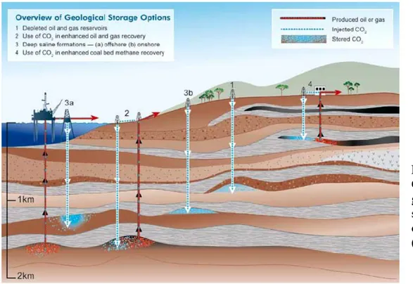
Storage of CO2 in deep, onshore or offshore geological formations uses many of the same

technologies that have been developed by the oil and gas industry. These technologies have been proved to be economical feasible under specific conditions for oil and gas field and saline formations. If CO2 is injected at depth below 800m into suitable saline formations or oil and gas

fields, various trapping mechanisms would prevent it from migrating to the surface. Generally, a caprock provides the same purpose. Coal bed storage may take place at shallower depths and mainly relies on the absorption of CO2 in the coal. CO2 storage can also be used with Enhanced

Oil Recovery (EOR) as shown in figure 1 (IPCC, 2005).

Figure 1. Overview of geological storage options (IPCC, 2005)

(6)

A brief overview of an ongoing large project for CO2 capture and storage is given below:

1.1 The Sleipner Project:

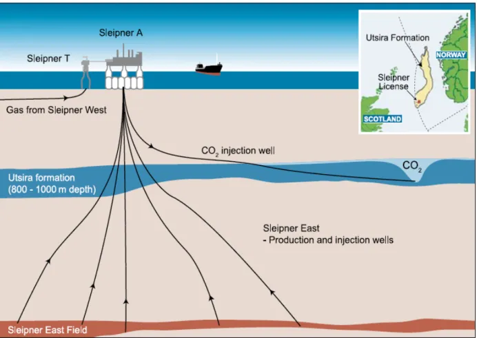
The Sleipner project is believed to be the world’s first industrial scale CO2 storage operation that

has been operated in Sleipner field in North Sea since 1996. CO2 is being injected into Utsira

Sand, a major regional saline aquifer at a depth of 1000m shown in Figure 2. The projected final target of injection is about 20 Mt. The Sleipner sequestration operation is the focal of Saline Aquifer CO2 Storage (SACS) and its aims are monitoring and modeling the injected CO2 and

regional characterization of Utsira reservoir and its caprock (Chadwick et al., 2004). The CO2

capture takes place directly at the Sleipner T (Treatment) platform where it is also compressed. About one million tons of CO2 per year (nearly 3 per cent of Norwegian CO2 emissions in 1990)

have been injected since October 1996 in Statoil’s Sleipner CO2 Storage Project (IEA, 2004).

Figure 2. Simplified diagram of the Sleipner CO2 Storage Project. Inset: location and extent of

the Utsira formation (IPCC, 2005).

1.2 The CO2SINK PROJECT

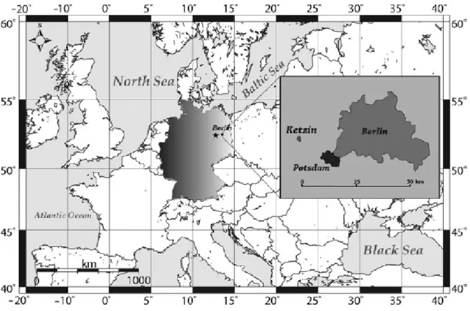
CO2SINK project, the first European research and development project, related to the in-situ

(7)

CO2 into a geological formation in the northeast German Basin (NEGB) at the town of Ketzin

near Berlin Germany as shown in figure 3.

Figure 3. Location of Ketzin CO2 injection site (Kazemeini et al., 2009).

The Ketzin gas storage site was selected for CO2SINK project because of following reasons

(Juhlin et al., 2007):

• Industrial land and infrastructure of Ketzin site makes it suitable for a small scale demonstration of CO2 injection and storage.

• The anticline at Ketzin was used for gas storage in the past. Natural gas methane was stored until the year 2000 at Ketzin site in Jurassic sandstones at depth of 250-400m. The site was abandoned in 2004 but infrastructure is still there.

• These sandstones with interlayered mudstones, siltstone and anhydrite form a shallow multiaquifer system.

In the Ketzin CO2SINK project, special attention should be given to the monitoring of geological

storage. Answers to important questions will be addressed in this project. Can migration of CO2

within the reservoir, through boreholes and leakage via faults be mapped? Monitoring the quality of geological seals, the reservoir itself and changes as CO2 is being injected and dissolves in

(8)

Three boreholes, one injection borehole and two observation boreholes were drilled into the flank of the Ketzin anticline with a spacing of about 50-100m as shown in figure 4. The boreholes were drilled according to plan in 2007 (Forster et al., 2008).

Figure 4. Aerial view of CO2SINK drilling site showing injection well (CO2 Ktzi 201/2007) and

observation well #2 (CO2 Ktzi 202/2007), Observation well #1 (CO2 Ktzi 200/207). CO2 storage

tanks with the pump house are also visible (Prevedel et al., 2008).

Uppsala University is one of the main participants in the seismic part of the CO2SINK project.

Seismic monitoring is an important part of the CO2SINK project and includes cross-well, vertical

seismic profile (VSP), moving source profiling and 2D and 3D time-lapse techniques. To determine the favorable acquisition parameters, a pilot seismic study was carried out in 2004. A 3D baseline seismic survey with 12km2 of sub-surface coverage was acquired in 2005. Clear E-W trending faults on the crest of the Ketzin anticline can be seen in the 3D survey which also showed a clear signature from remnant gas in sandy Jurassic formations (Kazemeini et al., 2009). During the fall of 2007, borehole baseline seismic data were acquired, both vertical seismic profiling (VSP) and moving source profiling (MSP). Borehole geophysical logs have also been acquired for seismic monitoring of the CO2SINK project.

(9)

The injection of CO2 started on June 30th 2008 and up to May 3rd 2009, 14.073 tons of CO2 had

been injected in the underground.

1.3 Objectives of this study:

The objective of this study is to estimate P-wave velocities and compare those velocities with already provided velocities by Schlumberger.

In slow formations like Stuttgart Formation as in the Ketzin CO2SINK project, shear wave

arrivals are absent in full waveform sonic data recorded in monopole logging. In this case, shear wave velocities can be determined from Stoneley wave velocities, provided that one knows the P-wave velocity in the borehole fluid. This project work focuses on obtaining better estimates for shear wave velocity from larger amplitude Stoneley wave.

(10)

2. Geological Setting

The CO2SINK project is aimed at a pilot CO2 storage in a gentle anticline in the northeast

German Basin (NEGB) which is part of a Permian basin system. This Permian basin system extends from the southern North Sea to Poland. In the early Permian, the basin origin started with initial rifting. Subsidence followed the rifting which resulted in the deposition of Permian clastic rocks and the Upper Permian Zechstein salt. In the late Permian, a phase of accelerated subsidence started followed by relatively low subsidence rate from middle Triassic to early Jurassic (Juhlin et al., 2007). In the Triassic, Jurassic, and early Cretaceous, major rift- and wrench tectonics took place. This renewed tectonic activity resulted in the formation of local north-northeast - south-southwest directed depocenters in the NEGB. Throughout the late Cretaceous and Paleocence, the NEGB remained mainly metastable with only some local highs and marginal troughs developing (Juhlin et al., 2007).

The Ketzin site is located in the eastern part of a double anticline which formed above an elongated salt pillow situated at a depth of 1500-2000m. The axis of the anticline strikes north-northeast - south-southwest and its flanks gently dip about 15’o’ (Forster et al., 2006). Geologic formations of the Triassic (Buntsandstein, Muschelkalk, and Keuper) and Lower Jurassic form the immediate overburden above the salt pillow. Stratigraphic succession shows a first gentle uplift of the Ketzin anticline started in Early Triassic. About 140Ma ago, major uplift occurred which resulted in erosion of Lower Jurassic (Toarcian) and the Middle and Upper Jurassic formations. A second uplift occurred at 106Ma which resulted in the erosion of the previously deposited Lower Cretaceous. The total amount of eroded thickness is about 500 m (Forster et al., 2006). The Upper Cretaceous probably was never deposited in the area, which at that time was part of a structural high. Sediments of the Oligocene (Rupelton) form the first formation unaffected by anticlinal uplift resting above Jurassic sediments and these sediments are the first indicators of regional downwarping of central parts of NEGB which lasted until present (Forster et al.,2006).

Natural gas had earlier been stored at the site from the 1970s until 2000 at depths of 250 m to 400 m in Jurassic sandy layers sealed with a thick layer of Rupelian clay and interbedded mudstone (Kazemeini et al., 2009). However, the target reservoir in the CO2SINK project at the

injection site is a deeper saline aquifer within the upper Stuttgart Formation of Triassic age, at a depth of 625 to 700m as shown in Figure 5 (Kazemeini et al., 2009; Forster et al., 2006).

The Stuttgart Formation contains heterogeneous lithology and is of fluvial origin (Forster et al., 2008). Sandy channel-facies rocks (good reservoir properties) deposits alternate with muddy, flood-plain facies rocks (poor reservoir quality). The sandstone interval may attain thickness from 1m to 30m where subchannels are stacked. The width of a fluvial channel-string system is from several tens of meters to several hundreds of meters (Forster et al., 2006).

(11)

Figure 5. Geology of the Ketzin anticline for selected boreholes including the injection well CO2

Ktzi 201/2007 with aquifer (light yellow) and acquitard (pink) (Forster et al., 2008).

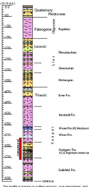
The Weser and Arnstadt formations consisting of mudstones form an approximately 200 m thick cap rock above the Stuttgart Formation. Additional aquifer-aquitard systems are present further up, at 250m to 400m depth, in the form of Jurassic sandstone interbedded with mudstone, claystone and siltstone that form a multi aquifer system. The thickness of tertiary clay acting as caprock is from 80-90m, which covers the Jurassic sandstones. This clay plays an important role in separation of non-saline groundwater in shallow Quaternay aquifers from saline waters in the deeper aquifer. Local erosion of the Rupelton aquitard at some locations results in ascending saline waters that mix with the fresh waters of the shallow aquifers (Kazemeini et al., 2009). The stratigraphic column based on well CO2 Ktzi 200/2007 is shown in figure 6.

(12)

Figure 6. Stratigraphy of the Ketzin structure based on a geological profile of the CO2 Ktzi

(13)

3. Review of Acoustic Logging Method

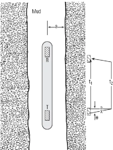
Acoustic logging is one of the principal geophysical well logging disciplines. As formation acoustic properties (velocity and attenuation), are closely related to rock type and formation fluid such as hydrocarbons, measuring these properties can provide useful information for formation evaluation. A tool is lowered into the borehole in acoustic logging and an acoustic or sound wave is generated by a transmitter or source in the tool. The sound wave travels along the borehole and interacts with the formation (Tang et al., 2004).

The receiver picks up and records the pulse as it arrives at the receiver. The sonic log is simply a recording versus depth of time, t, required for a sound wave to traverse 1ft of formation as shown in figure 7. Interval transit time Δt or slowness, is the reciprocal of velocity of the sound wave which depends upon formation lithology and porosity. That’s why sonic logs are very useful as porosity logs (Schlumberger, 1989). The tool is pulled up or lowered by wireline cable and the measurement is made continuously along the borehole. The wireline cable supplies power from, and transmits data to, a surface control system. Such type of logging is called Wireline logging. The output of acoustic logging is an acoustic log of acoustic properties of the formation around the borehole (Tang et al., 2004).

Figure 7. A borehole device for

measuring the interval transit time Δt. Ray paths of the acoustic energy refracted from the borehole into formation and back to the receiver are shown to the side (Ellis et al., 2008).

(14)

The conventional approach of acoustic logging can be used to measure the velocities of compressional and shear waves (with dipole tool) which can be further related to formation porosity and lithology. Abnormal high pore pressures and mechanical rock properties & fractures are also possible to infer and estimate from acoustic measurements (Ellis et al., 2008).

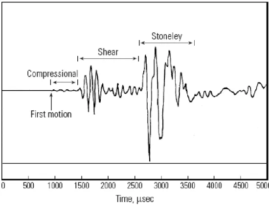
The acoustic waveform recorded with a logging device in a borehole shows the following distinct packets of energy.

3.1 Body waves:

3.1.1 Compressional waves:

Compressional waves are also called P-waves or longitudinal waves in which particle motion is co-linear with direction of propagation. These waves travel faster than shear waves and are recorded first on waveform data as shown in figure 8.

3.1.2 Shear waves:

Shear waves are also called S-waves or transverse waves in which particle motion is perpendicular to the direction of propagation (Boyer et al., 1997).

(15)

3.2 Interface waves:

3.2.1 Pseudo-Rayleigh waves:

Pseudo-Rayleigh waves are reflected conical dispersive waves (Biot, 1952). Their phase and group velocities approach the S wave velocity of the formation at low frequency (<5kHz) while at high frequencies (>25kHz) their velocity becomes asymptotic to the compressional wave velocity of the fluid. It is only encountered in fast formations (Boyer et al., 1997).

3.2.2 Stoneley waves:

Stoneley waves are of large amplitude that have traveled from transmitter to receiver with a velocity less than that of the compressional wave in the borehole fluid (Boyer et al., 1997). The Stoneley wave has a lower sensitivity to the formation shear velocity and it is strongly influenced by other factors such as frequency of sound pulse, formation permeability, borehole fluid property, tool diameter, borehole radius etc, (Tang and Cheng, 1993). Stoneley waves are similar to the tube waves observed in VSP.

3.2.3 Fluid waves:

Fluid waves are guided (or channel) waves, having very little scattering and they propagate through the fluid of the borehole (Boyer et al., 1997).

The waveform will contain P- and S-waves in the case of a Fast formation where shear velocity exceeds the sound velocity of the borehole fluid. In the case of slow formation, where shear velocity of the formation is less than the sound velocity of the fluid in borehole, borehole acoustic logging waveform data will consist of a compressional head wave, a direct (fluid) compressional wave of low amplitude, and a late arriving, low frequency Stoneley wave (Stevens and Day, 1986).

3.3 Types of Tools: 3.3.1 Monopole tools

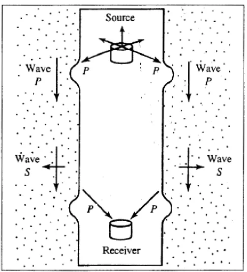
Monopole sonic logging tool has an axial symmetry and is equipped with multidirectional receivers as shown in figure 9.

A compressional wave is generated in fluid by transmitter in every direction, producing a P-wave and a S-wave in the surrounding formation at the critical angles of refraction (Boyer et al., 1997). In a vertical well, the monopole tool can be used to record five types of waves:

(16)

2) refracted S-waves, only in fast formations 3) fluid waves

4) two dispersed tube waves, i.e. pseudo-Rayleigh and Stoneley waves (Mari et al., 1994).

Figure 9. Monopole tool showing generation of P- and S-waves (Boyer et al., 1997).

In monopole logging, borehole acoustic logging waveforms consist largely of two guided wave modes: the Stoneley and pseudo-Rayleigh waves (Toksoz and Cheng, 1981).

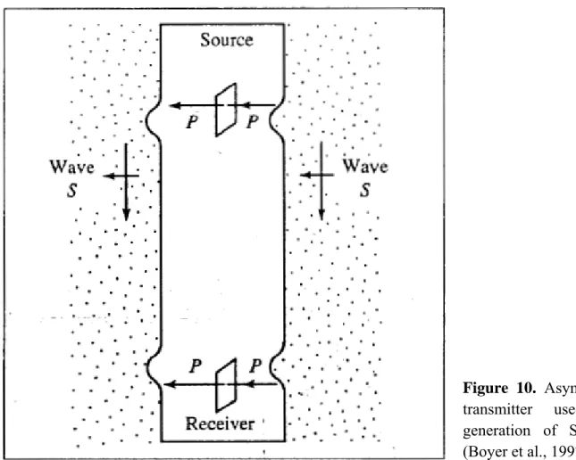
3.3.2 Dipole Tools

A dipole tool is shown in figure 10. This tool is useful in determining the S-wave velocity in slow formations (when S-wave velocity in formation is less than P-velocity in mud). In a dipole tool, sources and receivers are polarized. The emitted P-wave is polarized perpendicular to the well which generates pseudo S-waves which propagate in a parallel direction to the well (Mari et al., 1994).

(17)

Figure 10. Asymmetric

transmitter used for generation of S-waves (Boyer et al., 1997).

3.4 Estimation of S-wave velocity using other types of waves 3.4 Estimation of S-wave velocity using other types of waves

The waveform may consist of two main body waves propagating in a fluid-filled borehole: the P- and S-waves as in the case of Fast formations. In case of slow formations, borehole acoustic logging waveform will consist of compressional head wave, a direct (fluid) compressional wave of low amplitude, and a late arriving, low frequency Stoneley wave (Stevens and Day, 1986). This was the case in the Ktzi-201 injection well as show in figure 11. Here the P-wave and the Stoneley wave can be easily seen, but the S-wave arrivals are absent.

In this situation, the shear wave velocity can be measured from Stoneley waves recorded by a monopole tool (Cheng et al., 1983, Stevens and Day, 1986). The absence of a critical refraction means that no shear waves can be measured directly in monopole logging (Tang et al., 1995). In this situation, the shear wave velocity can be measured from Stoneley waves recorded by a monopole tool (Cheng et al., 1983, Stevens and Day, 1986). The absence of a critical refraction means that no shear waves can be measured directly in monopole logging (Tang et al., 1995). 2 s 2 f s f f V V 1 V C ρ ρ + = (1)

(18)

Figure 11. Screen dump of Shot ID 1 showing the P-wave and the Stoneley wave.

Borehole fluid properties Vf and ρf can be measured or estimated from the type of drilling fluid

used (Tang et al., 1995).

The next unknown parameter in equation (1) was the borehole fluid velocity Vf. Unfortunately;

no measurement of borehole fluid velocity (Vf) was available at Ktzi-201. If we know the

composition of the borehole mud and temperature & pressure, we can calculate the velocity of fluid (Batzle et al., 1992). In this case, the velocity of borehole mud (Vmud) will be same as the

borehole fluid velocity (Vf). The constituents of borehole mud was mainly bentonite Be (4%)

and brine water Br (96%). A simple polynomial in temperature (T), pressure (P) and salinity (S) is made to calculate the density of the brine (ρBr) (Batzle et al., 1992).

ρw = 1+10-6(-80T–3.3T2+0.00175T2+489P-2TP+0.016T2P–1.3×10-5T2P–0.333P2 – 0.002TP2),

(2) ρBr = ρw + S{0.668+0.44S+10-6[300P – 2400PS + T(80 + 3T – 3300S – 13P + 47PS)]}, (3)

where ρw is the density of the water and S is the weight fraction (ppm/1000000) of sodium chloride.

(19)

The relationship for the velocity Vw of pure water to 1000C and about 100MPa is: j i i j ij w w T P V

∑∑

= = = 4 0 3 0 , (4)

where the coefficients of wij are given by Batzle et al., (1992).

Br Br Br K V ρ = , (5)

Where KBr is the bulk modulus of water and ρBr is the density of brine in g/cm3.

The equation for Vmud is given below (Poletto et al., 2002):

mud mud mud K V ρ = , (6)

Where Kmud is the bulk modulus of the mud and ρmud is the density of brine in g/cm3.

All the parameters in equation (1) are known except Vs, which can be easily calculated.

3.5 Dataset used for this study:

The full waveform sonic data in borehole Ktzi-201 (Injection well) was acquired in July, 2007. The mode of logging was monopole logging. The target was the Stuttgart Formation, saline sandstone aquifer. A total of 1210 shots were conducted and data were recorded on 13 channels. Receiver spacing was 6 inches (15.24 cm).

3.6 Software used for this study:

The data processing was done in GLOBE Claritas on a LINUX computer. In order to avoid the introduction of artifacts into processed volumes, the processing algorithm was kept simple Screen dumps of workflows and picking of wave arrivals in GLOBE Claritas are shown in Appendix A. MATLAB is used to calculate velocities and Microsoft Excel is used for plotting of velocities along depth of the borehole.

(20)

4. Results & Discussion:

A Full waveform sonic data were acquired in the Ktzi-201 injection well at the Ketzin CO2

storage site. The mode of logging was monopole logging. The objective was to pick P-wave & S-wave arrivals on full S-waveform data and calculate P-S-wave & S-S-wave velocities. On approximately all shots, P-wave was apparent and was easy to pick as shown in Appendix - A. One example of picking of P-wave arrivals at Shot ID 120 is shown in figure 12.

Figure 12. shows the waveform recorded at shot ID 120 and P-wave can be seen and easily

picked.

These picked times of the P-wave arrivals were plotted in MATLAB as a function of distance to calculate wave velocities. A best fit line is made and the slope of the best fit line gives us P-wave velocity on that shot.

Once all the velocities of the P-wave on all shots were calculated, these P-wave velocities were plotted against depth in the Ktzi-201well as shown in figure 13.

(21)

Figure 13. Calculated P-wave velocities are plotted against borehole depth to produce a Vp log

The calculated P-wave velocities were then compared with Schlumberger’s provided P-wave velocities as shown in figure 14.

(22)

Figure 14. Comparison of calculated P-wave velocities with Schlumberger’s provided P-wave

velocities.

After the P-wave calculation, our objective was to pick S-wave times to calculate S-wave velocities, but S-waves were absent on the full waveform sonic data of Ktzi-201.

(23)

The monopole logging method was used in Ktzi-201 well and in the monopole logging method, no shear waves can be measured directly in monopole logging. According to equation (1), shear wave can be calculated from Stoneley wave.

As the Stoneley wave has larger amplitudes, it is easy to pick on the full waveform sonic data of Ktzi-201 well. Figure 15 shows the Stoneley wave pick on Shot ID 100.

Figure 15. showing pick of Stoneley wave on Shot ID 100.

The Stoneley wave picked times were plotted as a function of distance in MATLAB and a best fit line is made. The slope of the line gives us the velocity of the Stoneley wave on that shot. Similarly, we calculated Stoneley wave velocities on all 1200 shots. These velocities are then plotted against depth in the Ktzi-201 well as shown in figure 16.

(24)

Figure 16. Stoneley wave & P-wave velocities are plotted along borehole depth in Ktzi-201.

The Stoneley wave graph follows the trend of the P-wave graph in borehole Ktzi-201.

From the Stoneley waves, we calculated the S-wave velocities. These calculated S-wave velocities are plotted along with P-wave velocities against depth of borehole (Figure 17).

(25)

Figure 17. Plot of VP, VS & Vf. Vs is less than Vf indicating slow formation.

The velocity of the fluid is also plotted in figure 17 which shows that Vs is less than Vf, indicating the case of a slow formation. S-wave arrivals are absent on waveform data in the case of slow formation recorded in monopole logging.

(26)

Vp/Vs ratio is calculated and plotted along depth of Ktzi-201 well shown in figure 18. Vp/Vs ratio at this particular depth of 560–580m also shows the same behavior due to high P-wave velocity of Anhydrite. The Vp/Vs ratio is in acceptable range for the target Stuttgart formation.

Grabfeld

(27)

As Stoneley wave has a lower sensitivity to formation shear velocity and is subject to influence of five other factors. Therefore, inferring shear velocity from the Stoneley wave is commonly thought of as unreliable and is not widely used as shear velocity estimation (Tang et al., 1995). The results will be much more questionable, especially in porous formations of high permeability (Schmitt, 1988).

The borehole fluid property and tool diameter strongly affect the Stoneley wave. Incorrect chosen values of these parameters mainly produces a DC shift of the velocity values which will result in variations of the estimated Vs log (Tang et al., 1995).

(28)

5. Conclusions and Recommendations:

Full waveform sonic data were acquired in the Ktzi-201 injection well at the Ketzin CO2 storage

site. The aim was to obtain better estimates of P-wave velocities & S-wave velocities. The mode of logging was monopole logging and in case of slow formation, S-wave arrivals were absent on full waveform sonic data. In this study, I have demonstrated how one can calculate S-wave velocity from larger amplitude Stoneley waves present in the full waveform sonic data. The wave velocities are also calculated using the picks on different shots and compared with the P-wave velocities provided by Schlumberger. The P-P-wave velocities are also used as an important parameter for the calculation of S-wave velocity from Stoneley waves. Our result show that the estimated S-wave velocities from Stoneley waves are less than the fluid wave velocity in the borehole, confirming the mode of logging was monopole and the formation is a slow formation. The work carried out so far shows some important results, but more studies should be performed to obtain correct S-wave velocities. Shear-wave velocities obtained from Stoneley waves are dependent upon five other factors. Among these, the borehole fluid property and tool diameter strongly affect the Stoneley wave, so these parameters should be carefully chosen to obtain correct absolute shear velocity from the Stoneley wave. Borehole fluid velocity (Vmud) which is

one of the parameters in estimating Shear-wave velocity from Stoneley wave; it should be measured while conducting logging.

Finally, dipole logging should be done especially to measure shear-wave velocities in slow formations.

(29)

REFERENCE

Batzle, M. Wang, Z. [1992]. Seismic properties of pore fluids. Geophysics. VOL. 57, NO. 11, 1396-1408.

Biot, M.A. [1952]. Propagation of Elastic waves in a cylindrical bore containing a fluid. Journey of Applied Physics, Volume 23, No. 9.

Boyer, S. Mari, J.L. [1997]. Seismic surveying and well logging. Editions Technip. ISBN 2-7108-0712-2

Chadwick, R.A. Zweigel, P. Gregersen, U. Kirby, G.A. Holloway, S. Johannessen, P.N. [2004]. Geological reservoir characterization of a CO2 storage site: The Utsira Sand, Sleipner, northern

North Sea. Energy, 29, 1371-1381.

Cheng,C.H. and Toksoz, M.N. [1983]. Determination of Shear wave velocities in “SLOW” formations. SPWLA 24th Annual Logging Symposium.

Ellis, D.V. Singer, J.M. [2008]. Well logging for earth scientists. Second edition, Springer, ISBN 978-1-4020-4602-5

Forster, A. Norden, B. Zinck-Jørgensen, K. Frykman, P. Kulenkampff, J. Spangenberg, E. Erzinger, J. Zimmer, M. Kopp, J. Borm, G. Juhlin, C. Cosma, C. Hurter, S. [2006]. Baseline characterization of CO2SINK geological storage site at Ketzin, Germany. Environmental

Geoscinces,V.13,No.3, 145-161.

Förster, A. Giese, R. Juhlin, C. Norden, B. Springer, N. CO2 SINK Group. [2008]. The Geology

of the CO2 SINK Site: From Regional Scale to Laboratory Scale. Environmental Geosciences 13,

145-161.

Intergovernmental Panel on Climate Change (IPCC) [2005]. Carbon dioxide capture and storage: Cambridge University Press.

International Energy Agency (IEA) [2004]. Carbon dioxide capture and storage issues— accounting and baselines under the United Nations framework convention on climate change (UNFCCC): copyrighted by the IEA.

Juhlin, C. Giese, R. Zinck-Jørgensen, K. Cosma, C. Kazemeini, H. Juhojuntti, N. Luth, S. Norden, B. Forster, A. [2007]. 3D baseline seismics at Ketzin, Germany: The CO2SINK project.

Geophysics. Vol. 72,NO.5.

Kazemeini, S.H. Juhlin, C. Zinck-Jørgensen, K. and Norden, B. [2009]. Application of the continuous wavelet transform on seismic data for mapping of channel deposits and gas detection

(30)

Mari, J.L. Coppens, F. Gavin, P. Wicquart, E. [1994]. Full waveform acoustic data processing. Editions Technip. ISBN 2-7108-0664-9

Poletto, F. Carcione, J.M. Lovo, M. Miranda, F. [2002]. Acousitc velocity of seismic-while-drilling (SWD) borehole guided waves. GEOPHYSICS, VOL. 67,NO.3,921-927

Prevedel, B. Wohlgemuth, L. Legarth, B. Henninges, J. Schutt, H. Schmidt-Hattenberger, C. Norden, B. Forster, A. Hurter, S. [2008]. The CO2SINK boreholes for geological CO2-storage

testing. ScienceDirect.

Schlumberger, [1989]. Schlumberger Log Interpretation principles/Applications. Seventh printing, March 1998.

Schmitt, D.P. [1988]. Shear wave logging in elastic formations.

Stevens, J.L. Day, S.M. [1986]. Shear velocity logging in slow formations using the Stoneley wave. Geophysics. VOL, 51. NO.1, 137-147.

Tang, X.M. Reitert, E.C. Burns, D.R. [1995]. A dispersive-wave processing technique for estimating formation shear velocity from dipole and Stoneley waveforms. Geophysics, VOL. 60, NO. 1, 19-28

Tang, X.M. and Cheng, C.H. [1993]. Effects of a Logging Tool on the Stoneley Waves in Elastic and Porous Boreholes. The Log Analyst.

Tang, X.M. and Cheng, A. [2004]. Quantitative Borehole Acoustic Methods. Volume 24 Elsevier Ltd. ISBN:0-08-044051-7

Toksoz, M.N. and Cheng, C.H. [1981]. Elastic wave propagation in a fluid-filled borehole and synthetic acoustic logs. Geophysics. VOL, 46. NO.7, 1042-1053.

(31)