A Comparative study of cancer detection models using deep learning

Bachelor thesis(180 ECTS)

_​

A Comparative study of cancer detection models using deep learning

_{​En komparativ studie om cancer detekterande modeller som använder sig av deep learning}

_​

_{​ Exam: ​ Bachelor of Computer Science in Engineering}

in Computer Science

_​

Nasra Omar Ali

_​

Supervisor: _{​Radu-Casian Mihailescu} Examiner : _{​Arezoo Sarkheyli-Hägele}

Abstract

Leukemia is a form of cancer that can be a fatal disease, and to rehabilitate and treat it requires a correct and early diagnosis. Standard methods have transformed into automated computer tools for analyzing, diagnosing, and predicting symptoms.

In this work, a comparison study was performed by comparing two different leukemia detection methods. The methods were a genomic sequencing method, which is a binary classification model and a multi-class classification model, which was an images-processing method. The methods had different input values. However, both of them used a Convolutional neural network (CNN) as network architecture. They also split their datasets _{​​using 3-way cross-validation. The evaluation} methods for analyzing the results were learning curves, confusion matrix, and classification report. The results showed that the genome model had better performance and had several numbers of values _{​​that were correctly predicted with a total accuracy of 98%. This value was compared to the} image processing method results that have a value of 81% total accuracy. The size of the different data sets can be a cause of the different test results of the algorithms.

Sammanfattning

Leukemi är en form av cancer som kan vara en dödlig sjukdom. För att rehabilitera och behandla sjukdomen krävs det en korrekt och tidig diagnostisering. För att minska väntetiden för testresultaten har de ordinära metoderna transformerats till automatiserade datorverktyg som kan analyser och diagnostisera symtom.

I detta arbete, utfördes det en komparativ studie. Det man jämförde var två olika metoder som detekterar leukemia. Den ena metoden är en genetisk sekvenserings metod som är en binär klassificering och den andra metoden en bildbehandlings metod som är en fler-klassad klassificeringsmodell. Modellerna hade olika inmatningsvärden, däremot använde sig de båda av Convolutional neural network (CNN) som nätverksarkitektur och fördelade datavärdena med en 3-way cross-validation teknik. Utvärderings metoderna för att analysera resultaten är learning curves, confusion matrix och klassifikation rapport. Resultaten visade att den genetiska sekvenserings metoden hade fler antal värden som var korrekt förutsagda med 97 % noggrannhet. Den presterade bättre än bildbehandlings metoden som hade värde på 80.5% noggrannhet. Storlek på de olika datauppsättningar kan vara en orsak till algoritmernas olika testresultat.

Acknowledgement

I want to thank my family, who have been a great support during this period. This project has been a long and challenging process, and would not be possible without my supervisor Radu-Casian Mihailescu who was always helpful and contributed with advice and solutions. I also want to thank my teacher Magnus Krampell for contributing to new ideas and feedback throughout the dissertation.

Glossary

Adam _{​- an optimization algorithm used to iterative update the network’s weight during training.} BCCD - _{​A MIT ​license​ dataset with white and red blood cells images}

CBC -_{​ stands for Cell blood counting and is a method used in cancer detection.} Fasta Form - _{​is nucleotide bases written in plain text based form.}

Genbank -_{​ A database that preserves genetic material.}

Tensor operations - _{​is a data structure type used in linear linear algebra where you can calculate} vectors and matrices.

Table of Content

2.2.2 Deep learning architectures 13

2.2.3 Activation functions 14

2.2.3 Convolutional neural networks 15

2.2.4 Pre-processing of genomic data 16

2.2.5 Pre-processing of Image data 16

2.3 Evaluation model 17

2.3.1 Confusion Matrix 17

2.3.2 Classification Report 18

2.3.3 Validation 19

2.3.4 Logarithmic Loss 19

2.4 Information and privacy 20

3 Related work 21

3.1 DanQ: A hybrid convolutional and recurrent deep neural network for quantifying the

function of DNA sequences 21

3.2 Artificial intelligence in digital pathology: a roadmap to routine use in clinical practice 21 3.3 DANN: A deep learning approach for annotating the pathogenicity of genetic variants 22 3.4 Predicting the sequence specificities of DNA- and RNA-binding proteins by deep learning 22 3.5 Artificial intelligence in healthcare: a critical analysis of the legal and ethical implication 23

4 Method 24

4.1 Identify and Analyze 24

4.2 System Design 24

4.3 Model Implementation 25

4.4 Evaluation 25

5 Results 26

5.1 Identify and Analyze 26

5. 1.1 Literature study 26

5. 1.2 Data preparation 28

5.1.3 Experiment 28

5.1.4 Observation & Evaluation 28

5.2 System design 28

5.2.1 Collecting datasets 29

5.2.1.1 Genome dataset 29

5.2.1.2 Blood smear images 30

5.2.2 Pre-processing 31

5.3 Model implementation 32

5.3.1 Genomic Sequencing - Method 1 32

5.3.2 Image processing- Method 2 33

5.4 Evaluation 34

5.4.1 Genomic Sequencing result 35

5.4.2 Image process result 36

5.4.3 Classification Report 37

6 Discussion 38

6.1 Method analyzation 38

6.2 Reflection on related work 39

6.3 Analysis result 40

7 Conclusion 42

8 Future work 44

1 Introduction

1.1 Background

The practice of medicine is getting modernized every year and continuously moving towards more automated systems that help and improves the healthcare practice to be more productive with treatments and accurate in their assessments [1]. With the use of machine learning, it increases the values and redefines diagnostic methods.

Over the years, cancer-related research has grown and evolved into different fields and have adapted deep learning methods such as image screening and genome sequencing. Moreover, the new treatments and diagnostic strategies have increased test results’ accuracy for cancer predictive methods [2]. There are tools such as genomic sequencing which can detect and identify patterns in input values and effectively diagnose cancer types, which is a challenging task for physicians to do manually.

Deep learning is a part of Artificial intelligence and is described as a computer that works similar to the human mind and collects raw data with a logical construct [3]. The Artificial Neural Networks(ANNs) consists of neurons, which is where they accept and store information at each before transferring to the next layer. It builds a complex system with multiple layers. This makes it possible for the system to retrieve information without human interference [3]. A convolutional neural network(CNN) is a good examples of ANN [7].

Advanced methods can be used to help patients detect terminal disorders such as leukemia, which is a fatal disorder and common cancer type amongst children. Leukemia is a form of cancer that begins in blood cells and the bone marrows, where it grows new immature blood cells when the body does not need them. White blood count(WBC) is a routine blood test usually done manually, to search for leukemia cells and can be automated by applying machine learning techniques such as CNN. It is a simple and faster way to perform a test and detect abnormality in the blood [19]. Other practices are genomic sequencing to detect the abnormal markers in coding and non-coding regions along with DNA sequences. This is used to predict or detect cancer from using biomarkers [20].

Genomic sequencing uses DNA sequence as input data, and are composed of nucleotides [4]. Nucleotides have four nitrogen bases adenine, cytosine, guanine, or thymine. They form a base pair that creates a double shaped helix, which is the principal structure for DNA [5].

Despite all the benefits of AI, such as preventing diseases, there are concerns and ethical implications. These concerns revolve around data privacy that could affect the patients safety, but also the safety of their genetic relatives [4]. It also has a positive side in the medical care system, assisting doctors and in giving second opinions to increase the accuracy of the diagnoses. But there are also risk of genetic discrimination [6].

1.2 Purpose

The purpose of this project is to do a comparative analysis study on cancer detection models that applies deep learning to address the topic of automated diagnosis. The project also uses two different models used for leukemia detection. The goal of this project is to select two models that apply deep learning to detect leukemia and compare them, to discuss its use of AI. The idea is to highlight, inform, and discuss a few selected applications on cancer predictive AI methods and also the benefits and challenges in cancer detection models.

1.3 Research Questions

The questions that form the structure of this research are:

RQ1:What are the opportunities and challenges which comes with using deep learning in cancer detection?

RQ2: What are the most prominent differences between blood-work tests and a genome-sequencing test for leukemia detection?

RQ2.1: What are the advantages and disadvantages of using different data modalities as input? RQ2.2: What differentiates the accuracy of these two tests for the outcome result?

1.4 Limitation

One of the limitations is the genomic sequencing model’s data size, which could limit the training process for the model. Another limitation is having limited access to the datasets and only working with publicly available samples and a certain amount of information. A limitation is that there are many deep learning models, but there are only a few available for personal use. The experiment only uses a limited number of models.

2 Theoretical Background

This chapter discusses the essential theory for the project to gain a better understanding of the subject, which is about machine learning, genetics, and ethics for computer systems in healthcare.

2.1 Biological Theory

2.1.1 DNA

DNA(deoxyribonucleic acid) is the material that creates genes and exist in the cells of living organisms. It holds the information on creating proteins that sustain the cell and are found in chromosomes for a eukaryotic organism. The eukaryotic organism is an organism that has one or more cells with genetic material that can be discovered within the cell membrane [16]. The DNA is a large macromolecule and consists of nucleotides, which include sugar, base, and phosphate group. These components form a DNA strand, and when two strands bind together, it creates a DNA structure called a double helix [17]. What connects these strands are the Nitrogenous bases. There are four different nitrogenous base molecules, as depicted figure 1. They are Adenine (A), Thymine (T), Guanine (G), or Cytosine (C). The base form pairs and only bonds with other nitrogenous bases, e.g., Adenine bonds with Thymine, and Cytosine bonds with Guanine. Various order of nitrogenous bases creates different genetic attributes that hold information for cells different functions [16].

Figure 1. DNA sequence with the nitrogenous base

A set of DNA is called genomes which consists of its multiple genes. These genes holds information that are necessary for building and preserving an organism which can be found in every cell. There are more than 3 billion DNA base pairs(bp) in one human's entire genome [21]. Base pairs are unit comprised of two nucleotides bond to each other by hydrogen bonds to form the building block for a DNA helix.

In order to identify the part of the gene that determines its function, genome annotations are used. This technique is to determine the coding and non-coding regions on a DNA sequence and provide insights on its purpose [22]. The coding strand in the DNA have the message code to produce proteins for the cells and non-coding strand are regulatory that determines when and where genes are used [22].

2.1.2 Cancer

According to WHO, cancer is the second leading cause of death. It can be described as abnormal cells that rapidly grow in any part of the body [1]. Cancer is a group of diseases and can appear in multiple forms and have different symptoms. There are various reasons for having cancer, such as genetic mutation and unhealthy life choices.The genetic mutation happens in the DNA amino acid sequence which changes or shift the DNA sequence structure and create mutated cells with different sequence order. There are several stages in examining possible cancer patients, such as blood work tests and physical examination. One form of cancer called leukemia is a blood cancer group that produces a larger or lower number of blood cells types. This mainly affects the white blood cells( WBC) and the immune system. There are five different types of white blood cells, and they are neutrophils, lymphocytes, monocytes, eosinophils, and basophils, _​but only the first four's level changes when the body has cancer [23].

The WBC test works in such a way that it is performed automatically where the number of white blood cells is counted and compared with a reference table that can vary among different sites. Table 1 shows the relationship between the different white blood cell types for normal blood values. A decreased amount of lymphocytes and Neutrophil are signs of body immune system fighting a virus, and that the body is not able to produce enough antibodies. Increasing levels of eosinophils and monocytes would symptoms related to blood disorders such as leukemia. The number of cell types counts in blood per microliter, where blood plasma and other bodily substances are also included [34].

Table 1. _{​​Reference for WBC count [23]}

Types of WBC Percentage of WBC Count

Neutrophil 50-60 %

Lymphocytes 20-30 %

Monocyte 3-7 %

2.2 Technological Background

2.1.2 Machine learning

Machine learning _​is a part of artificial intelligence, and the idea is generally defined as a software system having the information to learn from experience using a set of tasks. Three essential aspects define how machine learning functions. These aspects are tasks, experience, and performance. Tasks are datasets to train the computer to increase its performance. With time and experience, the computer system can learn and become a refined model that can prognosticate the answer to a topic that it has learned from previous attempts [12]. There are multiple algorithms used in machine learning, but they fall into two categories, supervised learning and unsupervised learning. The supervised learning group also referred to as a method working with a set of training data. The dataset has an input and output object for each example [12]. In an attempt to classify the result, the algorithm needs to work on manually entered answers. This type of working method is heavily dependent on the training data. Therefore, the set needs to be correct for the algorithm to make sense of the data. Unsupervised learning is that the algorithm finds undetected patterns in a massive amount of data. In this type of method, it allows the computer algorithm to execute and see what the outcome patterns are going to be. For that reason, there is no clear answer that is considered right or wrong [12]. In machine learning, there are dependent and independent variables. The independent variables are also referred to as predictor or control input; this holds the values that control the experiment. The dependent variables, otherwise known as output values, are regulated by the independent variables[39].

2.2.2 Deep learning architectures

Deep learning is a subsection of machine learning. It is a learning method that operates with multi-level layers and grows towards a more abstract level. The deep refers to the multiple layer in the neural network that made of nodes. Each layer in the network trained on a distinct feature based on the output from the previous layer [42].

Deep learning is inspired by the layout of the human brain by creating the architecture base on neurons. In a human brain, there are massive amounts of neurons that are connected and create a network of communication via signals that it receives. This concept is referred to as an artificial neural network(ANN). In ANN, the algorithm creates layers that enter input values from one layer to the next, which eventually ends with an outcome result which can be seen in figure 2 [14].

Figure 2. System outlines for Neural Network [29].

With deep learning, humans do not interfere with the layers within a neural network and the information that is being processed. The system algorithms are trained with data and learning procedures; therefore it does not need to be manually handled by humans. The method gains the ability to manage higher-dimensional data. The system method has displayed a promising result in handling classification, analysis, and translations of more advanced areas [13].

2.2.3 Activation functions

There are many different activation functions such as Relu and softmax and their purpose in a neural network is to decide the network's output by mapping out the result value between certain values such as -1 to 1 or 0 to 1 [35].

Rectified Linear Unit

The activation function used for building models is a convolutional layer _​ReLu​activation method from Keras TensorFlow. ReLu is a linear unit function that return zero if the value are negative and returns all positive values and replace the x position in equation 1 with the positive value [43].

f = max(0, )x (1)

x = input neuron

The method is simpler to apply when building a model because it does not have backpropagation issues like other activation functions and has a better gradient propagation. An activation function could be described as a mathematical equation which is attached to every node in a network and decided if they should be activated or not [43].

Softmax

Another commonly used activation function is _{​softmax​}, which is a probability distribution that returns the output function of the last layer in the neural network. The function has an output unit between 0 and 1 and divides each output with the sum of the total output value [44].

(Z) σ _j = expZj ∑K k=1e Zk for j = 1,2,3 … k (2) z = vector of inputs.

2.2.3 Convolutional neural networks

Convolutional Neural Networks (CNN) is a type of neural network that primarily focuses on image data, text, and times-series. CNN has different levels of dependence, one based on spatial distances. It works in grid-structures, which are data with dimensional images and spatial dependencies in the local region, which is related to the colour values of each pixel in an image [15]. With 3D structured input enables it to capture colour. With CNN, it shows a different level of translation and interpretations, which could process an augmented image which is an image that is upside down or shifted in different directions. This is not usual with other grid-structure data [15] _{​. ​}CNN is considered to be an easy neural network to train and is composed of at least one convolutional later but can have more layers. In a standard multiple-layer network, the convolutional layer is followed by a fully connected layer(s). An image that process through the convolutional layer extract feature from an input that goes through different kernels. The pooling layer downsamples an input by reducing its dimensions but retain essential information in the input. The fully connected layer ties the output from the previous layers to the next layer neurons. CNN has many hyperparameters which are the variables that determine the structure of the network [36].

2.2.4 Pre-processing of genomic data

Many algorithms can process vector-matrix data, but to transform DNA sequences into matrices is different. With genomic data, it is not supposed to process values as a standard text, which means the data needs to convert into a suitable format for the model. This is achieved by using label encoding and one-hot encoding, which converts the nucleotide bases into numerical matrix form with 4-dimensional vectors. With the Sklearn library, it converts the input into numerical labels between a value from 0 to N-1 with _{​LabelEncoder().​}To avoid creating a hierarchy problem for the model with the label encode data, the one-hot encode method solves it by using a _{​one-hot encoding( ) function} from Sklearn. It transforms the sequence by splitting the values into columns and converting them into binary numbers that consist of only 0 and 1.This is performed because of the deep learning algorithm can not directly work with categorical data or word, and by transforming input values the data become more expressive, and the algorithm can perform logical operations [27].

2.2.5 Pre-processing of Image data

Image processing is a technique to manipulate an image in order to enhance or extract some useful information from an image so that an AI model can process it. _{​An image is a two-dimensional array} of numbers and is defined by math function (x,y), where x and y are the coordinates on an image [40]. The array numbers are pixel values ranging between 0 to 255. Image input parameters are the image height, colour scale, width and the number of levels/pixel. The colour scale is in Red, green, Blue(RGB) are also referred to as channels [40].

The first step in pre-processing is to ensure that all images have the same base dimension. The size can be adjusted by cropping the images. Once all the images have the same size ratio, the next phase is to resize the photos. They can be upscaled or downscaled, using a variety of library functions [41]. They are also normalized to establish a similar data distribution. The pixel values are normalized so that each value are between 0 and 1 [40]. This is because a network uses weight values to process inputs, and smaller values can speed up the networks learning process. The dimensions can also be reduced by transforming the RGB channel into an image with grey scales. Data augmentation is another processing technique that increases the variation of a dataset by converting the images. Augmentation could be rotating, zooming or changing the brightness level on an image [41].

2.3 Evaluation model

Analyzing and interpreting the data is an integral part of the evaluation, and there are many evaluation methods available. This is to organize and create visible results that are understood so that one can use the result and improve them.

2.3.1 Confusion Matrix

A confusion matrix or error matrix summarizes the prediction's result from a classification model. It describes a model's performance on a dataset in a simple way by compiling it into a table in figure 3. It breaks them down into classes to show how the model is confused when creating a prediction but also displays the observation of the errors [24].

The interpretation of the matrix is the following; the first column is a positive prediction, and the second column is a negative prediction. The First row is a positive observation class, and the second is a negative observation class [24].

In the first column, for positive observation with positive prediction is called True positive(TP). This means that the classifier prediction is correct and positive. True negative(TN) means the prediction is correct and negative. The False-positive means that the prediction is incorrect but positive and the false negative(FN) indicates that the prediction is classified incorrectly and is negative[23].

2.3.2 Classification Report

Classification report is used to measure and explain the quality of classification problems. The report uses confusion matrix values to calculate accuracy, recall, precision and F1-score [37].

Accuracy

To show how effective a classifier is the metric uses _{​accuracy​}, which is correctly classified values in a set and is calculated with equation 3 [24].

ccuracy

A

=

(T P + T N+F P +F N) (3)

Recall

A recall _​is when a classifier calculates the total of true positive divided by the sum of the total true positive and false negative, which is presented in equation 4. A high recall means that the classifier is correct and has a low number of false-negative [37].

ecall R = T P

T P +F N (4)

Precision

Precision calculates the number of the correct positive prediction made by a classifier. Equation 5 shows that it divides the number of true positive with the sum of the total true positive and false positive. High precision shows that the positive prediction is accurate and that the false positive is low [38].

recisionP = _{T P +F P}T P (5)

F1-score

F1-score _​is the harmonic mean of both precision and recall. The F1 combines the properties of both metrics into one. The score uses equation 6 to calculate a value that falls near the values of precision or recall [38].

2.3.3 Validation

Validation is a process when evaluating a trained model with a proportion of testing data. This is performed after training a model and is used to test the ability of a post trained model [31].

_{​Figure 4. 3-way holdout cross validation}

Holdout method is classified as a 3-way cross-validation type. Cross-validation is a technique used to evaluate result from a prediction model. This method is a simple validation where it first divides the datasets into two section: training and testing. The validation portions are taken from the training set and called the holdout set, which shows in figure 4. The holdout set is kept aside and used to tune the hyper-parameters [30] and to test the predictive model with unseen data which were not previously used when training or testing the model. Part of the validation involves dividing the data samples into subsets used for analysis and for validating the analysis. It is used to decrease overfitting and to reduce bias [31].

2.3.4 Logarithmic Loss

A _{​logarithmic loss is a classification loss function used in machine learning which is based on} probabilities. It is a way to determine the loss in a model—the function measures the performance of a model prediction where the probability values are between 0 and 1. The goal is to minimize the value to reach zero because it increases the accuracy of the classifier. The model would then be considered to be perfect [32].

Binary cross-entropy is a loss function used for binary classification where the values are zero or one. This function calculates the average difference between actual and predicted probability distributions for predicting a class value [33]. Cross entropy is another loss function used for multi-class classification where the values are in a set of 0,1...3 that has an individual integer value. The function calculates the average difference between the actual probability and the predicted probability distributions for all classes involved in the problem. The score value from the calculation is minimized and perfect when it is zero [33].

2.4 Information and privacy

Artificial intelligence devices and algorithms have been integrated into many different areas and have also caused issues and concerns [18]. Human genetics and data used for research have raised concerns regarding patients' privacy. Storing genes allow research to have access to code identifiers, which makes it possible for genetic data and clinical data to be reconstructed. Physicians are solely responsible for their patients and can connect the patient to the result. However, it is believed that privacy for every individual should be enhanced. This is to reduce the possibility of creating stigmatization toward ethnic communities that carries certain genotype that could be identified [25].

The_{​general data protection regulation(GDPR​}) is a protection and privacy law in the EU that helps improve data security. The law supports individuals to have control over their data. This law does not prohibit the use of machine learning. However, it makes it more challenging to work with deep learning. AI depends on big data, and the law requires that the data collectors should disclose the data they have retained to have the liberty to use it [26].

3 Related work

3.1 DanQ: A hybrid convolutional and recurrent deep neural network for

quantifying the function of DNA sequences

In this paper, Quang et al. [7] present problems regarding genomic-related studies in deep learning. The concerning areas include non-coding DNA that contains disease-related markers. The authors presents a solution for a new framework called DanQ that is a neural network framework for predicting functions of non-coding DNA sequence. This model is a hybrid convolutional and bi-directional long short-term memory network (BLSTM). According to the study, the authors implement a code that processes input data of DNA sequence. The authors does not state clearly what others have done but discussed previous models like the DeepSea structure and how that model differs from DanQ. The report also states the similarity for model training and the used dataset. The result of the test shows that the author compares the result from DanQ to other models. It indicates that the DanQ outperforms the DeepSea model for 94.1 % of the targets, but the difference is small.

This paper contributes to this thesis by having related and relevant information that could be part of the theoretical and method chapter in this article. These also have essential information regarding deep learning and neural network.

3.2 Artificial intelligence in digital pathology: a roadmap to routine use in

clinical practice

Artificial intelligence has transformed the practice for diagnostic pathology with advanced software tools. In this paper, Colling et al. [8] discuss the impact artificial intelligence have had on method for clinical practice and the digital use for histopathology. The authors explains ways of creating stable software and all the aspects that are considered, such as concept development, ethics, and funding. The author's approach is theoretical, where a literature survey is conducted based on a combination of others' expertise with AI. The paper refers to other similar projects in the UK that have created AI programs for diagnostic use. The paper's result indicates there is a possibility for a better method to create AI software for a diagnostic purpose that is thoroughly regulated in an open-source data format.

This paper contributes to this thesis by showing the measures need to have artificial intelligence incorporate in healthcare—this shows new information within the same area as the thesis.

3.3 DANN: A deep learning approach for annotating the pathogenicity of

genetic variants

It is very challenging to find genetic variables that cause certain diseases because variables like that are found in non-coding parts of DNA sequences. In this study, Chen et al.[9] presents a problem with identifying non-coding genetic variants with the current algorithms called _​Combined annotation-dependent depletion_{​. The author describes a new method called DANN that captures the} non-linear features that handle massive amounts of samples to detect a non-coding genome. The paper's approach is empirically based, where there is a method that is being created and tested. The DANN method is based on the previous one called DNN and uses the same training data as CADD. The results show that DANN improves with every iteration; the accuracy does not meet the approved standard, but it still outperforms other tools.

This study is relevant because it discusses and analyzes deep learning using the genetic sequence. The DANN method can be useful in the experiment when compared with other tools in the thesis.

3.4 Predicting the sequence specificities of DNA- and RNA-binding proteins by

deep learning

The are multiple methods to use for testing DNA sequences to search for diseases, but all of them have different capacities to produce accurate results. Alipanahi et al. [10] present a method that has been developed, and it is called Deepbind, which is a software that iterates millions of sequences. The sequence consists of proteins in DNA and RNA-bindings. The purpose of the paper is to use the new method and test it to prove it's capability. The article has an empirical approach by having software created, where it is being tested with datasets and later on trained. The author explains that the software is based on previous research about deep convolutional neural networks. It provides the ability to discover patterns within the unknown sequences. The result in the paper shows that Deepbind exceeds other methods across different data sets and metrics. It also reveals it has the properties to capture nucleic acid binding in vivo data and in vitro work.

This paper is useful to this thesis because it has a related concept of working with DNA sequences and contains valuable and informative knowledge that could be helpful in the thesis's method. The theory in the article provides a system image of deep learning and neural network. The report also explains how the comparison of other models is performed, which is useful when evaluating the result.

3.5 Artificial intelligence in healthcare: a critical analysis of the legal and ethical

implication

Schönberger[11], explains that the revolutionary technologies in artificial intelligence has transformed healthcare system into a much better standard than previous times. Still, this technical contribution has also sparked concerns and controversy about the ethical ramifications of machine learning. The article's purpose is to have a holistic approach and discuss ethical guidelines and legal frameworks that concerns machine learning. According to the report, the author conducts a review of laws regarding machine learning in America and the EU. The author has a theoretical approach and looks at the problems from a programmer and social perspective to see where the issues are at the root. The author mentions subjects such as biased training data, inconclusive correlations, fairness, and discrimination. The results in the report show that existing laws are adjusted for the matter regarding biases and failure in models. The accountability for these mistakes is not with the engineer. However, the law should be more clarified due to the lack of explanation and should have a policy that limited developers from sensitive information to evade prejudice.

This article is valuable to the theoretical part of this report because it discusses the existing biases within artificial intelligence. The report looks at these issues from multiple angles and shows different cases that have occurred. This subject fits in well with the ethical subchapter in the thesis and states the critical points that are essential and relevant.

4 Method

This chapter presents a method that is selected for this project. The research process aims to gain more knowledge of the subject around deep learning and its application in the medical world. The experiment phase uses two models to implemented and tested. The research methodology selected is Takeda's General Design Cycle (GDC) because of its simple formatted research design and iterative approach has been modified to fit the thesis, which is shown in figure 4[28]. Each cycle produces a result that is used to compare to the next attempt result. This is to test quality and to improve the research continuously. These are attributes that are essential for the project, where testing needs to be done in multiple ways and compared.

Figure 4. The Systems Development Research Methodology[45]

4.1 Identify and Analyze

The method begins first with the analyzing phase that forms ideas from a problem. The main problems are identified with a literature study from previously related works in areas concerning genetic and ethics with deep learning. The theory chapter, which is presented in Chapter 2— has the information that provides clarity and is used to construct a problem tree that highlights the larger domains of the project. The problem is formulated into research questions RQ1-RQ2.2 in Chapter 1.

4.2 System Design

In the second step, a diagram is designed and represents the projects workflow from collecting the data to testing and evaluating the result. This phase is a creative place to make a drawing of the process and describe the necessary functions that are required. In chapter 5, there is a process model that describes the systems' multiple phases, such as the selection of datasets and preprocessing. All these steps are important in order to prepare the models to be implemented and tested so that the output gives accurate results.

4.3 Model Implementation

The third phase consisted of testing the model. All the details for the implementation and testing of both models are explained in this phase. Information and design from previous steps are applied in order to implement the models. The genomic sequence method and the image processing method uses its datasets to feed the model in order to train and test the models network architecture.

4.4 Evaluation

The fourth phase of the process is to observe and evaluate the system, which are an opportunity to improve the result from testing. The results from both tests are presented in section 5.4, and it explained what each curve and matrices indicated. The information in this phase revealed if the value stated in prior testing is according to the experiments results. The output from the result are used to answer the research question concerning the different methods, which are useful for the next phase. In both methods, the learning curve and confusion matrix are used to evaluate and summarize the performance of the models.

4.5 Conclusion

The conclusion step reflects on the performance of the two different models that have a similar purpose by doing a comparative analysis. With the use of the theory chapter, the models are discussed and analysed. Their performances are evaluated, and their results' value and quality are compared to result from other previous attempts. This part is the end of the cycle. It brings it together to form a conclusive decision regarding the solution to the research questions. This is presented in chapter 6.

5 Results

In this chapter, it describes the implementation of the Takeda method and presented the result from testing the genomic model and image processing model. Each section is a step in the GCD that present result from studies, creating diagrams and test results.

5.1 Identify and Analyze

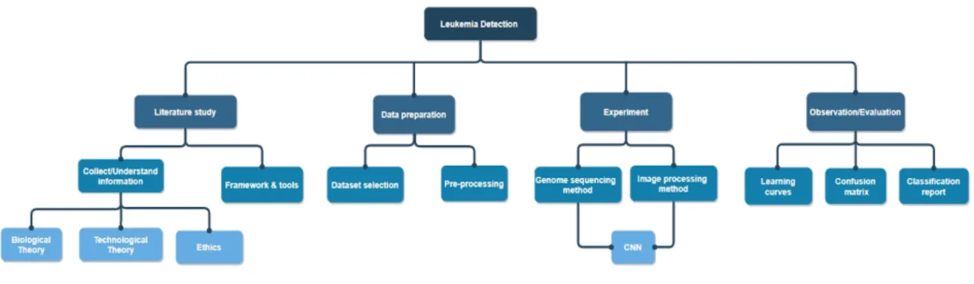
In the process of gathering information, ACM, IEEE, and Google scholar was used to find articles and journals that discuss subject relevant to the project which is presented in related work in chapter 3 and further analyzed in chapter 6. The planning of the project is presented in the problem tree. The tree is an overview of the essential aspects of this comparative study. Figure 5 shows the four-section, empirical study, data preparation, experiment, and evaluation. The tree branches are further described in detail in section 5.1.

Figure 5. The Problem tree

5. 1.1 Literature study

The collecting and understanding branch is in the theory chapter, section 2.1-2.4, and it is done to provide a better understanding of the subject of machine learning and the influence it has on biomedicine. When examining various framework and tools, such as Jupyter notebook and various libraries were examined, such as sklearn, numpy, panda and keras. These libraries were used to construct and implement the methods.

In this process,_{​Google Collaboratory​}(Google colab) was used, which is a free cloud-based replica of the Jupyter notebook software. Google colab comes with an extensive library and has the most common deep learning applications. It can process algorithms, and this can be accessed through a Google account which connects to Github to download or upload repositories. The software codes are written in the program language Python and can create and illustrates graphs and matrices [1].

Tensorflow is an open-source software library that uses mathematical algorithms that can handle tensor operations. The library expresses output in graphs and n-dimensional matrix. It has modularity attributes, which makes it flexible and is easy to use for training architecture. Tensorflow can process and train multiple networks. Therefore, it is useful when working with a larger system [2].

Keras is a neural network library in Python that uses Tensorflow in the backend infrastructure to compile models and graphs for machine learning. It can be implemented in almost every neural network models and be processed on both CPU and GPU with high speed. Keras is commonly used and is easy to implement when working with images or text [3].

Scikit-learn is a Python library that can be used when implementing algorithm(s) in difficult model training. It contains numerous functions, such as classification and model selection. The library has features like cross-validation that calculates the accuracy of the model. Scikit Learn also handles unsupervised neural networks and feature extraction to retrieve information from images or text [4].

Numpy is a machine learning library that works along with other libraries to perform array operations. The library is easy to use for complex mathematical implementations. These features are applied when working with expressing binary in an array of n-dimensions, images, or sound-waves [5].

Panda is a library in Python that has multiple different features for analysis of data structure. The library has built-in functionalities such as translation of operation and data manipulation, which provides flexibility with high functionality [6].

5. 1.2 Data preparation

For data preparation, the collection and preprocessing of the dataset is an important step. This describes where the datasets are collected from and sites that have databases with images from blood samples. The preprocessing stage is when datasets for both methods are gathered and prepared by formatting the size on the genomic sequences and images. That it is to adjust them to the models, this step describes where the dataset is from and pre-processing preparation steps.

5.1.3 Experiment

The experiment stage consists of two models: the cancer marker detection method and the blood smear image for the leukemia detection method. The models are trained one at a time and implement CNN architecture. This stage describes every step that occurs during the experiment phase. It explains how the datasets are uploaded and pre-processed. The models' datasets are using 3-way cross-validation to divide them. The datasets are classified into a training and testing set with a 75:25 split. 75% are for training, and 25% are for testing. The training set is further divided with a ratio of 75/25, where 75 % are for training the model network, and the remaining 25 % is for validation. This section also describes how the models are trained and tested but also how they implement classification functions.

5.1.4 Observation & Evaluation

In this step, both methods have produced results which are analyzed individually and compared with each other in section 5.4 and chapter 6. It is to discuss the challenges and benefits of both models and how they performed under certain circumstances. The model uses a learning curve during the training process to estimate their performance and confusion matrix as their classification report. The produced results in section 5.4 are going to measure the prediction quality and accuracy of the models.

5.2 System design

In this section, the architecture system was developed and described the data preparation process in figure 6. It was an important step and showed the selection of the dataset and preparations for them.

Figure 6. Design of the system

5.2.1 Collecting datasets

This step describes the finding and making of a dataset for both methods. It explains the necessary pre-processing preparation of the data samples that will occur before implementing into the models.

5.2.1.1 Genome dataset

National Center for Biotechnology(NCBI) is a national institution of health, that has a database containing resources for biotechnology and informatics tools. NCBI holds a major Gene bank that stores billions of nucleotide base pairs [7]. The data sample used for the genomic sequence method was from NCBI Genebank. On their website, there is a customizing search function. It helped to narrow down the search result from their large database. In the search field, leukemia was entered, and the settings were changed to homo-sapiens, and the amount of nucleotide to least be 100000 bp. This would have eliminated any search results of other species. The cancer dataset has cancer annotation, which is the cancer markers, and this has been handled by professional biotechnical. The samples used were in Fasta format and had a sample size of 10500 bp and placed in a text format with 2000 row each containing 50bp. Each row in the dataset was considered as one input.

→

a) _{​An example on a part of raw dataset ​b) dataset cleaned and integrated} Figure 7. Genome dataset being formatted

Once all the data was gathered, it needed to go through pre-processing, which meant formatting and reshaping the dataset. Figure 7a shows the raw data with space, annotation numbers, and not shaped into a matrix with dimension 2000 by 50. The formatting was performed manually by transferring all sequences to a plain text document. All numbers from each row were then removed. Afterward, the number of nucleotides in each section was counted to ensure that there were 50 nucleotides on each row. The space between any letters was removed. Once the dataset looks like figure 7b, it was ready for the pre-processing step in figure 8.

5.2.1.2 Blood smear images

The blood smear data samples were pictures of white blood cell subtypes that were part of the BCCD dataset. These samples are also in BCCDs GitHub or Kaggle profiles. The data sample contains 10000 images in JPEG format that have been verified by experts. The WBCs were color dyed to be more visible for the algorithm to recognize the abnormal cells. It also has cell-type labels in a CSV file, and in each folder, there were around 2500 augmented images of each cell-type.

a) _{​Lymphocytes ​}b) Eosinophils

c) Monocytes _{​d) Neutrophils}

Figure 9. microscope images of different white blood cells

The images dimension were downsampled from the 640x480 to 120x160 so that the model could be trained faster. The datasets were split into training and testing sets, and there were images for every type of WBC. The images were augmented to increase the sample size and variation so that there was an equal amount of images of the different cell types in each training and testing folder.

5.2.2 Pre-processing

The pre-processing data prepared the relevant datasets for implementation. The step consisted of four sections, which are shown in figure 9. Cleaning data was done by identifying and removing inconsistent attributes that were wrong. This was to reduce the possibility of having a result that could be inaccurate or not accepted by the model. Removing spaces and characters is considered a form of cleaning the dataset. The integrating process compiled the datasets to avoid redundancy and confusion about the same variables referring to different values. After cleaning and integrating the dataset, it needed to be transformed into an appropriate form that the models' algorithm could execute. These forms were either an array or a matrix.

Figure 9. Pre-processing phases

The data compression process was to make the data ready by using label encoding and one-hot encoded and converting the bases into a numerical matrix form with 4-dimensional vectors. The nucleotide was assigned with a number from 0 to 3. This created a numerical order which gave the dataset a context that the algorithm could easily understand.

Now that the nucleotides have label-encoded values, it created a number order that might confuse the model. What made the model confusing was that it believes the input values' implementation order creates a hierarchy so that adenine was always first despite the input sequence. By using the one-hot encoding method from scikit- learn the hierarchy problem would be resolved. This transformed the sequences by creating four columns and converting the values into a four-digit binary code which can be seen in table 2. The previous numbers were replaced with zeros and ones and placed each digit in a column. Each row corresponds to one of the nucleotides that have a predefined value that was written in the cells.

5.3 Model implementation

5.3.1 Genomic Sequencing - Method 1

The datasets were uploaded through a URL that held the raw dataset in a text file. The _​filter() function ensured removing all empty sequences and organizing the data into a format that could be processed. The DNA sequence was transformed into a matrix. It was done with one hot encoding from Sklearn._{​LabelEncoder() converted the bases into an array of integer, and the ​OneHotEncoder()} turned the integer array into a matrix.

The dataset was split into training and testing with the _{​train_test_split() from} sklearn.model_selection function. The training set was further divided into validation and training set with_{​validation_split} = 0.25_​, which stored parts of the dataset to see if the dependent values are cancer or not a prediction. The network architecture for this model was a 1D convolutional neural network. The model used library Keras to construct the network easily and applied conv1d with the filter=32 and kernel_size=12. The 32 filters were down-sampled in the pooling layer that uses MaxPooling1D. The matrix from the different pooling layer was prepared by transforming into columns into CNN's next layer. The activation function in the dense function was _{​activation='relu'} applied on the layer with 16 tensors, and the second activation function used was softmax.

After training the method, it used the binary classification task to plot the accuracy and loss of the network and presented a learning curve. Before using the compile function, the model measured its loss using binary_crossentropy_​. The metric used for accuracy was _{​binary _accurac​}y label, which presented the amount of prediction that matched with the dependent variables. For the evaluation, the model uses a confusion matrix with the _{​confusion_matrix() ​}from Sklearn.

5.3.2 Image processing- Method 2

The pre-processing of the images consisted of both augmenting the images and applying a color enhancer to make the WBC cell appear more on the RGB scale. This was so that the images could be more recognized. It was done by using _{​cv.imread()​}. With the TensorFlow_{​model.Fit() module from} Keras TensorFlow, an array was created by placing them in a variable that converted them into an integer. The CSV file with labels was one-hot encoded. The data samples were split into training and testing with the _{​train_test_split()​}. The training samples were divided into _{​validation_split=0.25​}. It meant that 25 percent of the training data was used for validation. To ensure that the values were randomly sampled, a random module was used to shuffle the images so that there were different images with every new test. This model used 2D convolutional kernels to train the model, and as previously mentioned in chapter theory, consists of multiple layers that the images process through. To detect possible negative values in a matrix of the image dimension, CNN extracted the input layer and used activation function ReLU, _{​activation='relu'​}. The images were too large to be processed, so the model applied a pooling layer by calling Keras Max Pooling to reduce the size to 120x60. The dropout layer had Dropout =0.1 on the first layer, 0.2 on the second, and 0.40 on the last. These numbers are percentage values and indicate the amount of the neurons randomly assigns with zero weights. The fully connected layer applies_{​activation=' softmax' to produce output from}

all the features layer in the model.

Learning curves were used to measure the performance of the trained model. With a multi-class classification problem, the optimizer was _​'adam'​, and the loss function was is set on

loss='categorical_crossentropy',_​and the accuracy metric was_{​'accuracy.' After training the model, it} used a plot function to plot the result. The model also created a confusion matrix.

5.4 Evaluation

This section presents the result from the genomic sequencing method in subchapter 5.4.1 and the image processing method in subchapter 5.4.2.

5.4.1 Genomic Sequencing result

This method's purpose was to detect cancer markers on DNA sequences from cancer cells. In this test, a dataset with 2000 rows of DNA sequences was used. Each row contained 50 nucleotides. The epochs were set on 50 to train the model. The two figures below 10a-b show the performance of the model. The accuracy measured the model prediction performance, and the model loss presents the uncertainty of the model prediction. The distance between the training and validation line is small in figure a, and in the accuracy plot. The training and validation line starts to divert from each other at around 0.92 and stops approximately 0.97.

a) A plot of the models loss b) A plot of the model final accuracy

c) Confusion Matrix result

The confusion matrix shows that the model had a prediction score of 0.97, TP, which means that it found markers and correctly identified them with a 97% rate. The TN had a 99 % rate of correctly predicting non-cancer marker. The two error type class had a low percentage with 3% and 1%.

5.4.2 Image process result

The model used accuracy and validation loss to decide the trained model's performance and was presented below in figure 11a-b. It also used the confusion matrix to display the accurate detection of the different subtypes of white blood cells. The method's purpose was to locate the four types of white blood cells, eosinophils, lymphocytes, monocytes, and neutrophils. To determine the diagnosis was cancer or not depends on if the level of WBC were high or low from CBC.

a) plot for model loss during training b) plot for accuracy of the model’s performance

c) Confusion Matrix of result

The model loss and model accuracy in figure 11a-b showed that the distance between the validation and training line was small, but around 40 epochs, the line distance starts to divert from each other. This could indicate that the model had a relatively high prediction value, which in figure 11c shows the accuracy is 80.5%, which was produced from accuracy_score using prediction values from sklearn metrics. The confusion matrix also had the numbers from 0-3. These numbers represent the four WBC types in the order; neutrophil(0), lymphocytes(1), monocytes(2), and eosinophils(3). It shows that the eosinophils(3) have had a higher correct prediction compared to the other WBC types and the lowest false predictions. In Section 2.12, the table presented the ratio between different WBC types for normal blood levels. The number of monocytes and eosinophils should be less than neutrophils and lymphocytes. It increased the levels in WBC 2 and 3 but also decreased WBC type 0, and 1 was an indication of leukemia.

5.4.3 Classification Report

This section presents the classification report on both methods. It measured the quality of the methods' prediction based on the confusion matrix from section 5.4.1-2. The calculations were based on the equation 2-6 in section 2.2.5 and compiled into two tables. The tables below display the prediction accuracy for each class and the total accuracy. It is the overall performance of the entire method.

Table 3 shows the classification report for the first method for genomic sequencing. The reported accuracy was similar to the accuracy in the confusion matrix plot in section 5.4.1. Class 0 is positive cancer markers, and class 1 is for non-cancer markers.

Table 3. Classification report of genomic sequencing method

Class Recall Precision F1-score Total Accuracy

0 0.97 0.99 0.98

0.98

1 0.99 0.97 0.98

The classification report for image processing was compiled and presented in table 4 and displayed the recall, F1-score, precision, and accuracy for each white blood cell. It also shows the entire method of total accuracy.

Table 4. Classification report of image processing method

Class Recall Precision F1-score Accuracy

Neutrophil (0) 0.61 0.88 0.72

0.81

Lymphocytes(1) 0.83 0.69 0.75

Monocytes (2) 0.93 0.75 0.83

6 Discussion

6.1 Method analyzation

The methodology used in the project is Takeda's GDC method, which was described in section 4.1 because of its iterative ability and flexible structure on each step. Those were essential qualities because each method was tested repetitively with different hyper-parameters to find the optimal choices that produced a result with the highest accuracy possible. The final results were achieved after testing the methods and presented in section 5.4. The structure of the thesis, which was a comparative study that did not necessarily require a complex methodology structure such a Nunamaker, which was better suited for engineering work with more advanced projects with multiple different work areas [46]. The Takeda method was simple and had a flexible formation. This meant that the steps could be redefined to fit one's interpretation of the model as long as it followed the general principle of the methodology. Chapter 5's structure was based on each step of the GDC method and presented what each phase produced.

6.2 Reflection on related work

The related works section were papers on studies that were similar or had some relevance to this project. Each article was relevant to a particular aspect of the project, such as genomic sequencing or deep learning in general. In the article _{​3.4 Predicting the sequence specificities of DNA- and} RNA-binding proteins by deep learning, the author discussed a deep learning model that process DNA sequences in proteins to search for diseases and to detect them [10]. The model applied a Convolutional neural network and split the data in 3-way cross-validation. The dataset contained 100000 bp, which is around 2000 row in a fasta format and had accuracy on 93%. The total accuracy for methods 1 and 2 was in section 5.4.3, which were 98% and 81 %, respectively. An explanation for how the first model scored a higher accuracy could be that the dataset used was smaller compared to the images dataset, which has 10000 images. The datasets sizes were adapted to suit each method the best; reducing the image process dataset would be ineffective in reducing bias in the method and making the model overfitted. Finding an equally large dataset for a genomic sequence is a difficult task, and manually pre-processing the dataset would be time-consuming. The genome model is also a binary classification, and the only purpose was to classify markers that are either cancer or not cancer. This narrowed down the model's work, but also that the model was a simple CNN implementation compared to the model in section 3.4, which was a multi-classification.

In the paper called_{​Artificial intelligence in digital pathology: a roadmap to routine use in clinical} practice_​, the author wrote about integrating image software tools and transitioning from manual work to an automated process [8]. This paper directed its attention to histopathology, which was similar to the second method that processed images of blood smear. The WBC test had mostly been done manually, and only in recent years, the work process had been more automated. Automation of pathology test speeds up the process and reduce waiting time which the article mention.

In article _{​Artificial intelligence in healthcare: a critical analysis of the legal and ethical} implications_​, the author discussed the beneficial aspect of AI in healthcare but also ethical issues [11]. The author brought up problems such as discrimination and data intrusion that can occur when handling sensitive information that belongs to the patients. This thesis used DNA sequences that are collected from humans. Despite not having a major problem finding a sample, the NCBI website did not disclose the number of people that the sample belonged to and only had a limited dataset for public use. The blood sample images were more challenging to find because they needed to come from patients with leukemia, and most sites required a filled in consent form need to be sent to the owner of the samples to use them. These were the protocols and guidelines that could be based on the GDPR law mentioned in section 2.6. The law makes it difficult the work with machine learning because it protects the information owner's privacy.

6.3 Analysis result

The thesis was a comparative study and used a different method whose purposes were to detect cancer in their respective data samples. Both methods had a Convolutional neural network architecture. The models were evaluated in section 5.4 with a classification report, learning curve, and confusion matrix. These different evaluation tools were implemented to analyze each model's performance and compared them with each other. The RQ 2.2, which is _{​What differentiates the}

accuracy of these two tests for the outcome result? It could found in section 5.1, which presented the first method that processed the nucleotide base. The section showed that the model was well trained, where the validation and training line showed a small distance. The lines start to flatten out around 0.97, which were around the same level where the model reached its highest accuracy—comparing the result with the confusion matrix True positive, which were also 0.97 indicated that the plot was accurate.The interpretation of the values was that the model labeled 97 % of the cancer markers correctly. The total accuracy for the entire method was presented in the classification report in section 5.4.3 and had an accuracy rate of 98%.

The second method processed blood-smear images and performed a WBC test. It detected and counted the number of white blood cell types to compare each WBC level to the reference table in section 2.1.2 and decided whether a patient had cancer. Section 5.4.2 presented the model loss and model accuracy from training the method. It showed that this method was not as well trained as the previous method. The accuracy of the method was not presented in the confusion matrix in percentage, as previously done in section 5.4.2. This was because the WBC test needed to count the number of white blood cells that had been detected.

After all, the level of each cell determined the cancer results—average blood level neutrophil and lymphocytes should have the highest number. Still, the results showed there were low levels of neutrophil and lymphocytes high levels of monocytes and eosinophils. The abnormal levels with the WBC types indicated possible leukemia. The classification report presented the total accuracy of the model, 81 %, which was lower than the genomic sequence method. It clearly showed that the first model had a higher accuracy, and a factor for this could be because of the dataset. Despite having data samples from patients with leukemia, the accuracy difference can be due to genome samples were 2000 rows of sequence, and each line could be considered an input. The image sample had a size of 10000 images, which was five times the amount of genome models sample. The test required a larger dataset because reducing the number of the image would not produce an accurate representation of blood sample. It would only be a small portion of the whole sample and be an incomplete blood test. The classification report for the image processing method showed that the type errors for WBC types were already high and reducing the size of the images would further increase the type-errors. Reducing the sample for the WBC test would, therefore not be a good option because it could affect the accuracy of the test and it requires a certain amount of samples. Increasing the genome dataset would be difficult because finding a dataset large enough was hard to find, and it was even more challenging to pre-process manually. It could be a suggestion for future improvement to optimize the pre-processing phase and to make it completely automated. The number of markers was not a deciding factor for the genome method's diagnoses, and this was the significant difference between these two tests. Also, the WBC test was a multi-class classification and handled more parameters compared to the genomic method, which only worked with two labels: cancer and non-cancer marks. This made the second model slightly more complex and required more testing.