Distributional effects of taxes on car fuel, use, ownership
and purchases
Jonas Eliasson1, Roger Pyddoke2, Jan-Erik Swärdh2
1Department for Transport Science, KTH Royal Institute of Technology
2Division of Transport Economics, VTI Swedish Road and Transport Research Institute
CTS Working Paper 2016:11
Abstract
We analyse distributional effects of four car-related tax instruments: an increase of the fuel tax, a new kilometre tax, an increased CO2-differentiated vehicle
ownership tax, and a CO2-differentiated purchase tax on new cars. Distributional
effects are analysed with respect to income, lifecycle category and several spatial dimensions. All the analysed taxes are progressive over most of the income distribution, but just barely regressive if the absolutely highest and lowest incomes are included. However, the variation within income groups is substantial; the fraction of the population who suffer substantial welfare losses relative to income is much higher in lower income groups. The two most important geographical distinctions are between rural and urban areas (including even small towns), and between central cities and satellites/suburbs; these spatial dimensions matter much more for distributional effects than for example whether an area is remote or sparsely populated.
Keywords: Distributional effects, equity effects, fuel tax, car ownership tax. JEL Codes: D63, H23, R48.
Centre for Transport Studies SE-100 44 Stockholm
Sweden
3
1
INTRODUCTION
Taxes on vehicles and motor fuel serve important roles both as sources of tax revenue and as policy instruments. First, fuel and vehicle taxes are often attractive fiscal instruments due to the comparatively low price elasticity of both car use and ownership. Second, the externalities of motorized traffic motivate pigouvian taxes on car use, such as carbon taxes and congestion charges. While taxes on car ownership and purchases are usually purely fiscal instruments, they are also increasingly motivated with climate policy arguments, for example subsidies for alternative-fuel cars.
In practice, an important constraint on the design of all these tax instruments is their distributional effects. There are widespread concerns that such tax instruments may have unwanted distributional effects, such as being regressive or hurting rural areas more than urban areas. The purpose of this paper is to analyse such distributional effects.
We analyse four tax instruments: an increased fuel tax, a kilometre tax, an increased CO2-differentiated vehicle tax, and a new CO2-differentiated purchase tax on new cars.
Their distributional effects are analysed with respect to income, lifecycle category and several geographic dimensions, e.g. urban vs. rural areas, large vs. small cities and central cities vs. suburbs/satellites. Presenting all possible combinations of tax instruments and distributive dimensions would create a bewildering number of results. Therefore, we aggregate various geographic dimensions as the analysis proceeds, revealing which geographic dimensions are the most relevant.
Our analyses are based on data from Swedish administrative registers, comprising data on all Swedish adults and cars. Sweden is an interesting case study from an international perspective for several reasons. First, the geographical variation is very large: residential areas vary from dense urban areas with high public transport shares to very sparsely populated areas sprinkled with small towns and villages with long distances in between. This means that although the average distance by car per person is similar to most developed European countries, the geographic variation in living circumstances is very high. Second, Sweden has among the smallest income inequalities in the world, but there is enough income variation to let us explore whether the analysed tax instruments are regressive. This is interesting because it sheds light on equity effects of car-related taxes in a society where a large majority of households can easily afford to own and use cars. Even if this is still an exception in a global perspective, more and more countries are approaching this situation. Third, access to complete register data means that we can conduct detailed analyses even of small cross-segmentations. This means that we do not have to use modelling approaches to extrapolate from a limited sample of observation, as many other studies have needed. In any distributional analysis, changes can either be presented as absolute numbers (e.g. euros per person) or relative to income. We will usually report both results, but since conclusions may depend on which of these measures is considered, the question remains which one is the most relevant. In our view, this depends on what the purpose of the tax is. If the purpose of a tax increase is simply to generate public tax revenues, then it is natural to compare its distributional profile to a flat-rate income tax. This is the classic definition of regressivity: a tax is regressive if the poor pay more than the rich relative to their income.
However, if the purpose of the tax is to correct prices for external effects, then it is less clear that measuring changes relative to income is relevant. After all, prices are almost always the same for everyone, regardless of income or wealth. The desire for increased
4
income equity is instead usually handled by taxation and welfare systems (with the addition of a few special policy measures such as subsidized healthcare and housing). If the default position therefore is that prices are, generally, equal for everyone – with a few, deliberated exceptions – it is natural to argue that the distributional effects of corrective taxes – taxes which are introduced to make the prices “right” in the sense that they reflect full social costs – are in fact essentially irrelevant. At least, one should realize that arguing against corrective taxes with distributional arguments is logically equivalent to arguing that the good in question (car travel, for example) should be subsidized for distributional reasons – and this is often a much less persuasive or intuitively appealing argument.
However, there are two relevant arguments to consider distributional effects also when introducing corrective taxes. First, any change causes transition costs which may be important to consider, at least for determining at which speed a change can be implemented. Second, many countries have regional policies intending to support rural, remote or sparsely populated areas. It is often argued that taxes on car use harm such areas disproportionately. If this is true, then it may be wise to abstain from full internalization of the external effects of car traffic. The argument is essentially that subsidizing car use, by not aiming at full internalization of social costs, may be an effective policy for supporting rural or remote areas. To what extent this argument holds water is one of the questions of the paper.
Hence, being aware of the distributional effects of taxes on car use and ownership is clearly worthwhile for applied policy making. Moreover, most public debates on such taxes allude to various distributional effects – positive or negative – so exploring their real sign and size is also important for facilitating a more informed and realistic public debate.
There is an extensive literature on the equity effects of gasoline taxes. A recent book (Sterner, 2012a) reports results from over two dozen countries, concluding that while there may be some slight regressivity in some high-income countries, fuel taxation is generally a progressive policy, particularly in low income countries; gasoline taxes tend to become more progressive the lower the average income of a country is. The main results are summarized in Sterner (2012b). Bureau (2011) uses French household data, and concludes that a fuel tax is regressive. Santos and Catchesides (2005) study UK data, finding that middle-income households suffer the most. When they limit the sample only to car-owning households, they find that a fuel tax is regressive. This is a similar conclusion to Blow and Crawford (1997) (cited in Bureau (2011)), who find that fuel taxes are progressive if all households are considered, but regressive if only car-owning households are considered. Bento et al. (2009) analyse US data, concluding that under flat revenue recycling, a fuel tax increase is progressive, while income-based recycling has a U-shaped impact pattern. That net equity effects depend on how revenues are recycled is also stressed by e.g. Bureau (2011) and Eliasson and Mattsson (2006) (analysing congestion charges).
There are much fewer studies of distributional effects in geographic dimensions. Bureau (2011) distinguishes between urban and peri-urban/rural residents, showing that welfare losses are substantially lower in urban areas.
5
2
DATA AND METHODOLOGY
2.1 Data sources
Data come from Statistics Sweden and the Swedish vehicle registry, and contains all adults and all personal cars in Sweden. There are advantages with using register data, but also limitations. Behaviour is only observed from what can be found in registers. This means that we do not know for sure where individuals actually live, which car they drive and how much. What we know is where people are registered to live, which cars they are the registered owners of, and how many kilometres these cars are driven. Moreover, we do not have access to household data, only individual data.
The vehicle data set contains all private cars owned by individuals in Sweden in the year 2011: 4.84 million cars distributed over 3.51 million car owners. For each car, we have data on vehicle kilometres driven per year1, registered fuel consumption and
registered CO2 emissions per kilometre, the owner of the car, and a number of other vehicle characteristics such as weight and length. The population data set contains all 7.56 million adults in Sweden in 2011 (the total Swedish population is 9.48 million). Each record contains data on disposable income, gender, age, employment status, residential location and workplace location. “Disposable income” includes all types of income after tax, including welfare transfers, pensions and unemployment benefits and so on.
Some records are excluded from the data set: deregistered cars, rental cars, commercial vehicles, cars with a weight over 3 500 kg, and individuals who own more than four cars (since there is an apparent risk that these cars are not exclusively used by the owner and the owner’s family)2. We also exclude individuals with income less than
30 000 SEK/year (10 SEK 1€) when calculating welfare effects relative to income. The reason is mainly that such very small incomes will lead to extremely large welfare effects when the income is in the denominator, which will distort the results. Even after this exclusion, one should be careful when interpreting the results for the lowest income group. Realistically, many of those who have very low registered incomes are likely to receive income from other sources, such as parents or spouses, since the registered incomes are well below the threshold for receiving various welfare benefits. Around 386 000 cars and 48 000 individuals are excluded for the reasons above.
Imputing and adjusting fuel consumption and carbon emissions
The vehicle registry only contains data on fuel consumption for cars with vehicle year 2005 and newer. Since fuel consumption is essential for our calculations, we have to impute it. We do this using an OLS model estimated on vehicles from the years 2005-2009, regressing fuel consumption on vehicle characteristics (weight, length, width, petrol or diesel, type of car body) and a linear time trend to account for the fact that newer cars are more fuel efficient. The model has a sufficiently good explanatory power for our purposes (R2=0.61).
For most cars, we have data both for registered fuel consumption and registered C02
emissions, but for some cars, data on CO2 is missing. For these cars, CO2 emissions are
1 More precisely, the vehicle kilometers between two vehicle inspections.
2 This limit is of course somewhat arbitrarily set. On the other hand, we have to set some exclusion
6
calculated based on fuel consumption, assuming 2.14 kg CO2/litre petrol and 2.26 kg
CO2/litre diesel. 3
The data in the vehicle registry only contains registered fuel consumption. However, there is substantial evidence that actual fuel consumption exceeds registered fuel consumption, and that the difference is increasing over time (Mock et al., 2013). Therefore, we adjust the registered fuel consumption figures with the estimated differences between actual and registered fuel consumption (and CO2 emissions) in
Mock et al. (2013), using the average of one study from Spritmonitor.de (Germany) and one study from Honestjohn.co.uk (United Kingdom). The adjustments factors can be found in the Appendix (Table 10).
Imputing kilometres driven for company cars
Company cars (or “benefit cars”) are cars owned by a company and used by an individual, partly on duty and partly for private purposes. From our data, we know which individuals who have access to a company car, but there is no data about the car – neither distance driven, nor fuel consumption, nor CO2 emissions. For company cars,
we impute distance driven based on an OLS model estimated on all cars owned by employed individuals, where distance driven is regressed on the owner’s disposable income, age, number of children, distance to work, number of owned cars, gender and geographical region. The model has low explanatory power (R2=0.07), but the
calculated average distance of company cars still exceed the average of privately owned cars (17 420 km/year compared to 14 832 km/year). There is still a risk that the distances driven for company cars are underestimated, but there is no other solution, and leaving company cars out of our analyses would clearly distort the results.
We assume that company cars are driven on petrol and have a fuel consumption of 0.06 litre/km. The tax regulation stipulates that an individual with car and fuel benefit (i.e. fuel is paid by the employer) pays a fuel benefit tax corresponding to 1.2 times the fuel cost. There are also individuals with car benefit only, who pay the fuel out their own pocket. We assume that all individuals pay the fuel benefit tax and have a marginal income tax rate of 52 percent, which means that they pay the equivalent of 62 percent of normal fuel costs.
2.2 Calculating the welfare loss of a tax increase
We use the change in consumer surplus as a measure of the welfare loss of a tax increase (before recycling of tax revenues). The change in consumer surplus consists of two parts: a monetary cost equal to the increased cost for those individuals who do not change how many cars they own or how much they drive, and a welfare loss for those individuals who decrease the number of cars they own or how much they drive. To calculate the second part we need elasticities of car use and car ownership with respect to cost. We use elasticities adapted from Pyddoke and Swärdh (2015), which are differentiated according to income, gender and type of residential location (urban, rural near an urban area, and sparsely populated). The elasticities can be found in the Appendix (Table 11). This second part of the consumer surplus (the welfare loss of changing car use or ownership) is substantially smaller than the first part (the direct monetary cost): typically, it only consists of 1-2 % of the total welfare loss4.
3 These figures are the median ratio between fuel consumption and CO
2 emissions in our data for
petrol cars and diesel cars, respectively.
4 It can be shown that the relative size of the second part of the consumer surplus, i.e. the “triangle
under the demand curve” relative to the “rectangle under the demand curve”, given a relative price change a and demand elasticity 𝜖 is 𝑎𝜖/2. The tax changes we study are in the order of 5-10%
7
2.3 Descriptive statistics
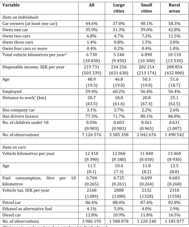
Table 1. Descriptive statistics. Standard deviations in parentheses.
*Distance to work are based on employed individuals only
Table 1 summarises descriptive statistics, split by type of residential area. These area types are defined as follows. An “urban area” is a contiguous area where distances between houses do not exceed 200 m, and the total number of inhabitants in the area exceeds 3 000. Note that the term “urban area” also includes quite a few small villages. Non-urban areas are defined as “rural”. “Large cities” are defined as urban areas in the
changes in the kilometer cost, and the demand elasticities are in the order of -0.3, giving a relative size of the second part of the consumer surplus of around 1%.
5 Note that a large share of individuals have zero cars and hence zero vehicle kilometers, which makes
the standard deviations large.
Variable All Large
cities Small cities Rural areas Data on individuals
Car owners (at least one car) 44.6% 37.0% 48.1% 58.3% Owns one car 35.9% 31.3% 39.0% 42.8% Owns two cars 6.8% 4.7% 7.2% 11.5% Owns three cars 1.4% 0.8% 1.5% 3.0% Owns four cars or more 0.4% 0.2% 0.4% 1.0% Total vehicle kilometres per year5 6 730
(10 830) 5 240 (9 450) 6 890 (10 300) 10 110 (13 530) Disposable income, SEK per year 219 731
(503 339) 234 256 (631 638) 202 214 (213 174) 208 854 (432 800) Age 48.9 (19.3) 46.8 (19.0) 50.3 (19.8) 51.6 (18.7) Employed 59.4% 60.2% 56.4% 56.4% Distance to work* (km) 20.7 (63.5) 18.8 (61.6) 20.8 (67.4) 25.1 (62.5) Has company car 3.1% 3.7% 2.2% 2.6% Has drivers licence 77.3% 71.7% 80.1% 86.8% No. of children under 18 0.596
(0.983) 0.603 (0.983) 0.561 (0.965) 0.631 (1.007) No. of observations 7 126 576 3 585 358 2 042 676 1 498 542 Data on cars
Vehicle kilometres per year 12 410 (8 390) 12 060 (8 180) 11 840 (8 030) 13 460 (8 930) Age 11.5 (8.1) 10.4 (7.3) 11.8 (8.2) 12.5 (8.8) Fuel consumption, litre per 10
kilometres 0.704 (0.265) 0.725 (0.261) 0.699 (0.264) 0.683 (0.268) Vehicle tax, SEK per year 2168
(1389) 2088 (1288) 2132 (1328) 2310 (1558) Petrol car 86.4% 88.4% 87.4% 82.8% Ethanol as alternative fuel 4.1% 5.0% 4.0% 2.9% Diesel car 12.8% 10.9% 11.8% 16.5% No. of observations 3 986 195 1 580 078 1 220 240 1 185 877
8
three major metropolitan regions (greater Stockholm, greater Gothenburg and greater Malmö) and in municipalities where the largest city has at least 60 000 inhabitants. “Small cities” are the remaining urban areas. 50% of Swedish adults live in large cities, 29% in small cities and the remaining 21% in rural areas.
Car ownership, license holding and car use is higher in rural areas and lower in large cities. Distance per car, however, is similar in all area types. Income is lower in rural areas and higher in large cities. Cars are older but have better fuel economy in rural areas, while they are newer but have worse fuel economy in large cities. The difference in fuel economy may partly be due to diesel cars being more common in rural areas: diesel cars become more economically preferable the more the owner drives, since the fuel cost per kilometre is lower but the vehicle tax is higher.
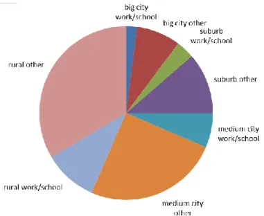
To give a better understanding of travel patterns, and in particular the sources of CO2
emissions, Figure 1 shows the share of total VKT (vehicle kilometres travelled) for private trips by trip purpose (“work/school” and “other”) and type of residential location: “big city” (municipalities with more than 200 000 inhabitants: Stockholm, Gothenburg and Malmö), “suburb” (suburb municipalities of the big cities), “medium city” (municipalities with 50-200 000 inhabitants) and “rural” (all other municipalities). This data come from the National Travel Survey, since this is the only way to get access to trip purposes; the vehicle registry data used in the rest of the present study allows a much more detailed analysis in terms of geography and income, since it includes all Swedish vehicles.
Figure 1. Car distances split by trip purpose and type of residential location. Data from the National Travel Survey 2006.
The diagram shows that “other” trips contribute a much larger share to total driving distances than work/school trips. The diagram also shows that from a climate policy perspective, policy measures focusing on metropolitan areas will be far from enough: around three quarters of emissions are generated in medium-sized or rural municipalities. Work trips in metropolitan areas, which often take centre stage in the public debate on transport policy, contribute around 5% to total CO2 emissions (adding
9
3
POLICY INSTRUMENTS AND OVERALL EFFECTS
We will analyse four policy instruments: a fuel tax, a kilometre tax, a vehicle ownership tax and a purchase tax for new cars (i.e. a vehicle registration tax). The latter two are differentiated with respect to the CO2 emission rate of the vehicle. In this section, we
describe the policy instruments and their calculated aggregate effects, and also describe the current Swedish situation to provide some background.
The policy instruments are designed to make them roughly comparable. The fuel and kilometre tax are set to make their calculated effects on aggregate CO2 emissions equal.
The CO2-differentiated ownership tax is set to make its revenues equal to the revenues
to those of the fuel tax. (In the short run, a differentiated ownership tax does not change aggregate emissions, since the vehicle stock is given.) The CO2-differentiated
purchase tax is set such that the annualised cost of the car will be roughly equal to the assumed fuel tax increase during the first five years, while the lifetime cost will be around half the total cost of the fuel tax we analyse (assuming the current average emission rate, average driven distance per year and a realistic depreciation rate). The reason for this design is that there is some evidence that car buyers only consider the fuel cost during roughly the first five years, so differentiating the purchase price might be a way to reduce emissions at a lower political cost while still achieving roughly the same emission reduction6.
3.1 Fuel tax
The fuel tax in Sweden consists of three parts (tax levels7 are from November 2015):
energy tax (2.99 SEK/litre for petrol and 1.68 SEK/litre for diesel), CO2 tax (2.38
SEK/litre for petrol and 2.94 SEK/litre for diesel) and value added tax (25 percent on the price including taxes). The CO2 part of the petrol tax takes into account that petrol
fuel in Sweden contains 5 percent ethanol.
In our fuel tax analysis, we assume a 50 percent increase of the CO2 tax. This translates
into a 1.19 SEK price increase for petrol and a 1.47 SEK price increase for diesel, plus the increases in VAT which follow. We assume that both petrol and diesel cost 13 SEK per litre before the tax increase. Ethanol cars are assumed to be driven on petrol, since the current relative prices of petrol and ethanol means that this is the cheapest option. The calculated deadweight loss implies a social cost of 0.26 SEK per kilogram CO2
reduction. Note that this deadweight loss is for the consumer side of the car-use market only
3.2 Kilometre tax
Sweden does not have a kilometre tax. Our analyses are based on introducing a kilometre tax of 0.147 SEK/km. This figure is chosen so that the total CO2 reduction
becomes the same as for the increased fuel tax (effects are calculated using the elasticities in Pyddoke and Swärdh (2015)).
The calculated deadweight loss implies a cost of 0.34 SEK per kilogram CO2 reduction,
i.e. higher than for the fuel tax, as expected.
6 Another interesting approach would have been to try to design tax instruments that would have
achieved the same long term emission reduction. However, there are currently no results as to what effects differentiated vehicle or purchase taxes would have on long-term emissions.
10
3.3 Vehicle ownership tax
The Swedish vehicle ownership tax is differentiated with respect to fuel type (petrol or diesel), weight and CO2 emissions per kilometre (only for vehicles with registration
year 2006 and later). The motivation for differentiating the tax with respect to fuel type is because diesel cars emit more particulates. The CO2 differentiation was introduced in
2014, motivated by an intention to reduce CO2 emissions from cars. The CO2-related
part of the vehicle tax consists of a fixed part of 360 SEK and a variable part of 22 SEK per gram CO2 emission in excess of 111 gram per kilometre. For diesel cars, the CO2
-related tax is multiplied with a factor 2.37. If the car can be driven on ethanol the variable factor (22 SEK) is reduced to 11 SEK.
Our analysis of an increased vehicle tax is based on a 46.3% increase of the current vehicle tax. This figure is chosen to make short-run tax revenues equal to the revenues from fuel tax increase described above.
It is obvious that an increased ownership tax has no immediate effect on CO2 emissions,
since it does not change the cost of using the car. It may have effects on emissions in the long run, however, if a CO2-differentiated ownership tax makes car buyers choose more
fuel efficient cars – although it is disputed whether such an effect would be noticeable8.
What is clear, however, is that an increase of a differentiated ownership tax will affect the market value of the cars in the current car fleet: cars with better fuel economy will become more valuable and vice versa. If the tax change is substantial, it hence constitutes a considerable redistribution of wealth between car owners, but without any effect on CO2 emissions (at least in the short run). In our analysis, we do not
assume any behavioural responses to the increased car ownership tax, so the welfare loss for car owners is simply the increased ownership cost.
3.4 Purchase tax for new cars (registration tax)
Sweden does not currently have any purchase tax on new cars (a so-called registration tax), in contrast to Denmark and Norway where purchase taxes on new cars are very high. A government commission recently suggested a new, revenue-neutral purchase tax, differentiated according to CO2 emissions per kilometre to stimulate car buyers to
choose cars with better fuel economy. The argument was that since most new cars are bought as company cars, car buyers do not have enough incentive to consider a car’s fuel economy relative to its price tag. There is considerable empirical evidence supporting this argument (Greene, 2010), although there are also important studies contradicting it (Busse, Knittel, & Zettelmeyer, 2013). Another argument for the policy is that the fuel tax should ideally be set higher for climate policy reasons, but distributional concerns prevent this, so a differentiated purchase tax can be a second-best solution.
In order to analyse the welfare consequences of a purchase tax, we need to convert it to an equivalent annual cost for car owners in our sample. We do this by assuming that the purchase tax is annualized across the car’s lifetime proportional to the depreciation of the value of the car, which is approximated as a 15 percent depreciation per year compared to the previous year. In our analysis, this is akin to a differentiated car ownership tax which is also differentiated according to the age of the car. Since
8 There is some evidence that differentiated vehicle taxes do affect the CO
2 intensity of the vehicle
fleet in the long run (Giblin & McNabola, 2009; Ryan, Ferreira, & Convery, 2009). Forecasting the specific effects of a policy, however, has turned out to be difficult, primarily because it depends on reactions on the supply side (supply and pricing of vehicle makes and models) which are difficult to model (Hugosson, Algers, Habibi, & Sundbergh, 2014).
11
income groups tend to have newer cars, this difference has distributional implications. The yearly equivalent cost at year t for the purchase tax 𝑡𝑎𝑥𝑡 is calculated as
𝑡𝑎𝑥𝑡 = (0.85𝑡− 0.85𝑡+1)𝑀
where 𝑀 = 250[𝐶𝑂2− 90]+, i.e. 250 SEK for each gram of CO
2 emissions per kilometre
above 90 g/km. The factor 0.85 comes from our assumption that the car loses 15% of its remaining value each year. The purchase tax is equivalent to a price of 1 SEK per kilogram of CO2 emissions above 90 grams per kilometre assuming that each car is
driven 250,000 kilometres during its lifetime. As described above, the registration tax is similar to the increased fuel tax for a common new (diesel) car in Sweden9.
Differentiated purchase taxes have been shown empirically to have substantial effects on vehicle purchases (D’Haultfœuille, Givord, & Boutin, 2014), but just as noted above for differentiated vehicle taxes, it has proven difficult to forecast the effects of specific policies. For example, D’Haultfœuille et al (2014) describe how the effects of the French bonus/malus system became much larger than expected, in fact so large that the overall environmental effect was negative, since total car sales increased substantially when low-emission vehicles were subsidized. Hugosson et al (2014) compare forecasts of car purchases with outcomes, showing that forecasts are sensitive to assumptions about future supply.
4
DISTRIBUTIONAL EFFECTS ACROSS INCOME GROUPS
This section analyses distributional effects across income groups. To start with, we concentrate on first-order effects, i.e. without considering revenue recycling.
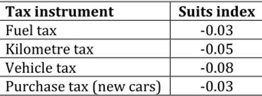
The first question is whether our four tax instruments are regressive, i.e. whether they hurt the poor more than the rich (remember that we measure the welfare change as the change in consumer surplus, not just monetary costs; the difference is small, however). We measure this with the Suits index (Suits, 1977), which measure the progressivity of a tax: a flat-rate tax has Suits index 0, a regressive tax has a negative Suits index and a progressive tax a positive index. The index is bounded between -1 and 1.
Table 2 shows that all the tax instruments are just barely regressive. The fuel tax and purchase tax are less regressive than the kilometre and vehicle taxes.
Table 2. Suits index (overall progressivity) of the tax instruments
Tax instrument Suits index
Fuel tax -0.03 Kilometre tax -0.05 Vehicle tax -0.08 Purchase tax (new cars) -0.03
9 If we assume a diesel car with declared fuel consumption of 0.06 litre/km the declared CO 2
emission is 136 g/km. This means that the actual fuel consumption is 0.076 litre/km. Assuming 20000 km driven per year during the first five years, the fuel tax increase implies 1.47*0.076*20000*5 = 11172 SEK in additional cost during these five years (without considering any discounting. Registration tax is (136-90)*250 = 11500 SEK, i.e. slightly higher than the fuel tax Note, however, that these figures are dependent on the assumptions about the life time of the car, the total driven distance, and the discount rate.
12
However, the story is more complex than is shown by the aggregate Suits indices. A closer analysis reveals that the negative Suits indices depend on the low and high tails of the income distribution. Table 3 shows relative welfare changes (welfare change as percentage of income) split by 8 equal-sized income groups (the table also shows the change in absolute terms). Except for the lowest and highest income octile, all tax instruments are in fact clearly progressive (relative welfare losses increase with income). The relative welfare loss is 30-80% higher for octile 7 than for octile 2, so the progressivity in these income segments is considerable. Octiles 1 and 8, however, break the pattern, since these groups contain individuals with very low and very high incomes, respectively. Relative welfare changes in octile 1 should be interpreted with caution: there are good reasons to suspect that the lowest incomes do not reflect individuals’ real access to money, since these incomes are well below the threshold for social welfare. The highest incomes in octile 8 are really very high – so high that car ownership and use cannot reasonably increase in proportion to income. The regressivity/progressivity of the taxes is hence different across the income distribution: between octile 2 and 7 they are progressive, but in the low and high tails they are regressive, since car use and ownership decline less than proportionally with income in the lowest octile, and increase less than proportionally with income in the highest octile. The overall regressivitity depends almost only on the highest octile.
Table 3. Welfare changes of the tax instruments, split by income octile. Absolute numbers and as percentage of income. Without revenue recycling.
Welfare change (consumer surplus),
SEK per year Welfare change (consumer surplus), as percentage of income (%) Income
octile
Average Income,
1000-SEK Fuel tax Kilometre tax Vehicle tax Register tax Fuel tax Kilometre tax Vehicle tax Register tax 1 61 -187 -256 -160 -138 -0.34 -0.47 -0.30 -0.25 2 107 -249 -357 -234 -201 -0.24 -0.34 -0.22 -0.19 3 138 -359 -513 -330 -307 -0.26 -0.37 -0.24 -0.22 4 171 -575 -792 -470 -475 -0.34 -0.46 -0.28 -0.28 5 210 -772 -1049 -569 -593 -0.37 -0.50 -0.27 -0.28 6 249 -1044 -1384 -730 -789 -0.42 -0.56 -0.29 -0.32 7 301 - 1332 -1708 -883 -1013 -0.44 -0.57 -0.29 -0.34 8 544 -1471 -1841 -957 -1219 -0.33 -0.42 -0.21 -0.27 Hence, we can conclude that all tax instruments are in fact progressive over most of the
income distribution – on average. However, this “on average” hides the fact that the variation within each income group is substantial. An income tax will by definition affect everyone with the same income in the same way. Our tax instruments are different: even if they are progressive “on average”, there may still be (perhaps many) individuals who are hurt disproportionately relative to their income. This is in fact the most important argument of those arguing against car taxes using distributional arguments: not that such taxes are necessarily on average regressive, but that there may be non-negligible subgroups who are hurt disproportionately.
We first explore this by splitting income octiles by residential location: large cities (urban areas10 where the central city has more than 60 000 inhabitants), small cities
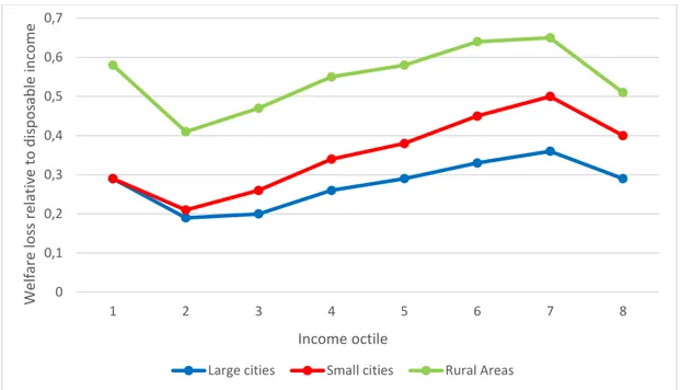
(other urban areas) and rural areas. Figure 2 shows the relative welfare loss (as percentage of income) from the fuel tax, split by income octile and type of residential location.
10 An urban area is defined as a contiguous area where distances between houses do not exceed 200 m,
13
Figure 2. Welfare loss of the fuel tax increase, relative to income, by type of residential location.
Clearly, there are substantial differences between types of residential locations. Indeed, the difference between types of location is often larger than the difference between income groups in the same type of location. For example, income octile 2 in rural areas would suffer a welfare loss of 0.4% of their income, which is more than the welfare loss of octile 7 in the large cities (as explained above, octiles 1 and 8 should be treated with caution). Conditional on location type, however, the fuel tax is still strongly progressive for octiles 2-7.
The differences in averages across income groups is explained mainly by differences in car ownership, rather than differences in driving distances across car owners (see Appendix, Table 13 and Table 14). In other words, if the analysis would include car owners only, all the tax instruments would be regressive, since the differences in driving distances are relatively small across car owners from different income groups. An even closer look at the variation within groups is provided by Figure 3. This diagram shows the share of each group (octile and location type) who suffers a welfare loss larger than 2% of their income, which is quite a lot worse than the average relative welfare loss, which is around 0.3%. The fraction in each group who suffer such considerable welfare losses are quite small – at most 6% (if we disregard octile 1). But the point is that this share is much higher in low income groups, and very much higher for low income groups in rural areas. Even if these groups are very small, there are up to four times as many in octile 2 as in octile 7 who can reasonably argue that they “are disproportionately hurt”, even when only comparing the same location type (the difference is much bigger between location types). For the purchase tax, the difference is even larger (full results can be found in the Appendix, Table 16).
This is probably what explains the commonly occurring feeling that car taxes hurt the poor disproportionately: not that they are regressive on average, but that the share who
suffer substantial welfare losses are much higher in lower income groups. 0 0,1 0,2 0,3 0,4 0,5 0,6 0,7 1 2 3 4 5 6 7 8 Wel far e los s re lat iv e to d is p o sab le in come Income octile
14
Figure 3. Share in each group who suffer a welfare loss of > 2% of income from the fuel tax increase. (Average loss relative to income across all adults is around 0.3%).
Is this a problem? We would argue that it depends on the purpose of the tax instruments. If they are intended to be corrective taxes, distributional effects are actually all but irrelevant. As we argued in the introduction, prices are (for very good reasons) usually the same for everyone, regardless of income. Rather than fiddling with prices to counteract unfair income distributions, it is usually preferable (again for good reasons) to use income or wealth taxes together with welfare transfers etc. Any change will cause transition costs, however, which is a real and substantive concern, so limiting sudden changes is clearly motivated. But given this, we find it hard to argue against correcting prices to make them reflect social costs more accurately just because the change may hurt, say, rural residents more than urban residents. If rural residents drive more than urban people do, and the price for car travel is lower than the full social cost, then it is in fact fair that rural residents will be “hurt” more than urban residents. It should also be kept in mind that there are many other price differences between types of location – most of all, house and land prices are much higher in urban areas, which simply reflects the lower average transport costs. Moreover, it should be noted that the tax instruments would still cause the rich to pay much more on average in absolute terms.
On the other hand, if the purpose of the tax instruments is simply to generate tax revenues, then the issue is different. In this case, the results above show that there are groups who suffer disproportionately relative to their income, especially in rural areas. If the purpose is fiscal, there is no apparent reason why some poor or rural residents should contribute more than proportionately.
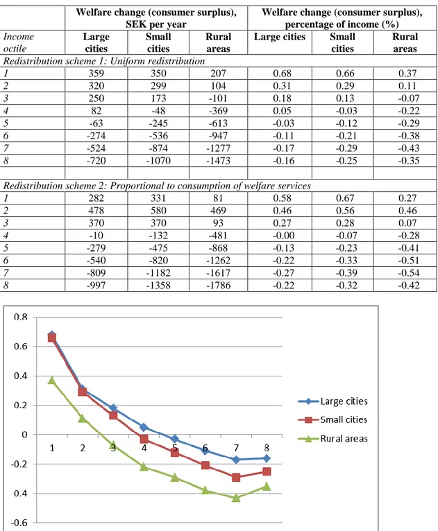
However, a complete analysis of the net welfare effect needs to take the use of revenues into account. As shown by e.g. Eliasson and Mattsson (2006) (analysing congestion pricing) and Bento et al. (2005; 2009), the net distributional effects can be radically different depending on how revenues are used. Therefore, Table 4 shows the net effect when the revenues from the fuel tax are redistributed according to two stylized redistribution schemes (ignoring transaction costs). The first redistribution scheme is a uniform redistribution to all adults. This can be thought to represent some form of public spending which is equal in monetary value for everyone. The second redistribution scheme emulates the distributional effects of a general increase in welfare services, such as education, culture, day care for children, health care and
15
nursing for elderly. We model this by assuming that tax revenues are distributed proportional to the group-specific average consumption of such welfare services (using figures from Statistics Sweden). Note that these services do not include welfare transfers such as unemployment benefits, health insurance or loss-of-income insurance, since these are paid for by the public insurance system.
Table 4. Net welfare change of fuel tax increase and revenue redistribution, by income octile and location type.
Welfare change (consumer surplus), SEK per year
Welfare change (consumer surplus), percentage of income (%) Income octile Large cities Small cities Rural areas
Large cities Small
cities
Rural areas Redistribution scheme 1: Uniform redistribution
1 359 350 207 0.68 0.66 0.37 2 320 299 104 0.31 0.29 0.11 3 250 173 -101 0.18 0.13 -0.07 4 82 -48 -369 0.05 -0.03 -0.22 5 -63 -245 -613 -0.03 -0.12 -0.29 6 -274 -536 -947 -0.11 -0.21 -0.38 7 -524 -874 -1277 -0.17 -0.29 -0.43 8 -720 -1070 -1473 -0.16 -0.25 -0.35
Redistribution scheme 2: Proportional to consumption of welfare services
1 282 331 81 0.58 0.67 0.27 2 478 580 469 0.46 0.56 0.46 3 370 370 93 0.27 0.28 0.07 4 -10 -132 -481 -0.00 -0.07 -0.28 5 -279 -475 -868 -0.13 -0.23 -0.41 6 -540 -820 -1262 -0.22 -0.33 -0.51 7 -809 -1182 -1617 -0.27 -0.39 -0.54 8 -997 -1358 -1786 -0.22 -0.32 -0.42
Figure 4. Welfare change, relative to income, of a fuel tax with flat revenue redistribution.
The table shows that the net effects of the fuel tax and any of the redistribution schemes are clearly progressive, regardless of location type. However, there are still clear differences across location types.
16
Distributional effects for the remaining three tax instruments are similar; results are presented in the Appendix, Table 15.
Summary of income distribution effects
To sum up, all the tax instruments are progressive over most of the income distribution. If the lowest and highest income outliers are included, they are just barely regressive. If revenue redistribution is taken into account, the progressivity becomes even more pronounced.
However, even if the instruments are generally progressive on average, this hides a considerable variation within income groups and types of location (large cities, small cities, rural areas). In rural areas and low income groups, the share of individuals who suffer substantial welfare losses is much higher than in large cities and high income groups. We hypothesize that this is what explains the common argument that car taxes hurt rural people and the poor disproportionately: even if car taxes are progressive on average, the share who suffer substantial welfare losses are much higher in lower income groups and rural areas.
If the tax instruments are meant solely as corrective taxes, internalizing external effects such as emissions, then we would argue that distributional effects are in fact essentially irrelevant, except for gauging transition costs. To the extent that they are fiscal instruments, however, distributional effects are very relevant: it is difficult to see why poor or rural people should contribute more than proportionately to the public purse.
5
DISTRIBUTIONAL EFFECTS ACROSS GEOGRAPHIC AREAS
Regional development trends, policies and debates in Sweden are similar to most developed countries. Decades of increasing urbanization and depopulation of sparsely populated areas have sparked long and lively debates about regional development and regional policy, and led to an active national policy for regional development, trying to revive or support sparsely populated areas, remote regions and rural areas. Transport and infrastructure are important components of this policy, and perhaps even more so in the public debate about these issues. The European Union have similar policies for regional development across the EU. The trends, arguments, policy measures (and results) would most likely be familiar in any developed country.
This means that distributional effects across geographic dimensions are important considerations in the transport policy debate. Indeed, this is arguably an even more important constraint on the design of transport policies than income equity effects, since the latter are somewhat easier to compensate through various social transfer systems or targeted discounts. Since governments spend substantial amounts on regional development policies, it is understandable that they may be reluctant to risk counteracting them with transport policies which may perhaps hurt rural or remote regions disproportionately.
The question is then how substantive this risk really is – that is, to what extent are rural, remote or sparsely populated regions actually worse affected by fuel and vehicle taxes than other locations? The difficulty with analysing this is that there are so many possible ways to disaggregate along geographic dimensions. However, in the Swedish debate (which is easy to translate to other national contexts), three main dimensions can be distinguished: rural vs. urban areas, metropolitan areas vs. medium/small cities, and northern vs. southern Sweden. We will analyse all these in turn, concentrating first on distributional effects of an increased fuel tax.
17
We use the definition of an “urban area” from Glesbygdsverket (the former Swedish Rural Development Agency): an area is defined as “urban” if houses are no more than 200 m apart and the area has more than 3000 inhabitants. Obviously, this means that “urban areas” exhibit large variation, as this will define quite a few small villages as “urban”. However, the definition is actually a reasonable distinction between “urban” and “rural”. 21% of Swedish adults live in rural areas. Excluding the three metropolitan regions (Stockholm, Gothenburg, Malmö), rural population shares do not vary much between counties – around 30% of the population live in rural areas all over the country, except in the three metropolitan areas. This is in fact probably surprising to most Swedes, since the northern parts of Sweden are very sparsely populated and the impression is probably that the northern half of the country is much more dominated by rural areas than the southern half. But in reality, most people live in urban areas in the northern half as well, just as in the southern part of the country.
Average incomes are slightly higher (7%) in urban areas. There is a strong correlation between accessibility to workplaces and average income, so more specific disaggregations increase this income difference.
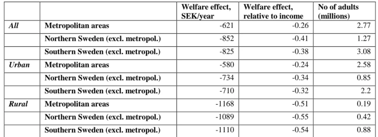
Table 5 shows the average welfare change of the fuel tax increase for three parts of the country – the metropolitan regions, northern and southern Sweden – and split by urban/rural area (Table 12 in the Appendix contains aggregate results as well as results split only by urban/rural). This reveals significant differences between urban and rural areas: the welfare losses in rural areas are 50-70% higher than those in urban areas. However, there are hardly any differences between rural areas in different parts of the country. Nor are there any differences between urban residents in northern and southern Sweden, excluding metropolitan areas. Apparently, the significant distinctions are only between metropolitan areas, other urban areas and rural areas – not between the southern and northern parts of the country.
Table 5. Welfare change from the fuel tax increase, split by part of the country and urban/rural area. Welfare effect, SEK/year Welfare effect, relative to income No of adults (millions)
All Metropolitan areas -621 -0.26 2.77
Northern Sweden (excl. metropol.) -852 -0.41 1.27
Southern Sweden (excl. metropol.) -825 -0.38 3.08
Urban Metropolitan areas -580 -0.24 2.58
Northern Sweden (excl. metropol.) -734 -0.34 0.85
Southern Sweden (excl. metropol.) -710 -0.32 2.2
Rural Metropolitan areas -1168 -0.51 0.19
Northern Sweden (excl. metropol.) -1089 -0.55 0.42
Southern Sweden (excl. metropol.) -1110 -0.54 0.88
Still, these distinctions hide considerable variation within metropolitan areas and within the group of “other urban areas”. This is revealed in Table 6, where locations are split according to whether they belong to a “central city” (the city which is the central point in its region), or whether they belong to a “satellite city” (cities which depend on a nearby central city for access to workplaces and specialized services). This shows that the important distinction is in fact not the size of the city but its functional role in the region. Central cities are actually more similar to metropolitan urban areas than to satellite cities, in terms of welfare effects of a fuel tax, despite being much smaller (> 60 000 inhabitants).
18
Table 6. Welfare change from the fuel tax increase, split by central city/satellite city. Welfare effect Welfare effect/income No of adults (millions)
All Central cities -690 -0.31 1.24
Satellites -856 -0.4 0.29
Urban Central cities -625 -0.28 1.09
Satellites -728 -0.33 0.2
Rural Central cities -1160 -0.52 0.15
Satellites -1138 -0.54 0.09
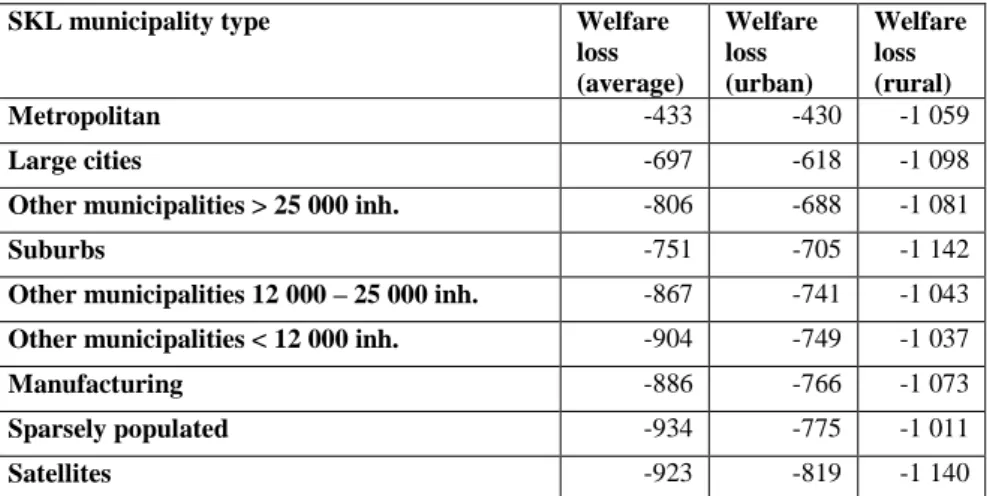
A similar classification of Swedish municipalities has been constructed by Sveriges Kommuner och Landsting (the Swedish Association of Local Authorities and Regions). Results according to this classification are shown in Table 7. The municipality types are sorted by increasing welfare loss in urban areas.
Table 7. Welfare loss from the fuel tax increase (SEK/year), split by SKL municipality classification and urban/rural area. Sorted by welfare loss in urban areas.
SKL municipality type Welfare
loss (average) Welfare loss (urban) Welfare loss (rural) Metropolitan -433 -430 -1 059 Large cities -697 -618 -1 098
Other municipalities > 25 000 inh. -806 -688 -1 081
Suburbs -751 -705 -1 142
Other municipalities 12 000 – 25 000 inh. -867 -741 -1 043 Other municipalities < 12 000 inh. -904 -749 -1 037
Manufacturing -886 -766 -1 073
Sparsely populated -934 -775 -1 011
Satellites -923 -819 -1 140
Again, we can conclude that the most significant difference is between urban and rural areas, and that effects for rural areas essentially do not vary across the country. After that, the most striking conclusion is that it is central cities who suffer the smallest welfare losses. Contrary to what one might believe, it is not primarily the size of the city that matters: even the relatively small central cities (down to 25 000 inhabitants) fare better than suburbs or satellites which may be both bigger, denser and/or belong to more populous regions. Comparing only the central cities (down to 25 000 inhabitants), it is true that size is indeed correlated with smaller welfare loss. But suburbs and satellites fare considerably worse, despite the fact that they usually belong to dense regions with large populations. All other municipalities fall between suburbs and satellites; the differences between urban areas in these other municipalities are comparatively small.
What is somewhat surprising with these results is, first, that the difference is so small between the suburbs in large/metropolitan regions and the small villages in remote and sparsely populated areas; second, that satellites are hit the hardest by far, despite usually giving a distinctly more “urban” impression. This would not be apparent from just a casual impression or superficial inspection of these urban areas. Satellites and suburbs usually have a distinct “urban feel” in their transport systems, land-use plans and architecture, not easily distinguishable from the “feel” in central cities of similar
19
size. But their different functional role in their respective region means that travel patterns are very different, with the obvious implications for welfare effects of car taxes.
The conclusion is that the most important geographic distinction is not “metropolitan regions vs. the rest” – it is the distinction between central cities and satellites/suburbs. The emergence of satellites and suburbs is to some extent a consequence of Swedish regional development policy. Macro-trends such as increasing specialization in jobs and services have tended to make agglomeration centres more attractive. Rather than facilitating the growth of the centres, and accepting that this must to some extent deplete surrounding cities, regional development policy has focused on facilitating long-distance commuting from these surrounding cities, turning them into suburbs and satellites where commuting distances are long and car mode shares high. There may be other benefits with this kind of regional policies, but it is clear that it constrains the possibilities to design policy instruments which reduce CO2 emissions.
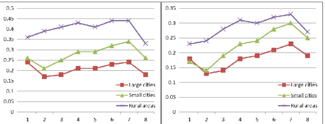
Turning to the other tax instruments, we divide municipalities into three types: urban areas belonging to large cities (the central city has more than 60 000 inhabitants), other urban areas (“small cities”) and rural areas, and split by income octile as well. The conclusions are essentially the same for all tax instruments, but the differences between income groups and location types are larger for the taxes on car use (fuel, kilometre) than for the ownership taxes (vehicle, purchase). Complete results are presented in the Appendix, Table 15.
Figure 5. Welfare loss relative to income from the fuel tax (left) and kilometre tax (right) split by income and geographical region. (The left diagram is the same as Figure 2 above.)
Figure 6. Welfare loss relative to income from the vehicle tax (left) and purchase tax (right) split by income and geographical region.
20
5.1 Summary of spatial distribution effects
Distributional effects across the geography are important constraints on policy design in most countries. We have shown that the most important differences are not between different geographical parts of Sweden, but between types of residential location: urban vs. rural, and between different functional types of urban areas. These dimensions are much more important for determining the effects of car taxes than for example whether an area is remote or sparsely populated.
The biggest difference in terms of welfare losses from car taxes is between urban and rural areas. Perhaps surprisingly, rural areas are affected similarly regardless of where in the country they are located – there is no difference between for example northern and southern Sweden – and all counties outside of metropolitan areas contain about the same share of rural residents.
The second biggest difference is between central cities and suburbs/satellites. Central cities, regardless of size, suffer much smaller welfare losses from car taxes than suburbs/satellites, even when comparing suburbs in metropolitan regions to small towns which still serve a central function in their region. In fact, the welfare losses of such suburbs are about the same size as those of “urban” areas (essentially villages) in very sparsely populated areas.
The third biggest difference is among central cities of different size: comparing only central cities with each other, it is clear that car use is negatively correlated with population, at least for larger cities. There are most likely several mechanisms behind this: for example, larger cities make attractive public transport more economically feasible; larger cities have worse traffic congestion; larger cities are denser, which tends to reduce travel distances (all else equal), and also tends to make walking/bicycling more competitive transport modes.
6
DISTRIBUTIONAL EFFECTS ACROSS LIFECYCLE GROUPS
In this section, we will study distributional effects across lifecycle groups. Defining such groups is necessarily somewhat arbitrary, especially since the number of groups cannot be too large. Led by a combination of data availability, previous research on travel behaviour and intuitive comprehensibility, we have opted for the classification illustrated in Figure 7. Each box is a lifecycle group, and the arrows indicate a few possible life trajectories as an individual goes from one group to another. “Young” is defined as less than 35 years, and “old” as more than 65 years. “Children” refers only to children living in the same household. “With partner” only includes married individuals and individuals living together with someone he/she has children in common with (the children do not have to live in the same household, though); other forms of relations are unfortunately not recorded in our data11.
11 In particular, from the data we cannot separate those who live alone from those who live together
21
Figure 7. Lifecycle groups, with a subset of possible life trajectories.
Table 8 shows the welfare effect of the fuel tax, split by lifecycle group and location type. Patterns across the lifecycle are similar regardless of location type. Some observations are obvious and rather expected. Having a partner increases car use, probably since costs can be shared. Having children increases car use considerably, except for young single parents, who do not use car more on average than young people without children (who may or may not have a partner). Middle-aged people use car much more than young people. Old people with partners use car about as much as middle-aged people without children. Old singles use car the least of all.
Table 8. Welfare effect of the fuel tax, split by lifecycle group and location type. Welfare change (consumer
surplus), SEK per year surplus), relative to income (%) Welfare change (consumer
Life cycle group Large
cities Small cities Rural areas Large cities Small cities Rural areas
Young no children -348 -556 -857 -0.17 -0.28 -0.45
Young with children
and partner -616 -807 -1137 -0.28 -0.38 -0.54
Young with children no
partner -341 -493 -877 -0.17 -0.24 -0.45
Middle-aged no
children -629 -891 -1349 -0.27 -0.40 -0.64
Middle-aged with
children and partner -1059 -1285 -1693 -0.38 -0.50 -0.69
Middle-aged with
children no partner -774 -1059 -1656 -0.30 -0.44 -0.72
Old with partner -623 -650 -830 -0.29 -0.36 -0.49
22
Table 9 shows analogous results for the differentiated purchase tax on new cars. Patterns are similar to the fuel tax effects, but differences across groups are smaller.
Table 9. Welfare effect of the purchase tax, split by lifecycle group and location type. Welfare change (consumer
surplus), SEK per year surplus), relative to income (%) Welfare change (consumer
Life cycle group Large
cities Small cities Rural areas Large cities Small cities Rural areas
Young no children -297 -446 -594 -0.14 -0.22 -0.31
Young with children
and partner -492 -580 -694 -0.22 -0.27 -0.32
Young with children no
partner -252 -317 -468 -0.12 -0.15 -0.24
Middle-aged no
children -532 -699 -865 -0.22 -0.31 -0.40
Middle-aged with
children and partner -851 -944 -1031 -0.30 -0.36 -0.42
Middle-aged with
children no partner -607 -730 -917 -0.23 -0.30 -0.39
Old with partner -674 -673 -729 -0.32 -0.37 -0.42
Old no partner -330 -374 -506 -0.16 -0.21 -0.31
6.1 Summary of distributional effects across lifecycle groups
The differences across lifecycle groups are the expected ones: having children increases car use, as does living with a partner, and young drive less than middle-aged. The patterns are similar regardless of location type, although the differences are more pronounced in large cities.
What may be surprising is that the differences are so large. The group with the highest car use (middle-aged with children and partner) drive between two and three times more (depending on location type – the difference is larger in large cities) than the groups with the lowest car use (young without children or without a partner; we can exclude old people without a partner from this discussion since they are special in other respects). This is not primarily an income effect, which can be seen from the welfare losses relative to income. The welfare loss relative to income for the group with highest car use is still more than 50% higher than for the young groups.
7
CONCLUSIONS
Taxes on cars and fuel are important both as fiscal and policy instruments. However, their distributional effects are often viewed as constraints on their design. There are widespread concerns that taxes on cars and fuel may have unwanted distributional effects, such as being regressive or hurting remote or rural areas more than urban areas. We analyse four tax instruments: an increase in fuel tax, a new kilometre tax, an increased CO2-differentiated vehicle tax, and a new CO2-differentiated purchase tax on
new cars. The analysis is based on Swedish administrative registers containing all private cars in Sweden 2011.
Our results show that all analysed tax instruments are progressive over most of the income distribution. If the lowest and highest income outliers are included, they are just barely regressive. However, there is considerable variation within income groups and types of location (large cities, small cities, rural areas). In rural areas and in low
23
income groups, the share of individuals who suffer substantial welfare losses is much higher than in large cities and high income groups. This may explain the common assertion that car taxes hurt rural people and the poor disproportionately: even if car taxes are progressive on average, the share who suffer substantial welfare losses are much higher in lower income groups and rural areas. If the tax instruments are meant solely as corrective taxes, we argue that distributional concerns are actually not very relevant (except for considering transition costs when people adapt to changes in transport costs), since prices are (for good reasons) usually independent of income; problems with inequitable income and wealth distributions are normally handled by tax and welfare systems. If the purpose is fiscal, however, distributional concerns are very relevant: it is difficult to see why poor or rural people should contribute more than proportionately to public tax revenues. In reality, fuel and vehicle taxes usually have both fiscal and corrective purposes, and figuring out the relative importance of these purposes may be nearly impossible; at least, different analysts can apparently reach different conclusions regarding to what extent current taxes can be motivated by “corrective taxation” arguments12.
Distributional effects across the geography are important constraints on policy design in most countries. In our analyses, the most important distinctions are, in decreasing order of importance, 1) between urban13 and rural areas 2) between central cities and
satellites/suburbs, and 3) between central cities of different sizes. These dimensions are much more important for determining the effects of car taxes than for example whether an area is remote or sparsely populated. Rural areas are affected similarly regardless of where in the country they are located – there is no difference between for example northern and southern Sweden – and all counties except metropolitan areas contain about the same share of rural residents. Central cities, regardless of size, suffer much smaller welfare losses from car taxes than suburbs/satellites, even when comparing metropolitan suburbs to small towns which nevertheless serve as centres of their respective region. Welfare losses of metropolitan suburbs are in fact in the same magnitude as those of “urban” areas (essentially villages) in very sparsely populated areas. For central cities, car use is negatively correlated with population size, at least for larger cities.
We conclude that for urban regions (which also includes villages down to 3 000 inhabitants), the real distinction in terms of distributional effects of car taxes is neither between metropolitan areas and smaller cities, nor between northern and southern Sweden – it is between central cities and suburbs/satellite cities. How an urban region is affected by a change in car taxes is hence determined more by its functional role in its region than its size or geographical location. The growth of satellites and suburbs is to some extent a consequence of a complex set of policy deliberations with the ultimate aim to stimulate development and employment in rural and sparsely populated regions, e.g. by encouraging long-distance commuting. Such policies may yield other kinds of benefits, but it is clear that it constrains the possibilities to design policy instruments which reduce CO2 emissions. Stimulating long distance commuting may be
12 For example, the current Swedish CO
2 tax on fuel is around 110 €/ton CO2, which is considerably
higher than for example the price of CO2 in the European Emission Trading Scheme. Some
commentators argue that this shows that the tax is too high from a climate policy perspective, and would hence argue that the purpose is mainly fiscal; other commentators, however, argue that the tax should be considerably higher for climate policy reasons.
13 An urban area is defined as a contiguous area where distances between houses do not exceed 200 m,
and the total number of inhabitants in the area exceeds 3000. Hence, this includes quite a few rather small villages.