Modeling Product Line Variability in the Rail Vehicle Domain

School of Innovation Design and Engineering

V¨

aster˚

as, Sweden

Thesis for the Degree of Master of Science (60

credits) in Computer Science with Specialization in

Software Engineering — 15.0 hp — DVA423

MODELING PRODUCT

LINE VARIABILITY IN

THE RAIL VEHICLE

DOMAIN

Stefan Bogicevic

sbc17003@student.mdh.se

Examiner: Federico Ciccozzi

M¨

alardalen University, V¨

aster˚

as, Sweden

Supervisor: Eduard Enoiu

M¨

alardalen University, V¨

aster˚

as, Sweden

May 31, 2018

Abstract

Software Product Line Engineering (SPLE) is a development ap-proach used for handling large amounts of variants in software sys-tems. The idea behind this approach is to exploit reusability of various similar and diverse products. Reusable products have various common-alities and differences that can be exploited, and to do so, developers need to define those differences (i.e., variabilities) within them. Vari-abilities can occur at different abstraction levels, through whole prod-uct lifecycle and developer need to handle it through the whole process. To address this problem at the architectural and requirement level, we used pure::variants, a leading variant-management commercial tool, to model variability within requirements in the railway domain. With this tool, we explicitly define a process on how to design a variability model that could be used to model several aspects of requirement vari-ability, which can be reused again in the future, for the requirement engineering. We propose an approach for engineers to automatically generate models from requirement documents and then with the use of pure::variants functions, create various aspects which are then further transformed into feature models. Finally, the results of this trans-formation made possible the identification between core and variant features presented in these requirements making it easy to define what parts of the software are project specific and what are common for all generated models. Our results indicate that variability modelling using the pure::variants tool is applicable for requirement variant handling in the railway domain.

Table of Contents

1.2 Goal and Problem Statement . . . 9

2 Background 10 2.1 Software Product Line Engineering . . . 11

2.2 Variability . . . 13

2.3 Feature Model . . . 14

2.3.1 Variants . . . 16

2.3.2 Variation Points . . . 17

2.4 pure::variants Tool . . . 18

2.4.1 Variant Management Perspective . . . 20

2.4.2 Feature Models in pure::variants . . . 20

2.4.3 Family Models . . . 23

2.4.4 Transformation . . . 25

2.5 Related Work . . . 25

3 Research Process 29 4 A Method for Variability Requirement Transformation and Modelling 32 4.1 System Under Study . . . 32

4.2 Requirements Analysis . . . 33

4.3 Transformation and Implementation Approach . . . 35

4.4 Basic Requirements Transformation to Feature Model . 35 4.4.1 Comma Separated Values (CSV) Transforma-tion/Conversion . . . 36

4.4.2 Generating Feature Model . . . 39

4.4.3 Variant Description Models . . . 39

4.4.4 Variants Modeling . . . 40

4.5 Transformation of Detailed Requirement Functions to Feature Models . . . 43

4.5.2 Relations and Attributes . . . 47

4.5.3 Feature Model . . . 48

4.5.4 Attributes Calculation Rules . . . 48

5 Method Evaluation 54 5.1 Final Transformation Results . . . 54

5.1.1 Basic Transformation . . . 54

5.1.2 Detailed Transformation . . . 54

5.2 Model and Variant Analysis . . . 58

5.2.1 Selection State Analysis . . . 58

5.2.2 Similarity matrix . . . 61 6 Conclusion and Future Work 63

List of Figures

2.1 Train Feature Model . . . 12

2.2 Feature modeling approaches . . . 16

2.3 Overview of family-based software development with pure::variants [1] . . . 19

2.4 Initial layout of the Variant Management Perspective . 21 2.5 A simple Feature Model of a car . . . 22

2.6 Basic structure of Feature Models [1] . . . 23

2.7 Basic structure of Family Models [1] . . . 24

2.8 Sample Family Model . . . 25

2.9 pure::variants transformation process . . . 26

2.10 Product line adoption strategies [2] . . . 27

3.1 Research process cycle. . . 30

3.2 Our research process overview . . . 30

4.1 Bombardier TCMS model . . . 33

4.2 Transformation and Implementation Approach . . . 36

4.3 Requirement to feature mapping . . . 37

4.4 Mapping of requirement information to CSV file . . . . 38

4.5 Generated feature model . . . 39

4.6 Feature model structure based on requirements func-tionality . . . 40

4.7 Feature model functions and their requirements . . . . 40

4.8 Feature model functions and their requirements . . . . 41

4.9 Connecting the feature model to configuration space . . 41

4.10 Variant description models for project A and B . . . . 42

4.11 Process of selecting required features . . . 42

4.12 Feature Model with added relations and attributes . . . 51

4.13 Rule 1: Location Confirmed Flag . . . 51

4.14 Rule 2: Location Mismatch . . . 52

4.15 Rule 3: Direction of travel . . . 52

4.16 Rule 4: Current Location . . . 52

4.17 Feature model with calculations and attributes values . 53 5.1 Final model for Door A . . . 55

5.2 Final model for Door B . . . 56

5.3 Final transformation results for detailed feature model 57 5.4 Final transformation results after changing attribute value . . . 58

5.6 Selection state cluster: variant functionality . . . 61 5.7 Similarity matrix . . . 62 5.8 Compare Model . . . 62

List of Tables

2.1 Element variation types and its icons . . . 21

4.1 Example of requirements used . . . 34

4.2 Relations between requirements . . . 48

4.3 Requirement Attributes . . . 49

Glossary

SPLE Software Product Line Engineering PLE Product Line Engineering

MITRAC Modular Integrated TRACtion system TCMS Train Control Management System

SPL Software Product Lines

FODA Feature-Oriented Domain Analysis UML Unified Modeling Language

VDM Variant Description Model CCU Computer Control Units XLSL Microsoft Excel

CSV Comma Separated Values

1

Introduction

The need for creating reusable products increased exponentially in the past two decades due to the sheer number of product variants needs of engineering complex software. The ability to create a large number of product targeting specific customer needs, decreased total cost of the product development and increased the revenue of companies are all critical for applying scalable methods for handling variability. Making a customized product that will match with customer’s desire enables companies to release a mass number of products to the market in a more efficient way. This process requires some management that will handle variations and complexity inside this similar product types. This thesis is focused on studying the use of variability modelling explicitly targeting the rail-vehicle domain.

In Section 2 we explain what is Product Line Engineering (PLE) and what are main development issues with the mass creation of prod-ucts. Besides, we will introduce variability inside PLE and what tools and methods are used to handle it. After, we will describe feature modeling and point out its advantages and how it is used for variabil-ity management and to enhance the development process. In the end, we will present a variability management tool (i.e., pure::variants) that we used in this thesis.

In Section 3, we explain what research method is used in this thesis, and we propose our research goals. In Section 4 we will describe what the properties of the system that we will study are. The system under study is the Bombardier Transportation’s Modular Integrated TRAC-tion system (MITRAC), Train Control Management System (TCMS), and we will explain how TCMS controls various functions. In our case, we focus on the door opening functionality for two different projects. In the end, we will describe the variability modelling process. Finally in Section 5 we present the results of our research and evaluate this process regarding applicability.

1.1

Motivation

As the use of software deals with various problems and the capabilities of complex products are getting more and more popular in the rail-way domain, handling of product variants is getting more and more complex as well. Complex systems mean integrating more and more software products within the system, and this indicates more

varia-tions between them. More variavaria-tions mean more complex systems, and one can say that complexity in railway software development [3] is due to this high variability. To manage the variability of the pro-duced software, a cost-effective development process [3] needs to be used. Software Product Lines (SPL) are trying to solve this issue. Var-ious works have been published [4], showing that the SPL approach is a successful solution for handling the complexity and variability of the software developed in different domains, in this case, rail-vehicle domain.

Variability is the ability of a software system or software artifact (e.g., component) to be adapted so that it can be used in a specific context [5]. During past decade the need for creating dynamic systems that can be adjusted to modifications increased exponentially. Static systems that require extensive and expansive editing of existing code are no longer suitable for contemporary software development [6], and therefore variability becomes a fundamental property of many sys-tems. Variability gives more knowledge about softwares structure and behavior and its ability to readjust its processes to the different situ-ations. This is achieved using variations points and enabling different variants [7] to be chosen at these variation points. Use of variability in software systems reassures that the system can easily be adapted to the adjustments and [7] ”to facilitate the reusability of software systems or individual software artifacts”.

Software Product Line Engineering (SPLE) allows and bring new ways to develop an extensive range of software products [8] which can be built faster, cheaper and better. This wide range of products that are developed with the software products lines is hard to maintain and to support different, individual customers or address entirely different market segments. That is where variability steps in, as a leading concept in the SPLE. Modeling this variability should enable more natural configuration of different parts of rail vehicle systems, which will further improve the development effectiveness, resulting in the reduction of cost for the whole development.

1.2

Goal and Problem Statement

The past decades have witnessed an increasing research effort on dif-ferent approaches in product line engineering in difdif-ferent domains [9]. However, there are a few studies that evaluate these techniques in

in-dustrial practice with even fewer studies targeting the railway safety-critical domain. In the context of automotive software, model-based techniques have been proposed [10] for representing the solution by using a single model with commonalities and differences.

The primary objective of this thesis is to investigate and document the use of product line engineering through variability modeling. In the end, we would like to provide an approach to engineers on how to explicitly model the variability within the requirements on the archi-tecture level in the railway domain. The results of the thesis should indicate the advantages or disadvantages of implementing model-based variability in industrial practice. The overall objective of this thesis is to design a variability model that could be used to model several aspects of variability. This designed variability model is to be used during the design of a software platform project to define which parts of the software will be project specific, which ones will be in common for the platform projects, and how the project specific and common software will be linked together into an overall project software. The goal is to present proposals for how to model the variability so that this provides a structure for the code implementation.

The tool that has been used in this thesis is pure::variants, a commercial tool for variant and variability management for product lines. The pure::variants approach uses extended feature models [11] for modeling of the problem domain and support managing of vari-ability in every step of product line engineering. The goal is to show how reusable product line architecture can be build by using modeling capabilities provided by pure::variants.

In the end, the thesis aims to explore the use of a tool for model-based variability, define its advantages and disadvantages and explic-itly design a model that could be used to model several aspects of variability.

2

Background

PLE [12] is a widely used method for the efficient development of large portfolios of products. This method is based on the fact that prod-ucts are built from a collection of artifacts that have been specifically designed for use across the portfolio.

To take into account for differences among the products, some adaptations of the artifacts are usually needed. These adaptations

should be planned before development and made available for the en-gineers and architects to use without compromising existing properties of the core artifacts. Managing this may result in adding unnecessary variability [13], implementing variations more than once, selecting in-compatible variation mechanisms, and missing required variations.

Variability is one of the most critical concepts of software prod-uct lines. Variability enables software system or software artifacts to be re-configured, broaden and reshaped to use in different contexts. Variability allows different variations of software products to be made, facilitating and enhancing software development process. As the prod-uct line grows and evolves, the need for variability increases, and man-aging the variability grows increasingly difficult.

The most popular technique to model variability of products of a product line is feature modeling [11]. In the feature modeling, vari-ability is modeled from the perspective of product features. Features present abstract concepts [14] which are supporting communication within different stakeholders of a product line. Figure 2.1 shows an example of using feature model of a train product line.

Variability modeling intends to create and manage many variants of a product, also known as mass customization1. Variability mod-eling is regarded as the enabling technology for delivering a wide variety of software systems of high quality in a fast, consistent and comprehensive way. The key is to build a base on the commonalities and efficiently express and manage the variability of the systems [15]. SPLE intends to develop software-intensive systems using this mass customization. There is various work already proposed for product line variability modeling [16] [8] [7].

2.1

Software Product Line Engineering

PLE enables the creation of an extensive portfolio of related products exploiting their similarities while handling their differences.PLE uses products lines to achieve this. A product line is a collection of closely related products with variations in their supported features [17]. Ris-ing demand in the industry for the individualized products marked the beginning of mass customization, which included giving customers matching products that meet their requirements. Mass customization

1_{”Mass customization is the large-scale production of goods tailored to individual customers’}

Figure 2.1: Train Feature Model

allows users to have an individualized product. For the company, it means having a high tech involvement which leads to higher prices for those products. This effect was undesirable, and that lead to in-troducing platforms for different product types. In those platforms, plans were made before production, deciding which part will be used in different product types. Platforms allowed companies to offer a more extensive variety of products and to reduce costs for them. Cost reduction was one of the main advantages of product line engineering, together with enhancement of quality and reduction of time to market. Indifferent to product lines, SPLE is using software engineering methods, tools and techniques to enable an extensive range of soft-ware products to be built faster, cheaper and better. The benefits of using mass customization that are mentioned above exponentially de-creased the maintenance cost and resulting in an inde-creased propensity toward the use of product lines [18]. SPLE offer practical strategies to develop families of products [18]. This wide range of products that are developed with the software products lines is hard to maintain, together with supporting the different, individual customers or to ad-dress entirely different market segments. The members of the product family are connected with the familiar concepts, but they also consist of different properties that make them unique. Presence of this vari-ation inside product family distinguishes the main difference between

software product line engineering and conventional software engineer-ing. Thus successfully managing this commonality and variability in SPLE is a vital issue, and SPLE approach has proven to be a successful solution for handling it [4].

2.2

Variability

As a critical discipline in SPLE, variability represents a fundamen-tal aspect of the software. It is the ability to create, extend, change system variants through customization depending on the specific con-text [5]. Although variability has been mostly used and studied in software product lines, it can also be found in some other areas, like context-aware software [19] or software ecosystems [20]. Virtually any successful software faces eventually the need to exist in multiple vari-ants [21]. The concept of variability can be referred as a process of defining required features that system needs to include [17] and all the variation of those features that can be configured.

Introducing variability means introducing structural complexity in all areas of software engineering and using various tools and method to deal with it efficiently. The variable system can be referred as a set of systems engineered simultaneously; thus requirements, archi-tecture, code and tests [21] are more complex than in single-system engineering. This means that if a developer wants to understand a par-ticular system variant he needs to analyze only the relevant parts of requirements. Variability-aware methods and tools leverage the com-monalities among the system variants while managing the differences effectively [17].

Using feature models [11], hierarchically composed declarations of common and variable features and their [2] dependencies, Variability modeling at the requirements level can be used for visual representa-tion of a variable system which will facilitate explaining the system and its evolution to all stakeholders, technical and nontechnical ones. At this system level, features can be used as a visual demonstration of all requirements enabling all stakeholders to understand the system, its variability, and its evolution [22].

In the article [7], authors pointed out several problems with man-aging variability within SPL:

• Knowledge gap: While designing and implementing large-scale systems, very often a knowledge gap appears between domain

ex-perts and engineers that implement the system. High-level design of the domain experts usually follows with the low-level implemen-tation of engineers, that can result in inconsistent implemenimplemen-tation. • Traceability: To fully understand the system variability, system architecture must be designed in a way that all the artifacts can be easily traced from the high-level design down to the implemen-tation level.

• Dispersed variation points: In requirements level, the feature can have numerous variation points that reside in different parts of the final model. Multiple features can affect multiple variation points, resulting in difficulties while identifying what code is dependent on a feature.

2.3

Feature Model

Feature-oriented approach [11] offers an effective way of modeling and managing commonality and variability within product families. Over past two decades, Feature Modeling has been widely accepted by the software reuse and the SPLE communities as a means for modeling a commonality and variability of a product line. Features are abstract concepts, and therefore they can be used for establishing communi-cation among diverse stakeholders of a product line, and it is easy to express commonality and variability of product lines in terms of features [14]. Feature Modeling has been used to visualize features, their composition relationships, and variability relationships among features. Informally, features are key distinctive characteristics [23] of a product. Different domain analysis methods use a different meaning for the term feature. Feature-Oriented Domain Analysis (FODA) [11] defines a feature as a ”prominent and distinctive user-visible charac-teristic of a system”. Notation used in this research follows the FODA definition. As it is mentioned before, features are a distinct concepts or characteristics that are visible to various stakeholders, but on the other hand it is important to note that the purpose of feature mod-eling should be laid in identifying commonality and variability in a domain rather than differentiating concepts from features [23]. Also, it is important to distinguish features from other conceptual abstrac-tions (function, object, and aspects). Those abstracabstrac-tions are mainly used for describing internal parts of the system, while features are

ex-ternal characteristics that vary from one product to another. Thus the focus of feature modeling must be on identifying external characteris-tics of products (features) regarding variability, rather than describing all products details (internal parts). Those parts can later be derived from the understanding of commonality and variability of products.

Feature Models are used to describe the functionality of a domain. A functionality represent products properties which can be a require-ment or component within product architecture. Feature Models can visually describe both similarities and differences of all the products in a product line and draws a line between a common and variant feature of it. There are several modeling notations [24] that can be found in the literature. One of the first notation, FODA proposed by Kang [11] uses a graphical representation (feature model) to show the identified features. Some FODAs extensions can be found in the liter-ature, such as Feature-Oriented Reuse Method (FORM), Generative Programming Feature Tree (GPFT), Van Gurp and Bosch Feature Diagram (VBFD) and more. Like it is mentioned, there are multiple notations for describing feature models and for purpose of this research we use FODA since it is simple, clear, and expressive. Four types of fundamental relations exist between features: mandatory, optional, alternative, and OR. Common features among different products are modeled as mandatory features, while different features among them may be optional or alternative. A mandatory feature indicates that the child feature in this relation is always present, whenever its par-ent feature is prespar-ent. Optional features represpar-ent selectable features for products of a given domain and alternative features indicate that no more than one feature can be selected for a product. OR feature represents that at least one of the sub-features must be selected. To capture the structural relation between features, feature diagram is used. Feature diagram is a graphical presentation of features, using AND/OR hierarchy. Figure 2.1 describes a simple feature model in the domain of train configuration using FODA.

Five types of relationship are represented in this diagram. Ex-cept for the four of fundamental relations, there is also dependency relation: required, which indicate that one feature functionality de-pends on the existence of another. In this example optional feature electric battery required a battery feature for its functionality. In the model, train consists of mandatory features, engine, doors, and bogie while also having optional features that can be chosen like air

con-ditioning condenser, battery or auxiliary inverter meaning that some train can have those features while others may not. A child feature in an alternative relation may be present in a product if its parent feature is included. In this model, engine is a mandatory feature, and it must be included, and children of this feature are connected with the alternative relationship which indicates that it should be either petrol OR diesel OR electric gas but not all of them or even two of them. On the other hand, the child feature in an ORrelation may be present in a product if its parent feature is included, but at least one feature of the set of children should be present. Extra functionality can air conditioning condenser AND/OR battery AND/OR auxiliary inverter. This means that train can have multiple extra functionalities or at least one of them.

Since its introduction in 1990, in response to the changing need of market and extensive growth of the industry, substantial improve-ments have been made thus making feature models more expressive. In Figure 2.2 you can see the various evolution of feature models thought years.

Figure 2.2: Feature modeling approaches 2.3.1 Variants

Variants represent differences among similar products. The manda-tory features can be decomposed into alternative features and alter-native features complete mandatory depending on the system archi-tecture. In figure 2.1 the alternative features are the features that are present at the abstraction level below the mandatory features. Al-ternative and optional features can have a dependency on the other

features, meaning the existence of one feature include or exclude the other. In figure 2.1 the selection of electric battery includes a se-lection of battery functionality, while the sese-lection of diesel excludes selection of petrol and diesel because only one of them can be included in a vehicle variant. The OR relationship modern features that don’t have dependencies on each other. For example, a train can have both the battery, the air conditioning condenser and an auxiliary inverter features selected as extras in a vehicle.

2.3.2 Variation Points

Reusability and flexibility have been the driving forces behind the development of SPLs. With those techniques, we can delay certain design decisions to a later point in the development [25]. In SPL, the architecture of a system is designed early, but until the actual product implementation, we do not have all the details of its implementation. Those delayed design decisions are called variation points and they can be introduced at various levels [25] of abstraction:

• Architecture Description - Typically the system is described us-ing a combination of high-level design documents, architecture description languages, and textual documentation.

• Design Documentation - Describing system using various Unified Modeling Language (UML) notations, together with textual doc-umentation.

• Source Code

• Compiled Code - Compile source code using the compiler.

• Linked Code. During the linking phase, the results of the compi-lation phase are combined.

• Running code - During execution, the linked system is started and configured.

Variation points mostly accommodate variability at the architec-tural level. ”They are locations in software artifacts where variability occurs” [24]. Variation points describe where variations occur between different variants of a product. They describe what the selection of variants was and how they relate to each other. Therefore optional and

variable features and represented with the usage of variation points during software implementation [17].

In Figure 2.1 at the start of the development, we can see that all possible systems can be built. Each step further into the development confine one set of possible products until there is only one system left. Variation points aids in delaying this restriction and with it, they enable having greater variability in each step of the development. As mentioned above, variability can be introduced at various levels of abstraction. In [25], authors distinguish three states for a variation point in a system:

• Implicit - Having variability introduced at a particular level of abstraction indicates that at higher levels of abstraction this vari-ability is also present.

• Designed - Variation points can be designed as early as the archi-tecture design.

• Bound - Whole purpose of designing the variation points is so it can be bound later with a specific variant.

In addition, terms open and closed are also used in relation to abstraction level. Open variation point means that new variants can still be added to the system. On the other hand, closed variability means that there is no way to add variation.

2.4

pure::variants Tool

Pure::variants2 is one of the most well know tools commercially avail-able for variant and variability management of product lines. The pure::variants approach uses extended feature models [11] for mod-eling of the problem domain and support managing of variability in every step of product line engineering. pure::variants, with the set of integrated tools, supports each phase of the software product-line development process. pure::variants can also be used as an open frame-work and integrate with other tools that are used for different aspect of software development such as requirements management systems, object-oriented modeling tools, configuration management systems,

bug tracking systems, code generators, compilers, UML or SDL de-scriptions, documentation, source code, etc.

Activities and models that are vital for family-based software de-velopment and that are used in pure::variants are presented in Figure 2.3. For representing the problem domain for Product Line infrastruc-ture, pure::variants uses Feature Models. Family models are used for implementing solution domain. Those two model are complementary to the two models used for Application Engineering, i.e. the creation of product variants. The Variant Description Model (VDM) is used for representing a single problem from the problem domain. VDM contain all the selected feature set and associated values that display one product. The Variant Result Model describes a single concrete solution drawn from the solution family.

Figure 2.3: Overview of family-based software development with pure::variants [1]

For the purpose of this research, we used pure::variants eclipse ex-tension. The pure::variants Eclipse plug-in extends the Eclipse IDE to support the development and deployment of software product lines. Using pure::variants, a software product line is developed as a set of integrated Feature Models describing the problem domain, Fam-ily Models describing the problem solution and Variant Description Models (VDMs) specifying individual products from the product line. Feature Models describe the products of a product line concerning the features that are common to those products and the features that

vary between those products. Each feature in a Feature Model repre-sents a property of a product that will be visible to the user of that product. These models also specify relationships between features, for example, choices between alternative features. Feature Models are described in more detail in Section 2.4.2.

Family Models describe how the products in the product line will be assembled or generated from pre-specified components. Each com-ponent in a Family Model represents one or more functional elements of the products in the product line, for example, software (in the form of classes, objects, functions or variables) or documentation. Family models are described in more detail in Section 2.4.3

2.4.1 Variant Management Perspective

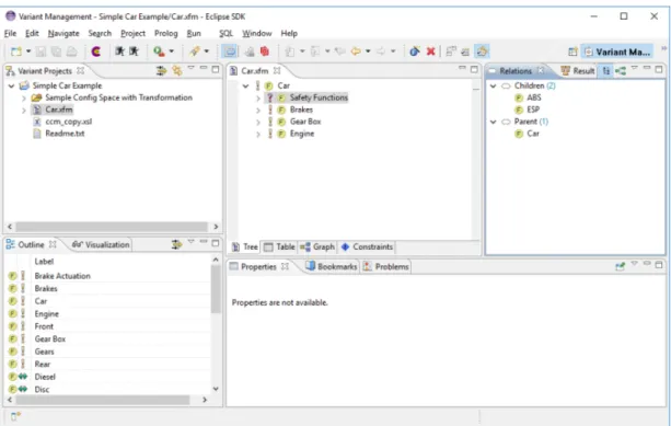
Figure 2.4 shows the basic layout of the pure::variants tool perspective integrated into the eclipse. On the left side, you can see project ex-plorer showing all active projects, in the middle is main pure::variants editor window where can be seen all the feature and family models opened in the tool, together with a various transformation that tool can offer. On the right side, there is result window which shows the results of specific transformation which was used upon selected feature model.

2.4.2 Feature Models in pure::variants

As discussed in Section 2.3, Feature Models are used to express com-monalities and variability within the system efficiently. A feature is a property of the problem domain that is relevant with respect to com-monalities of, and variation between, problems from this domain. Be-ing relevant means that there is a certain interest for explicit represen-tation of the given feature (property). This interest comes from differ-ent stakeholders that are involved in the developmdiffer-ent process. What is relevant thus depends on the stakeholders. Different stakeholders may describe the same problem domain using different features. Fea-ture relations can be used to define valid selections of combinations of features for a domain. These relations are represented with a feature tree. In this tree the nodes are features, and the connections between features indicate whether they are optional, alternative or mandatory. Table 2.1 explains these terms and shows how they are represented in feature diagrams. Additional constraints can be expressed as

restric-Figure 2.4: Initial layout of the Variant Management Perspective Table 2.1: Element variation types and its icons

Short name Variation type Description Icon mandatory ps:mandatory A mandatory element is implicitly

selected if its parent element is selected. optional ps:optional Optional elements are selected independently. alternative ps:alternative

Alternative elements are organized in groups. Exactly one element has to be selected

from a group if the parent element is selected. or ps:or

OR elements are organized in groups. At least one element has to be selected

from a group if the parent element is selected.

tions, element relations, and model constraints. Possible restrictions could allow the inclusion of a feature only if two or three other features are selected as well, or disallow the inclusion of a feature if one of a specific set of features is selected.

Figure 2.5 shows the basic view of feature model inside pure::variants eclipse extension. The Outline view (lower left corner) shows config-urable views of the selected Feature Model and allows fast navigation

to features by double-clicking the displayed entry. The Properties view in the lower middle of the Eclipse window shows properties of the cur-rently selected feature. The Table tab of the Feature Model Editor (shown in the lower left part) provides a table view of the model. It lists all features in a table, where editing capabilities are similar to the tree (e.g., same context menu, cell editors concept); it allows free selection of columns and their order.

Figure 2.5: A simple Feature Model of a car

The Details tab of the Feature Model Editor provides a differ-ent view on the currdiffer-ent feature. This view uses a layout and fields inspired by the Volere requirements specification template to record more detailed aspects of a feature. The Graph tab provides a graphi-cal representation of the Feature model. It also supports most of the actions available in the feature model Tree view. The Constraints tab contains a table with all constraints defined in the model supporting full editing capabilities for the constraints.

In Figure 2.6, we show the principle structure of a pure::variants Feature Model as UML class diagram. A problem domain consists of any number of Feature Models. A Feature Model has at least one feature.

Figure 2.6: Basic structure of Feature Models [1] 2.4.3 Family Models

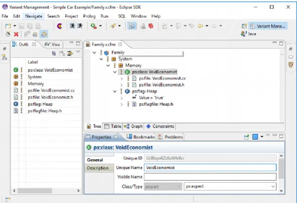
The Family Model describes the solution family regarding software architectural elements. Figure 2.7 shows the basic structure of Fam-ily Models as a UML class diagram. Both models are derived from the SolutionComponentModel class. The main difference between the two models is that Family Models contain variable elements guarded by restriction expressions. Since Concrete Component Models are derived from Family Models and represent configured variants with resolved variabilities there are no restrictions used in Concrete Com-ponent Models. The comCom-ponents of a family are organized into a hierarchy that can be of any depth. A component (with its parts and source elements) is only included in a result configuration when its parent is included and any restrictions associated with it are fulfilled. For top-level components only their restrictions are relevant.

Components: A component is a named entity. Each component is hierarchically decomposed into further components or into part el-ements that in turn are built from source elel-ements.

Parts: Parts are named and typed entities. Each part belongs to precisely one component and consists of any number of source ele-ments. A part can be an element of a programming language, such as a class or an object, but it can also be any other essential element of the

Figure 2.7: Basic structure of Family Models [1]

internal or external structure of a component, for example, an inter-face description. pure::variants provides many predefined part types, such as ps:class, ps:object, ps:flag, ps:classalias, and ps:variable. The Family Model is open for extension, and so new part types may be introduced, depending on the needs of the users.

Source Elements: Since parts are logical elements, they need a corresponding physical representation or representations. Source el-ements realize this physical representation. A source element is an unnamed but typed element. The type of a source element is used to determine how the source code for the specified element is generated. Different types of source elements are supported, such as ps:file that merely copies a file from one place to a specified destination. Some source elements are more sophisticated, for example, ps:classaliasfile, which allows different classes with different (i.e., aliases) to be used at the same place in the class hierarchy. The actual interpretation of source elements is the responsibility of the pure::variants transforma-tion engine. To allow the introductransforma-tion of custom source elements and generator rules, pure::variants can host plug-ins for different transfor-mation modules that interpret the generated Variant Result Model and produce a physical system representation from it. The semantics

of source element definitions are a project, programming language, and/or transformation-specific. Figure 2.8 shows an example of the family model.

Figure 2.8: Sample Family Model 2.4.4 Transformation

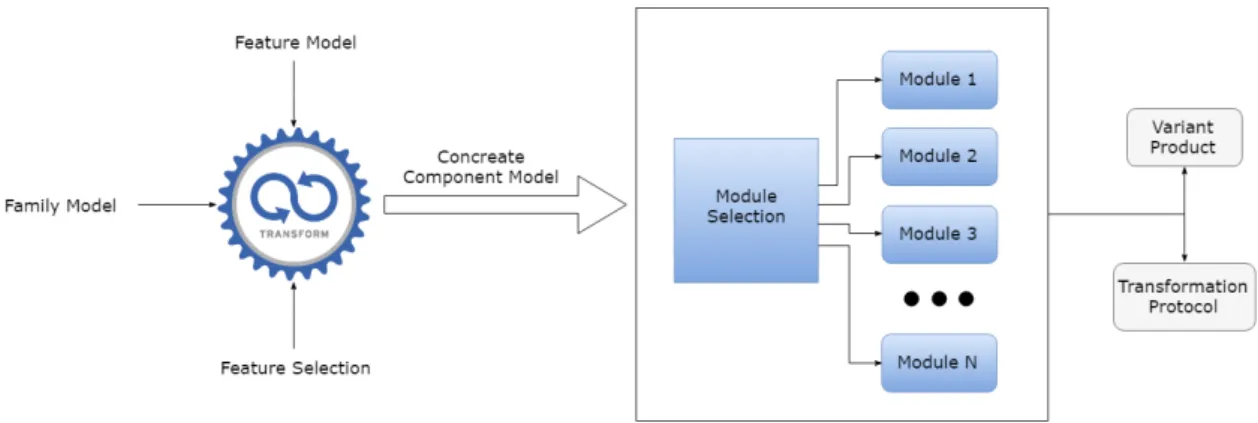
Figure 2.9 shows the basic process of creating variants with pure::variants. After producing different models, all steps that remain are automat-ically performed. The responsibility of the developers is to provide the feature and family models. After providing the models, features can be selected. Further processing is performed in two steps. At first pure::variants analyzes the different models. The result is a construc-tion plan from which the customized component of the final product is derived in a second step.

2.5

Related Work

The industry is often using software product line engineering to handle convoluted variability. Variability modeling is using models to provide

Figure 2.9: pure::variants transformation process

an abstraction of variabilities inside similar products types (families) allowing engineers to plan the system evolution.

Over the past two decades, various variability modeling techniques have been proposed and introduced into the industry and academia, with a large number of different notations and tools available. Even so, just a few studies present the industrial application of such tech-niques and their empirical evaluation. This is, in most part, due to the lack of empirical data gathered from these studies. Without the proper evaluation, the progress of such techniques can stagnate the application of such techniques in practice.

In order to gain more empirical data, researchers have studied the application of variability modelling [2] [8]. A Survey [2] conducted in 2013, mainly focused on extracting the attitudes towards variability modeling and its perceived benefits show that most companies that are involved with automotive industry apply variability modeling for development of their software. Automotive domain leads the group of the application domains in which companies are applying variabil-ity modeling for their software. Also, most of these companies use extractive (existing products are re-engineered into a product line) strategy [2] which indicates that the proactive (product line is devel-oped before any product is derived) strategy is not the primary ap-proach in SPLE as it was thought before (can be seen in figure 2.10). This further shows the importance of using variability modeling since the extractive strategy is directly connected with it. Demand for mak-ing artifacts that can be easily reshaped to use in different contexts increases with the extractive strategy, and therefore variability mod-eling can show its value. Because of this, most companies find the variability modeling useful and successful in facilitating their

develop-ment process, as described in [2]. Another advantage and benefit of variability modeling are that it can be used for management of exist-ing variability as well with requirements specification which is used in this research.

Figure 2.10: Product line adoption strategies [2]

There are various approaches proposed for handling variability [16] alongside different tools used for achieving it. Research studies [8] [2] reviewed various numbers of approaches from diverse facets (such as descriptive overview, chronological history, issues addressed by them, types of variability models used, and variability support for different lifecycle phases) [8] and results showed that vast majority of compa-nies who use variability modeling for planning variability, use approach based on feature modelling. Other approaches that are common in the industry are UML based techniques, Domain-specific language (DLS), architecture description languages, and non-formal approaches, such as spreadsheets, free-text descriptions, and flat key/value pairs in XML- or text-based property files [2]. Sometimes more than one ap-proach is used in the product line development. This flexibility of choosing multiple methods for managing variability threatens some approaches that are focused on only one variability representation. Using different approaches is intimately connected to the industrial need to satisfy domain-specific requirements which directly amplifies connection between different development teams. For example, using

spreadsheets approach with feature models enables quick transforma-tion and generatransforma-tion of multiple requirements designed for specific part of the software system. This facilitates development process by reduc-ing the time necessary for modelreduc-ing the desired requirements. Dif-ferent tools have been used to handle variability [2] and according to various studies [16] [8] the pure::variants tool from pure::systems, was the most common tools used for managing variability. Other tools that are used are Gears from BigLever Software, FeatureIDE, DO-PLER Tool Suite, SAP configurator, Xfeature, closing with Microsoft Excel. A various number of tools is not really surprising since there are also various approaches used for variability handling. In the lit-erature most cited tools are commercial tools, like pure::variants and Gears, there are also many smaller academic and industrial solutions that are applied. This indicates that industry has developed home-grown solutions that are unknown to researchers and that more tools for managing variability can be expected in the future.

Since its introduction in 1990, feature modeling [11] has been the most popular technique for modeling variability of a product line, a family of products. The original feature model had very simple modeling primitives [14]:

• Structural relationship - generalization/specialization, composi-tion

• Dependencies - inclusion, exclusion • Alternativeness

• Optionality

As mentioned before, feature model is presented in Figure 2.1

During the past two decades, many researchers extended the orig-inal feature model by adding new concepts, therefore many new ap-proaches were made. Figure 2.2 show those approaches and their extensions are continuing.

3

Research Process

Evaluating the applicability and the benefits of using a tool for vari-ability modeling, the introduction of varivari-ability modeling itself into the industry and determining its effects on the organizational and technical factors in the company requires a detailed research design taking into account these activities. Considering this, we defined a clear process for proposing and evaluating a method and tool support for requirement variability modelling. We are evaluate the method on a use case provided by Bombardier Transportation Sweden AB. In this thesis we followed the technology transfer model proposed by Gorschek et al. [26]. This model has been used in a variety of con-texts in industrial-academia cooperation and as such we followed this process for technology transfer.

In software engineering as in other research fields, a research pro-cess can usually be described by four steps [27] (as depicted in Figure 3.1. In this cycle, different stages of conducting research are presented, and one or more research methods may be used to address a certain research goal. [28]. Research methods are used to solve research prob-lems, by using various techniques; with methods of data collection and data analysis representing the core of these research methods.

Our research goal is to design a variability model that could be used to model several aspects of requirement variability. This variability model is to be used during the design of a software platform project to define which parts of the software will be project specific, which ones will be in common for the platform projects, and how the project specific and the common software will be linked together into an overall project software. The goal is to propose a method for how to transform requirements into a feature model and model the variability, so that this provides a structure for the code implementation.

The research started with the formulation of the research goals that are investigated in this thesis followed by a literature review of papers and articles that focus on variability modeling in industrial practice. The overall objective of this thesis is to design a variability model that could be used to model several aspects of variability in the railway domain to fulfill the following two research goals:

1. (RG1) To understand and document how variability modeling can be used to handle variability requirements in a railway domain. 2. (RG2) To define an approach and tool support for the

transforma-Figure 3.1: Research process cycle.

tion of functional variability requirements to a variability model. The research process used in this thesis is based on the technology transfer model used by Gorschek [26] and Marinescu [28]. This model is shown in Figure 3.2.

We started by identifying the problem of handling requirement variability in industrial practice and proposing two research goals (RG1 and RG2). These research goals are fulfilled by a series of steps that are including the proposal of a method and its evaluation. The following steps correspond to these research goals:

1. Review the literature to study current use of variability modeling in industry.

2. Refine research goals based on the previous step.

3. Propose the method and solutions by determining the appropriate tools and methods for variability modeling.

4. Implement the model and solution in a tool.

The research goals motivated us to identify a new method for vari-ability modeling, which could be adapted in industrial practice, and describe a process how to support it using a tool. The result of our proposed method for variability modeling and the associated tool are supporting a process for designing a variability model that could be used to model several aspects of requirement variability.

4

A Method for Variability Requirement

Transformation and Modelling

This section defines a process on how to explicitly model variability using the pure::variants tool. First, we will describe the system un-der study and the requirement properties of that system provided by Bombardier Transportation, followed by the detailed process used for requirements transformation in this work. The method and its under-lying process for variability modeling is defined in this section and is used to address the research goals.

4.1

System Under Study

Bombardier Transportation’s MITRAC TCMS is a high capacity, in-frastructure backbone built on open standard IP -technology that al-lows easy integration of all control and communication requiring func-tions onboard the train. TCMS is in charge of much of the operation-critical, safety-related functionality of the train. Testing must, there-fore, be rigorous. TCMS is an incredibly complex system with multiple types of software and hardware components. Testing must, therefore, be focused on the most critical function as exhaustive tests are prac-tically unfeasible.

The TCMS is the core of a distributed system that controls the train. The TCMS is involved in almost all train functions either in a controlling or supervising capacity. Examples of train functions include collecting line voltage, controlling the train engines, opening and closing the train doors and upload of diagnostic data.

The different intelligent units of TCMS are connected to each other and the other intelligent units on the train via the TCN that encom-passes different communication links like MVB - or IP networks. This is conceptually depicted in Figure 4.1. Note that in this figure, only the TCMS units are displayed. In practice, hundreds of other intelli-gent units are also connected to the buses.

The Computer Control Units (CCU) contains the control program of the vehicle, which is an application developed specifically for the different vehicle types.

Figure 4.1: Bombardier TCMS model

4.2

Requirements Analysis

In this section, we present the requirements for the Door project func-tionality provided by Bombardier Transportation and its artifacts that will be used for model transformation. Requirements are derived from external sources, in this case, Microsoft Excel file. For this study, two Microsoft Excel (XLSL) files containing the requirements are provided by Bombardier Transportation for further evaluation and transforma-tion.

Those two files contain two requirement lists for two different projects (one list for each project). The two lists of requirements describe a door opening function for a train with some differences in functionality and parameters. In a train, the passenger doors appear in pairs (for each door position, you have one door at the left and one at the right of the train). Based on how the train platform looks like it needs to be decided which door pairs should be considered for the

Table 4.1: Example of requirements used

ID Name Description

CR/FDO.SRS-414 Store Release Pattern

The CCU-S shall store the ’Release Pattern’ extracted from SDO database (see FDO.SRS-412) in the non-volatile memory if the ’Location Confirmed’ flag is TRUE (see FDO.SRS-410).

CR/FDO.SRS-858 TDS Event Location ID Mismatch

The leader CCUO shall raise a Maintainer TDS event as long as: - signal ’CCUSSA1Door.SDOData.FLocMismatch’ is set TRUE (1) by the CCUS.

CR/FDO.SRS-412 SDO Release Pattern

The CCU-S shall use the safe data lookup function on the Release Pattern Table and lookup the ’Confirmed Station ID’ in the ’Station ID’ column to retrieve the release pattern if the Location Confirmed flag is TRUE.

CR/FDO.SRS-416 Direction of Travel

The CCU-S shall retrieve the ’Direction of travel’ from the row of the Location Tracking Table that has been matched in FDO.SRS-410 if the ’Location Confirmed’ flag is TRUE. These conditions must be checked before ’Current Station ID’ is stored as ’Last Known Station ID’ (see FDO.SRS-411).

CR/FDO.SRS-771 SDO Enable function TCMS FDRT and THR The TCMS Failure Detection Response Time (FDRT) for SDO Enable function shall be less than 1600ms. CR/FDO.SRS-776 TDS Event ASDO failure

The CCU-S shall send the Location Confirmed flag (see FDO.SRS-410) to CCU-O. [TCMS IP ICD]: ”Location confirmed” (CCUSSA1Door.SDOData. ILocConfirmed)

opening. (the decision on which side of the train should be opened is handled in a separate function). The main differences in those re-quirements are the following:

• Project A: The platform type is defined via the GPS coordinates read in from a different subsystem, and a predefined mapping table. The doors to be opened are defined via patterns that are linked to the GPS coordinate. The train only consists of 2 consists (2 train parts that can be driven separately or together). Each consist (=train part) consists of 5 cars, and each car has two door pairs.

• Project B: The platform type is defined via a platform identi-fication tag read in from a different subsystem, or via the GPS information read in from a different subsystem and a predefined mapping table. The doors to be opened are defined via patterns that are linked to the platform identification tag (equals to the train length), or in case the GPS signal is used the shortest train length is assumed. The train can consist of 2 or 3 consists of (2 (or 3) train parts that can be driven separately or together). Each consist (=train part) consists of 4 or 5 cars, and each car has 2 or 3 door pairs.

The number of requirements from both files is substantial, but in Table 4.1 you can see an example of the requirements used.

4.3

Transformation and Implementation Approach

Having defined the requirements that will be used, we propose a pro-cess for creating new models using those requirements provided by Bombardier Transportation to fulfill the research goals specified in Section 3. In Section 4.4 we present a process how to make a basic transformation of provided requirements to Feature Model. In Sec-tion 4.5 we explain how to model specific dependencies, relaSec-tions, and variables within the requirements.

4.4

Basic Requirements Transformation to

Fea-ture Model

As it was mentioned in Section 3, one of the goals is to design a variability model that could be used to encapsulate several aspects of variability. This means evaluating is it possible to create one feature model that can be used for both project (Door A and Door B). Af-ter considering all the information from analysis of requirements and pure::variants features, we concluded that best approach is to merge two XLSL files into a one, and then import that file into pure::variants, making only one feature model containing both requirements from each file. Then using the Variant Description Model, we can model several aspects of the same model, making different variations of one Feature Model. This approach offers more natural variant manage-ment since there is only one feature model to transform. In figure 4.2 you can see a visual representation of the solution process.

Another solution is that we take both XLSL files and import them separately into pure::variants, thus creating two feature models for each of the projects. Variant management in this approach is more complicated than in the other solution since two feature models need to be transformed and it would also mean creating two CSV files for both XLSL.

A basic transformation process is proposed for requirements that can be easily imported into pure::variants, and how, with the use of the tool, can various product variations be modeled and created. Due to large numbers of requirements that are integrated into the tool, basic transformation will only show elementary information about require-ments such as ID, Name, and Description. In other words, relations and dependencies between requirements are excluded, and not used in this transformation. They are explained in Section 4.5.

Implemen-Figure 4.2: Transformation and Implementation Approach tation starts with merging the two files together. After that process is completed, the newly formed file is converted to a CSV extension so it can be integrated to pure::variants. Plugin design and CSV file configuration are explained in the Section 4.4.1. After, Section 4.4.2 explains the models that are automatically generated from the CSV file using the plugin. Section 4.4.3 describes the VDM models relevant to the implementation, and Section 4.4.4 demonstrate which features should be part of which project. If we cannot fulfill a requirement, we propose an alternative.

4.4.1 CSV Transformation/Conversion

In order to import the data into pure::variants, XLSL file contain-ing all the requirements need to be converted to the CSV file because pure::variants import plugin supports a CSV extensions. pure::variants import plugin is using the pure::variants Synchronization Framework for creating and synchronizing pure::variants models from external data sources. In this case, the import and update of feature models from a CSV files. Feature Models are created by mapping data from a CSV file (Figure 4.3) into features, in other words, one requirement from the CSV file is mapped into one feature. This means that fea-ture consists of the requirement name, id, and description. The feafea-ture model produced by the import can be compared with the original CSV file with the use of tools in pure::variants. Changes in the CSV file can be visualized and merged into the imported model.

Figure 4.3: Requirement to feature mapping

Now the information about the model elements has to be imported from the CSV file. The CSV file must fulfill some fundamental assump-tions for this example. Each model element has a valid variation type (for example ps:optional), a unique ID, and a unique name (unique in the model). For each element, the ID of the parent element is needed to build the hierarchy of the model. Thus, the CSV file needs the following 4 columns: Unique ID, Unique Name, Type, Parent Unique ID. All other columns are interpreted as element attributes in this ex-ample. The following steps are necessary to construct a model from a CSV file:

1. Open the CSV file and read the first line containing the column headers.

2. Read the other lines of the file containing the element definitions. 3. Create the elements using the information from the lines of the

CSV file.

4. Create the model structure, i.e., the element hierarchy, using the parent element information.

To fulfill the needs of the import plugin and to be able to import the requirements into the pure::variants, we created required columns in the CSV file and then imported the data. We also created one more column called Description which will present description of the requirement. In Figure 4.4 you can see how requirements information from XLSL file were mapped into CSV file. Requirement ID is mapped into the Unique ID which will present unique feature identification in-side pure::variants, Unique name present which name will be visible in Feature Model, and it is mapped with requirement name. As we discussed in Sections 2.4.2, and 2.3, four fundamental relations in the feature models are also inherited into pure::variants tool functional-ity. Thus we have mandatory, optional, alternative, and or relations presented as a variation type field into the pure::variants. To find out

variation type of requirements, we closely examine the requirement to find out what type of relation or dependency it has. For the purpose of basic transformation, all the requirements are mapped as ps:optional meaning they may or may not be included in the final model. More de-tailed modeling and mapping of requirements relations and restriction are explained in Section 4.5.

Figure 4.4: Mapping of requirement information to CSV file We decided not to include the Parent ID into the CSV file, but to structure requirements manually in pure::variants. To map this, one needs to place requirement functions before requirements and then appoint each of them with Unique ID. To group all the requirements for their functionality, you need to point out the unique ID of a par-ent (function) into the Parpar-ent Unique ID field. Reason for avoiding this is that it is much easier to accomplish this step after already im-porting the data into pure::variants and then edit it with the with pure::variants using feature model tree, rather than manually editing the CSV file which can be very time-consuming and not easily per-formed.

4.4.2 Generating Feature Model

Feature Models are automatically generated from importing CSV files into pure::variants. Figure 4.5 shows created feature model, consisting of all imported requirements.

Figure 4.5: Generated feature model

After reviewing requirements once again, we decided to group them like they were originally structured in the XLSL files. Using pure::variants options we placed all requirements based on their func-tionality. Therefore the features now have five parent element: Control requirements, Manage Train Location, Select enable all state, Select ve-hicle over-run state and Release SDO Door (i.e., shown in in Figure 4.6). This process replaced mapping the requirement function to a parent id into the CSV file as we stated in the Section 4.4.1. This feature model is further used to model several aspects of variability thus making various similar products.

In Figure 4.7 and 4.8, one can see which requirements are struc-tured in which requirement category.

4.4.3 Variant Description Models

Now that we have feature model ready to use, we continue with creat-ing Variant Description Models (VDM) which we are gocreat-ing to use for variant transformation. We have two projects, Project A and B and

Figure 4.6: Feature model structure based on requirements function-ality

Figure 4.7: Feature model functions and their requirements so two VDMs are needed, one for each of the projects. First, we start by creating configuration space for VDMs and then point it at our fea-ture model (shown in Figure 4.9). After setting up the configuration space, it is time to create our two VDMs, A and B (shown in Figure 4.10). In VDMs we select which features projects A and B require, in other words, we select requirements that are needed for Door opening functionality. Managing the features in VDM we can create as many variant projects as we want, making it easy to model new project with similar functionality.

4.4.4 Variants Modeling

Next, we need to define which features each of the VDMs requires. To do this, we select the features of the technical feature model. If the VDM does not require the feature, we exclude it from the VDM. We show the process of selecting features in Figure 4.11.

One can display now all information of the selected feature, and make it easy for engineers to model the VDM. Not all the features are going to be used since some parts of Project A are not relevant to the

Figure 4.8: Feature model functions and their requirements

Figure 4.9: Connecting the feature model to configuration space project B and vice-versa. Same features that will be used for both project A and B represent core functionality that both Doors require, while different feature that is only used in one of the projects represent variant requirements of combined feature model. Using pure:: variants analytic tools we can easily distinguish between those core and variant requirements, and then export the results which can be reusable when creating new projects. This is explained in Section 5.2.

After selecting all the features that Project A and B need, and thus creating two separate VDMs for both of them, models are ready for transformation. Transforming the model means taking all selected features and their attributes, relations, and restrictions to create a final model which consist of selected features and calculated values of them based on various relations and dependency among them. The transformation of the basic model will only consist of selected features

Figure 4.10: Variant description models for project A and B

Figure 4.11: Process of selecting required features

for each of the projects, while in Section 4.5, the transformation of features with their relations are presented. All transformation results are displayed and explained in Section 5.

4.5

Transformation of Detailed Requirement

Func-tions to Feature Models

This section covers process how to create and model various relations and dependency between requirements. For example how to explicitly model various requirements when most of them are mutually con-nected and depended. To describe this process, we use only a few requirements from the requirements document.

4.5.1 Requirements Selection

After analyzing the results of basic transformation (discussed in Sec-tion 5.2), we have chosen few requirements that are present in both of projects. All chosen requirements are explained here, as well as the process of mapping them into pure::variants.

Requirement: GPS Location Table.

ID CR/FDO.SRS-645 Name GPS Location Table Description

The GPS Location Table shall have 5 columns: - GPS long of up/left corner of the rectangular box - GPS lat of up/left corner of the rectangular box - GPS long of bottom/right corner of rectangular box - GPS lat of bottom/right corner of rectangular box - Station ID

This requirement presents fields needed for the GPS location ta-ble, which will be used for determining the location of the train. The table consists of 5 columns, so we mapped them into attributes in pure::variants.

ID CR/FDO.SRS-851 Name Balise Location Table

Description

The CCU-S shall host a SDO Database (XML file) containing a Balise Location Table that has

4 columns: - Balise ID - Station ID - Platform ID

- Balise reset distance

This requirement describes what fields Balise location table needs to have. In this case, the following fields are needed:

• Balise ID • Station ID • Platform ID

• Balise reset distance

Requirement: Location Tracking Table

ID CR/FDO.SRS-404

Name Location Tracking Table Description

The CCU-S shall host a SDO Database (XML file) containing a Location Tracking Table that has 3 columns:

- From station ID - To station ID

- Direction of travel (East or West)

Location tracking table is used for finding the previous and next station of the train.

ID CR/FDO.SRS-554 Name GPS Location Function

Description

The CCU-S shall provide the CCU-O with the ’Current GPS Location’ information. [TCMS IP ICD]:

”GPS Latitude coordinate”

(CCUOCtrlOp.GPSData.IGPSCoordsLat) ”GPS Longtitude coordinate”

”Current GPS Location”

GPS Location find GPS Location of the train by taking the loca-tion from GPS Localoca-tion table.

Requirement: Balise Location Function

ID CR/FDO.SRS-554

Name Balise Location Function Description

The CCU-S shall have a Balise Location function that uses the safe data look function on the Balise Location Table and lookup the ’Balise ID’ from ETCS where the cab is activated to retrieve: - Station ID stored as ’Current Balise Location’ - Platform ID stored as ’Current Platform ID’ Baliste location function stores current location ID by examining table Balise location table.

Requirement: SDO Current Location

ID CR/FDO.SRS-408 Name SDO Current Location Description

The CCU-S shall generate the ’Current Station ID’ from: - ETCS Balise if available (as equal to

’Current Balise Location’), or - GPS coordinates (as equal to ’Current GPS Location’) otherwise.

SDO Current Location generates the Current Station ID from the Current Balise Location or Current GPS Location. SDO Current Lo-cation will try to read the value from the Balise loLo-cation table, but if this is found this will be taken from the GPS Location table.

Requirement: TDS Event Location ID Mismatch

ID CR/FDO.SRS-857

Name TDS Event Location ID Mismatch Description

The CCU-S shall provide the CCU-O with the information ’GPS and Balise Location mismatch’ if both the ’Current Balise Location’ and the ’Current GPS Location’ are available

and have different values.

TDS Event Location ID Mismatch report if there are both loca-tions from GPS table and Baliste table and they are different.

Requirement: SDO Tracking/Location Comparison

ID CR/FDO.SRS-410

Name SDO Tracking/Location Comparison

Description

The CCU-S shall store and latch the

’Current Station ID’ as the ’Last Validated Station ID’. The CCU-S shall store the ’Current Station ID’

as the ’Confirmed Station ID’ and set the Location Confirmed flag TRUE when the ’Last Validated Station ID’ is the same as the ’Current Station ID’. The Location Confirmed flag shall be set FALSE otherwise.

SDO Tracking/Location Comparison sets Last Validated Location from Last Know Location and then sets Location confirmed tag as true if those two locations match.

Requirement: Last Know Location

ID CR/FDO.SRS-411 Name Last Know Location Description

The CCU-S shall store the ’Current Station ID’ (see FDO.SRS-408) as the ’Last Known Station ID’ in Non-Volatile memory if the ’Current Station ID’ is valid.

Last Known Location takes current location and stores it as Last known location.