Mälardalen University Press Licentiate Theses
No. 105
ALGORITHMS FOR COSTLY GLOBAL OPTIMIZATION
Nils-Hassan Quttineh
2009
M¨alardalen University Press Licentiate Thesis No. 105
Algorithms for Costly Global Optimization
Nils-Hassan Quttineh
Akademisk avhandling
som f¨or avl¨aggande av Filosofie licentiatexamen i Matematik/till¨ampad
matematik vid Akademin f¨or Utbildning, Kultur & Kommunikation,
avdelningen f¨or till¨ampad matematik, M¨alardalens H¨ogskola, kommer att
offentligt f¨orsvaras Torsdagen, 3 September, 2009, 13:15 i Gamma, Hus U,
H¨ogskoleplan 1, M¨alardalens H¨ogskola.
Granskare: Prof. Hans Bruun Nielsen, DTU, Danmark
Akademin f¨or Utbildning, Kultur & Kommunikation,
avdelningen f¨or till¨ampad matematik
M¨alardalens H¨ogskola, Box 883, SE-72123 V¨aster˚as
Copyright © Nils-Hassan Quttineh, 2009
ISSN 1651-9256
ISBN 978-91-86135-29-4
Printed by Mälardalen University, Västerås, Sweden
M¨alardalen University Press Licentiate Thesis No. 105
Algorithms for Costly Global Optimization
Nils-Hassan Quttineh
Akademisk avhandling
som f¨or avl¨aggande av Filosofie licentiatexamen i Matematik/till¨ampad matematik vid Akademin f¨or Utbildning, Kultur & Kommunikation, avdelningen f¨or till¨ampad matematik, M¨alardalens H¨ogskola, kommer att offentligt f¨orsvaras Torsdagen, 3 September, 2009, 13:15 i Gamma, Hus U,
H¨ogskoleplan 1, M¨alardalens H¨ogskola.
Granskare: Prof. Hans Bruun Nielsen, DTU, Danmark
Akademin f¨or Utbildning, Kultur & Kommunikation, avdelningen f¨or till¨ampad matematik
In memory of Simplex,
my beloved cat whom
I truly miss and mourn.
In memory of Simplex,
my beloved cat whom
I truly miss and mourn.
Abstract
There exists many applications with so-called costly problems, which means that the objective function you want to maximize or minimize cannot be described using standard functions and expressions. Instead one considers these objective functions as “black box” where the parameter values are sent in and a function value is returned. This implies in particular that no derivative information is available.
The reason for describing these problems as expensive is that it may take a long time to calculate a single function value. The black box could, for example, solve a large system of differential equations or carrying out a heavy simulation, which can take anywhere from several minutes to several hours!
These very special conditions therefore requires customized algorithms. Com-mon optimization algorithms are based on calculating function values every now and then, which usually can be done instantly. But with an expensive problem, it may take several hours to compute a single function value. Our main objec-tive is therefore to create algorithms that exploit all available information to the limit before a new function value is calculated. Or in other words, we want to find the optimal solution using as few function evaluations as possible. A good example of real life applications comes from the automotive industry, where the development of new engines utilize advanced models that are governed by a dozen key parameters. The goal is to optimize the model by changing the parameters in such a way that the engine becomes as energy efficient as possible, but still meets all sorts of demands on strength and external constraints.
Algorithms for Costly Global Optimization
The thesis consists of three papers, which deal with different parts of the area costly global optimization. The first paper, Paper I, describes and evaluates an algorithm based on “Radial Basis Functions”, a special type of basis func-tions used to create an interpolation surface linking the evaluated parameter combinations (points).
This is the foundation of most costly global optimization algorithms. The idea is to use the points where the function value have been calculated, creating an interpolation surface that (hopefully) reflects the true costly function to be optimized and use the surface to select a new point where the costly function value is calculated.
The second paper, Paper II, deals with the problem to choose a good set of start-ing points. The algorithms we have developed are all based on the interpolation surface technique, which makes it necessarily to pick an initial set of parameter combinations to start with. This initial set of points have a major impact on the interpolation surface, and thus also a major influence on the success of the algorithm.
Paper III describes implementation details and evaluates a variant of the well known ego algorithm, which is based on a different type of basis functions com-pared with Paper I.
ii
Acknowledgements
Thanks to my supervisor Kenneth Holmstr¨om for introducing me to the field
of Costly Global Optimization. I also thank my colleagues at the Division of Applied Mathematics.
The research in this thesis has been carried out with financial support from the Graduate School of Mathematics and Computing (FMB).
V¨aster˚as, August 10, 2009
Nils-Hassan Quttineh
Algorithms for Costly Global Optimization
The thesis consists of three papers, which deal with different parts of the area costly global optimization. The first paper, Paper I, describes and evaluates an algorithm based on “Radial Basis Functions”, a special type of basis func-tions used to create an interpolation surface linking the evaluated parameter combinations (points).
This is the foundation of most costly global optimization algorithms. The idea is to use the points where the function value have been calculated, creating an interpolation surface that (hopefully) reflects the true costly function to be optimized and use the surface to select a new point where the costly function value is calculated.
The second paper, Paper II, deals with the problem to choose a good set of start-ing points. The algorithms we have developed are all based on the interpolation surface technique, which makes it necessarily to pick an initial set of parameter combinations to start with. This initial set of points have a major impact on the interpolation surface, and thus also a major influence on the success of the algorithm.
Paper III describes implementation details and evaluates a variant of the well known ego algorithm, which is based on a different type of basis functions com-pared with Paper I.
ii
Acknowledgements
Thanks to my supervisor Kenneth Holmstr¨om for introducing me to the field of Costly Global Optimization. I also thank my colleagues at the Division of Applied Mathematics.
The research in this thesis has been carried out with financial support from the Graduate School of Mathematics and Computing (FMB).
V¨aster˚as, August 10, 2009
Nils-Hassan Quttineh
Papers
The following papers are appended and will be referred to by their Roman numerals.
I. K. Holmstr¨om, N-H. Quttineh, M. M. Edvall, An adaptive radial basis al-gorithm (ARBF) for expensive black-box mixed-integer constrained global optimization, Optimization and Engineering (2008).
II. N-H. Quttineh, K. Holmstr¨om, The influence of Experimental Designs on
the Performance of Surrogate Model Based Costly Global Optimization Solvers, Studies in Informatics and Control (2009).
III. N-H. Quttineh, K. Holmstr¨om, Implementation of a One-Stage Efficient
Global Optimization (EGO) Algorithm, Research Report 2009-2, School of Education, Culture and Communication, Division of Applied Mathe-matics, M¨alardalen University (2009).
Parts of this thesis have been presented at the following international confer-ences:
1. Nordic MPS, Copenhagen, Denmark, April 20-22, 2006. 2. Euro XXI, Reykavijk, Iceland, July 2-5, 2006.
3. SMSMEO, DTU in Copenhagen, Denmark, November 8-11, 2006. 4. ICCOPT-MOPTA, Hamilton, Canada, August 12-15, 2007. 5. Siam Conference on Optimization, Boston, USA, May 10-13, 2008. 6. Nordic MPS, KTH in Stockholm, Sweden, March 13-14, 2009. 7. ISMP, Chicago, USA, August 23-28, 2009.
Papers
The following papers are appended and will be referred to by their Roman numerals.
I. K. Holmstr¨om, N-H. Quttineh, M. M. Edvall, An adaptive radial basis
al-gorithm (ARBF) for expensive black-box mixed-integer constrained global optimization, Optimization and Engineering (2008).
II. N-H. Quttineh, K. Holmstr¨om, The influence of Experimental Designs on the Performance of Surrogate Model Based Costly Global Optimization Solvers, Studies in Informatics and Control (2009).
III. N-H. Quttineh, K. Holmstr¨om, Implementation of a One-Stage Efficient Global Optimization (EGO) Algorithm, Research Report 2009-2, School of Education, Culture and Communication, Division of Applied Mathe-matics, M¨alardalen University (2009).
Parts of this thesis have been presented at the following international confer-ences:
1. Nordic MPS, Copenhagen, Denmark, April 20-22, 2006. 2. Euro XXI, Reykavijk, Iceland, July 2-5, 2006.
3. SMSMEO, DTU in Copenhagen, Denmark, November 8-11, 2006. 4. ICCOPT-MOPTA, Hamilton, Canada, August 12-15, 2007. 5. Siam Conference on Optimization, Boston, USA, May 10-13, 2008. 6. Nordic MPS, KTH in Stockholm, Sweden, March 13-14, 2009. 7. ISMP, Chicago, USA, August 23-28, 2009.
Contents
Abstract i
Acknowledgements iii
Papers v
1 Costly Global Optimization 1
1 Surrogate modeling . . . 3 2 Merit functions . . . 7 3 Experimental Designs . . . 12 4 Convergence Criteria . . . 17 5 Summary of Papers . . . 18
Appended Papers
Paper I - An Adaptive Radial Basis Algorithm (ARBF) for Expensive Black-Box Mixed-Integer Constrained Global Optimization 21 1 Introduction . . . 242 The RBF method for MINLP . . . 25
3 The Adaptive Radial Basis Algorithm (ARBF) for MINLP . . . 30
4 Implementation of the RBF and ARBF for MINLP . . . 35
5 Numerical Results . . . 36
6 Conclusions . . . 49 vii
Algorithms for Costly Global Optimization
Paper II - The influence of Experimental Designs on
the Performance of CGO Solvers 53
1 Introduction . . . 56
2 Experimental Designs . . . 56
3 Handling Constraints . . . 58
4 Benchmark and Tests . . . 60
5 Numerical Results . . . 62
6 Conclusions . . . 67
Paper III - Implementation of a One-Stage Efficient Global Optimization (EGO) Algorithm 69 1 Introduction . . . 71
2 Background to DACE and EGO . . . 73
3 The EGO algorithm . . . 74
4 Difficulties and Algorithm description . . . 78
5 The CML problem . . . 83
6 Benchmark and Tests . . . 86
7 Conclusions . . . 92
viii
1
Costly Global Optimization
This thesis touches the relative small but important area of Costly Global Optimization (CGO). A problem is considered costly if it is CPU-intensive, i.e time consuming, to evaluate a function value. It could be the result of a complex computer program, the evaluation of a PDE system, a huge simulation or a CFD calculation.
From an application perspective there are often restrictions on the variables besides lower and upper bounds, such as linear, nonlinear or even integer con-straints. The most general problem formulation is as follows:
The Mixed-Integer Costly Global Nonconvex Problem min x f (x) s.t. −∞ < xL ≤ x ≤ xU < ∞ bL ≤ Ax ≤ bU cL ≤ c(x) ≤ cU xj ∈ N ∀j ∈ I (1)
where f (x) ∈ R and xL, x, xU ∈ Rd. Matrix A ∈ Rm1×d, bL, bU ∈ Rm1;
defines the m1 linear constraints and cL, c(x), cU ∈ Rm2 defines the m2
nonlinear constraints. The variables xI are restricted to be integers, where set I
is an index subset of {1,. . . ,d}. Let Ω ∈ Rdbe the feasible set defined only by
the simple bounds, the box constraints, and ΩC ∈ Rdbe the feasible set defined
by all the constraints in (1).
It is common to treat all such functions as black-box, i.e you send in a set of
variables x ∈ Rd and out comes a function value f (x). This means that no
derivative information is available, and standard optimization algorithms won’t suffice. Hence the need of special CGO solvers.
Algorithms for Costly Global Optimization
Paper II - The influence of Experimental Designs on
the Performance of CGO Solvers 53
1 Introduction . . . 56
2 Experimental Designs . . . 56
3 Handling Constraints . . . 58
4 Benchmark and Tests . . . 60
5 Numerical Results . . . 62
6 Conclusions . . . 67
Paper III - Implementation of a One-Stage Efficient Global Optimization (EGO) Algorithm 69 1 Introduction . . . 71
2 Background to DACE and EGO . . . 73
3 The EGO algorithm . . . 74
4 Difficulties and Algorithm description . . . 78
5 The CML problem . . . 83
6 Benchmark and Tests . . . 86
7 Conclusions . . . 92
viii
1
Costly Global Optimization
This thesis touches the relative small but important area of Costly Global Optimization (CGO). A problem is considered costly if it is CPU-intensive, i.e time consuming, to evaluate a function value. It could be the result of a complex computer program, the evaluation of a PDE system, a huge simulation or a CFD calculation.
From an application perspective there are often restrictions on the variables besides lower and upper bounds, such as linear, nonlinear or even integer con-straints. The most general problem formulation is as follows:
The Mixed-Integer Costly Global Nonconvex Problem min x f (x) s.t. −∞ < xL ≤ x ≤ xU < ∞ bL ≤ Ax ≤ bU cL ≤ c(x) ≤ cU xj∈ N ∀j ∈ I (1)
where f (x) ∈ R and xL, x, xU ∈ Rd. Matrix A ∈ Rm1×d, bL, bU ∈ Rm1;
defines the m1 linear constraints and cL, c(x), cU ∈ Rm2 defines the m2
nonlinear constraints. The variables xI are restricted to be integers, where set I
is an index subset of {1,. . . ,d}. Let Ω ∈ Rd be the feasible set defined only by
the simple bounds, the box constraints, and ΩC ∈ Rdbe the feasible set defined
by all the constraints in (1).
It is common to treat all such functions as black-box, i.e you send in a set of
variables x ∈ Rd and out comes a function value f (x). This means that no
derivative information is available, and standard optimization algorithms won’t suffice. Hence the need of special CGO solvers.
Algorithms for Costly Global Optimization
A popular way of handling the costly black-box problems is to utilize a surrogate model, or response surface, to approximate the true (costly) function. In order to perform optimization, surrogate model algorithms iteratively choose new points where the original objective function should be evaluated. This is done by optimizing a less costly utility function, also called merit function.
−2 0 2 4 6 8 10 6 6.5 7 7.5 8 8.5 Surrogate Modeling True Function Sampled Points Surrogate Model
Figure 1: Surrogate modeling.
There exist different surrogate models. Jones et al. [7] introduced the “Efficient Global Optimization” (EGO) algorithm in 1998. It is based on the DACE framework, short for ”Design and Analysis of Computer Experiments”, and models a function as a realization of random variables, normally distributed
with mean µ and variance σ2.
In 2001, the RBF algorithm was introduced by Powell and Gutmann [1, 12] which use radial basis function interpolation to build an approximating surro-gate model. An implementation of this RBF algorithm can be found in the optimization environment TOMLAB [4] by the name rbfSolve. Another im-plementation using radial basis functions is named ARBFMIP [3], also available in TOMLAB. This algorithm is described in detail in Paper I.
Different surrogate model algorithms utilize different merit functions, sometimes closely related to the surrogate model used. A thorough description of Surro-gate Modeling is presented in Section 1 and some popular merit functions are presented in Section 2.
Common for all surrogate model CGO solvers is the need of an initial sample of points (Experimental Design) to be able to generate the initial surrogate model. In order to create an interpolation surface, one must use at least n ≥ d+1 points, where d is the dimension of the problem. This is presented more thorough in Section 3 and is also the topic of Paper II.
2
Surrogate modeling There exist derivative-free global black-box optimization methods aimed for non-costly problems, such as the DIRECT algorithm by Jones et al. [6]. This algorithm divides the box-bounded space into rectangles, refining only areas of interest. It was later enhanced to handle constraints as well [8]. Generating set search (GSS) is a class of local derivative-free methods that find search directions iteratively and performs polls to locate the optimum.
1
Surrogate modeling
A surrogate model, or response surface, is an interpolation of sampled points and predicts the costly function values for points not yet sampled. Suppose we have evaluated the costly objective function at n distinct points in the sample space. We denote this set of sampled points by x, and the corresponding function values by y. The purpose of building a surrogate model is to provide an inexpensive approximation of the costly black-box function.
To improve the model, iteratively find a new point to sample, denoted xn+1. For
a robust and efficient algorithm, something more sophisticated than adding the
surface minimum sminof the interpolated surface is needed as this would result
in a purely local search. Merit functions are designed to locate promising areas of the design space, suggesting new points to sample. Since merit functions are non-costly, any standard global optimization algorithm can be applied. This procedure, locating new points, calculate the costly function value and build a new surrogate model, is the core of surrogate model algorithms. In lack of any good convergence criteria, it is common to iterate until some computational budget is exhausted. It could be a given number of function evaluations or a predefined time limit. In Algorithm 1, a pseudo-code for a generic surrogate model algorithm is found.
Algorithm 1 Pseudo-code for Surrogate Model Algorithms
1: Find n ≥ d + 1 initial sample points x using some Experimental Design.
2: Compute costly f (x) for initial set of n points. Best point (xM in, fM in).
3: while n < MAXFUNC do
4: Use the sampled points x to build a response surface model as
an approximation of the costly function f (x).
5: Find a new point xn+1 to sample, using some merit function.
6: Calculate the costly function value f (xn+1).
7: Update best point (xM in, fM in) if f (xn+1) < fM in.
8: end while
Algorithms for Costly Global Optimization
A popular way of handling the costly black-box problems is to utilize a surrogate model, or response surface, to approximate the true (costly) function. In order to perform optimization, surrogate model algorithms iteratively choose new points where the original objective function should be evaluated. This is done by optimizing a less costly utility function, also called merit function.
−26 0 2 4 6 8 10 6.5 7 7.5 8 8.5 Surrogate Modeling True Function Sampled Points Surrogate Model
Figure 1: Surrogate modeling.
There exist different surrogate models. Jones et al. [7] introduced the “Efficient Global Optimization” (EGO) algorithm in 1998. It is based on the DACE framework, short for ”Design and Analysis of Computer Experiments”, and models a function as a realization of random variables, normally distributed
with mean µ and variance σ2.
In 2001, the RBF algorithm was introduced by Powell and Gutmann [1, 12] which use radial basis function interpolation to build an approximating surro-gate model. An implementation of this RBF algorithm can be found in the optimization environment TOMLAB [4] by the name rbfSolve. Another im-plementation using radial basis functions is named ARBFMIP [3], also available in TOMLAB. This algorithm is described in detail in Paper I.
Different surrogate model algorithms utilize different merit functions, sometimes closely related to the surrogate model used. A thorough description of Surro-gate Modeling is presented in Section 1 and some popular merit functions are presented in Section 2.
Common for all surrogate model CGO solvers is the need of an initial sample of points (Experimental Design) to be able to generate the initial surrogate model. In order to create an interpolation surface, one must use at least n ≥ d+1 points, where d is the dimension of the problem. This is presented more thorough in Section 3 and is also the topic of Paper II.
2
Surrogate modeling There exist derivative-free global black-box optimization methods aimed for non-costly problems, such as the DIRECT algorithm by Jones et al. [6]. This algorithm divides the box-bounded space into rectangles, refining only areas of interest. It was later enhanced to handle constraints as well [8]. Generating set search (GSS) is a class of local derivative-free methods that find search directions iteratively and performs polls to locate the optimum.
1
Surrogate modeling
A surrogate model, or response surface, is an interpolation of sampled points and predicts the costly function values for points not yet sampled. Suppose we have evaluated the costly objective function at n distinct points in the sample space. We denote this set of sampled points by x, and the corresponding function values by y. The purpose of building a surrogate model is to provide an inexpensive approximation of the costly black-box function.
To improve the model, iteratively find a new point to sample, denoted xn+1. For
a robust and efficient algorithm, something more sophisticated than adding the
surface minimum sminof the interpolated surface is needed as this would result
in a purely local search. Merit functions are designed to locate promising areas of the design space, suggesting new points to sample. Since merit functions are non-costly, any standard global optimization algorithm can be applied. This procedure, locating new points, calculate the costly function value and build a new surrogate model, is the core of surrogate model algorithms. In lack of any good convergence criteria, it is common to iterate until some computational budget is exhausted. It could be a given number of function evaluations or a predefined time limit. In Algorithm 1, a pseudo-code for a generic surrogate model algorithm is found.
Algorithm 1 Pseudo-code for Surrogate Model Algorithms
1: Find n ≥ d + 1 initial sample points x using some Experimental Design.
2: Compute costly f (x) for initial set of n points. Best point (xM in, fM in).
3: while n < MAXFUNC do
4: Use the sampled points x to build a response surface model as
an approximation of the costly function f (x).
5: Find a new point xn+1to sample, using some merit function.
6: Calculate the costly function value f (xn+1).
7: Update best point (xM in, fM in) if f (xn+1) < fM in.
8: end while
Algorithms for Costly Global Optimization
In Figure 2 we present a graphical example. The upper left picture is the true costly function f (x) to be optimized. The following pictures show the surrogate model approximation for a certain number of sampled points n, stated in each picture. As the iterations go by, the surrogate model becomes an increasingly better approximation of f (x). At n = 100, all main features of the costly function are captured by the surrogate model.
In the following pages, we give a short introduction to the different surrogate models used throughout Papers I - III. First a description of the Radial Basis Function (RBF) interpolation and then the DACE framework.
We also demonstrate how the different interpolation surfaces model the same function by a graphical example found in Figure 3 on page 7.
Radial Basis Functions
Given n distinct points x ∈ Ω, with the evaluated function values y, the radial
basis function interpolant sn(x) has the form
sn(¯x) = n � i=1 λi· φ �� � �x (i)− ¯x�� � 2 � + bTx + a, (2)
with λ ∈ Rn, b ∈ Rd, a ∈ R, where φ is either the cubic spline φ(r) = r3or the
thin plate spline with φ(r) = r2log r. The unknown parameters λ, b and a are
obtained as the solution of the system of linear equations � Φ P PT 0 � � λ c � = � y 0 � , (3)
where Φ is the n × n matrix with Φij= φ���x(i)− x(j)
� �2� and P = xT 1 1 xT 2 1 .. . ... xT n 1 , λ = λ1 λ2 .. . λn , c = b1 b2 .. . bd a , y = f (x1) f (x2) .. . f (xn) . (4)
If the rank of P is d+1, then the matrix
�
Φ P
PT 0
�
is nonsingular and the linear system (3) has a unique solution [11]. Thus we have a unique RBF interpolation
function sn(x) to the costly f (x) defined by the points x.
4
Surrogate modeling
Figure 2: The top left picture is the true costly function f (x) to be optimized. The following pictures are surrogate models, based on the number of sampling points n in bold face. As the iterations go by, the surrogate model becomes an increasingly more correct description of f (x).
Algorithms for Costly Global Optimization
In Figure 2 we present a graphical example. The upper left picture is the true costly function f (x) to be optimized. The following pictures show the surrogate model approximation for a certain number of sampled points n, stated in each picture. As the iterations go by, the surrogate model becomes an increasingly better approximation of f (x). At n = 100, all main features of the costly function are captured by the surrogate model.
In the following pages, we give a short introduction to the different surrogate models used throughout Papers I - III. First a description of the Radial Basis Function (RBF) interpolation and then the DACE framework.
We also demonstrate how the different interpolation surfaces model the same function by a graphical example found in Figure 3 on page 7.
Radial Basis Functions
Given n distinct points x ∈ Ω, with the evaluated function values y, the radial
basis function interpolant sn(x) has the form
sn(¯x) = n � i=1 λi· φ �� � �x (i)− ¯x�� � 2 � + bTx + a, (2)
with λ ∈ Rn, b ∈ Rd, a ∈ R, where φ is either the cubic spline φ(r) = r3 or the
thin plate spline with φ(r) = r2log r. The unknown parameters λ, b and a are
obtained as the solution of the system of linear equations � Φ P PT 0 � � λ c � = � y 0 � , (3)
where Φ is the n × n matrix with Φij = φ���x(i)− x(j)
� �2� and P = xT 1 1 xT 2 1 .. . ... xT n 1 , λ = λ1 λ2 .. . λn , c = b1 b2 .. . bd a , y = f (x1) f (x2) .. . f (xn) . (4)
If the rank of P is d+1, then the matrix
�
Φ P
PT 0
�
is nonsingular and the linear system (3) has a unique solution [11]. Thus we have a unique RBF interpolation
function sn(x) to the costly f (x) defined by the points x.
4
Surrogate modeling
Figure 2: The top left picture is the true costly function f (x) to be optimized. The following pictures are surrogate models, based on the number of sampling points n in bold face. As the iterations go by, the surrogate model becomes an increasingly more correct description of f (x).
Algorithms for Costly Global Optimization DACE Framework
As mentioned earlier, DACE models a function as a realization of random
vari-ables, normally distributed with mean µ and variance σ2. Estimates of µ and σ2
are found using Maximum Likelihood Estimation (MLE) with respect to the n sampled points x and their corresponding function values y.
Using a matrix of correlation values R, the DACE interpolant is defined by
y(¯x) = µ + r′R−1(y − 1µ) (5)
where r is the vector of correlations between ¯x and x. The first term µ is
the estimated mean, and the second term represents the adjustment to this prediction based on the correlation of sampled points x.
The correlation function is defined as
Corr�x(i), x(j)� = e−D(x(i),x(j)) (6)
with respect to some distance formula. Compared with Euclidean distance, where every variable is weighted equally, DACE utilize the distance formula
D�x(i), x(j)� = d � k=1 θk· � � �x (i) k − x (j) k � � � pk θk> 0, pk∈ [1, 2] (7)
which is designed to capture functions more precise. The exponent pk is
re-lated to the smoothness of the function in the kth dimension. Values of pk
near 2 corresponds to smooth functions and values near 1 to less smoothness.
Parameter θk controls the impact of changes in variable xk.
RBF versus DACE
Both interpolation techniques produce surrogate models, and the results are often very similar. The main features are practically the same, only small details might differ significantly. In Figure 3 we show an example of RBF and DACE interpolation, comparing the different techniques by approximating the same costly function using only n = 9 sampled points.
In the top left picture, the costly function to be optimized. The top right picture illustrates the DACE interpolation surface where the parameters are found using MLE. The two pictures in the bottom are RBF interpolation surfaces, the left one using Thin Plate Splines and the right one using Cubic Splines. There are some small differences between them, but almost not noticeable in the pictures. 6 Merit functions 0 0.2 0.4 0.6 0.8 1 0 0.2 0.4 0.6 0.8 1 −50 0 50 100 Costly f(x) 0 0.2 0.4 0.6 0.8 1 0 0.2 0.4 0.6 0.8 1 −50 0 50 100 DACE Interpolation 0 0.2 0.4 0.6 0.8 1 0 0.2 0.4 0.6 0.8 1 −50 0 50 100
RBF Thin Plate Spline
0 0.2 0.4 0.6 0.8 1 0 0.2 0.4 0.6 0.8 1 −50 0 50 100 RBF Cubic Spline
Figure 3: Surrogate models of the same function using different interpolation methods. The top left picture is the costly function to be optimized and to its right the DACE interpolation model. The bottom pictures are RBF interpolation models using Thin Plate Splines and Cubic splines respectively.
2
Merit functions
Merit functions are used to decide upon a new point, so far not sampled, where the costly objective function should be evaluated. It is important to clarify the advantage of merit functions; they are not expensive to evaluate compared to the costly black-box function.
As stated before, merit functions are not unique. The only qualifications needed are the ability to locate unexplored regions and/or investigate promising areas of the parameter space. A purely global merit function would be to find the point most distant from all sampled points, i.e. maximizing the minimal distance to sampled points.
Algorithms for Costly Global Optimization DACE Framework
As mentioned earlier, DACE models a function as a realization of random
vari-ables, normally distributed with mean µ and variance σ2. Estimates of µ and σ2
are found using Maximum Likelihood Estimation (MLE) with respect to the n sampled points x and their corresponding function values y.
Using a matrix of correlation values R, the DACE interpolant is defined by
y(¯x) = µ + r′R−1(y − 1µ) (5)
where r is the vector of correlations between ¯x and x. The first term µ is
the estimated mean, and the second term represents the adjustment to this prediction based on the correlation of sampled points x.
The correlation function is defined as
Corr�x(i), x(j)� = e−D(x(i),x(j)) (6)
with respect to some distance formula. Compared with Euclidean distance, where every variable is weighted equally, DACE utilize the distance formula
D�x(i), x(j)� = d � k=1 θk· � � �x (i) k − x (j) k � � � pk θk> 0, pk ∈ [1, 2] (7)
which is designed to capture functions more precise. The exponent pk is
re-lated to the smoothness of the function in the kth dimension. Values of pk
near 2 corresponds to smooth functions and values near 1 to less smoothness.
Parameter θk controls the impact of changes in variable xk.
RBF versus DACE
Both interpolation techniques produce surrogate models, and the results are often very similar. The main features are practically the same, only small details might differ significantly. In Figure 3 we show an example of RBF and DACE interpolation, comparing the different techniques by approximating the same costly function using only n = 9 sampled points.
In the top left picture, the costly function to be optimized. The top right picture illustrates the DACE interpolation surface where the parameters are found using MLE. The two pictures in the bottom are RBF interpolation surfaces, the left one using Thin Plate Splines and the right one using Cubic Splines. There are some small differences between them, but almost not noticeable in the pictures. 6 Merit functions 0 0.2 0.4 0.6 0.8 1 0 0.2 0.4 0.6 0.8 1 −50 0 50 100 Costly f(x) 0 0.2 0.4 0.6 0.8 1 0 0.2 0.4 0.6 0.8 1 −50 0 50 100 DACE Interpolation 0 0.2 0.4 0.6 0.8 1 0 0.2 0.4 0.6 0.8 1 −50 0 50 100
RBF Thin Plate Spline
0 0.2 0.4 0.6 0.8 1 0 0.2 0.4 0.6 0.8 1 −50 0 50 100 RBF Cubic Spline
Figure 3: Surrogate models of the same function using different interpolation methods. The top left picture is the costly function to be optimized and to its right the DACE interpolation model. The bottom pictures are RBF interpolation models using Thin Plate Splines and Cubic splines respectively.
2
Merit functions
Merit functions are used to decide upon a new point, so far not sampled, where the costly objective function should be evaluated. It is important to clarify the advantage of merit functions; they are not expensive to evaluate compared to the costly black-box function.
As stated before, merit functions are not unique. The only qualifications needed are the ability to locate unexplored regions and/or investigate promising areas of the parameter space. A purely global merit function would be to find the point most distant from all sampled points, i.e. maximizing the minimal distance to sampled points.
Algorithms for Costly Global Optimization
The other extreme would be to find the global minimum of the surrogate model,
denoted smin, and choose this as the new point. Note that this is not an
expensive problem and hence any global optimization algorithm can be used to
find smin.
The key to success is to balance these ambiguous goals, to somehow find both local and global points. The global search is necessary in order to avoid get stuck in a local minima, but will not likely be able to find an optimal solution with many digits of accuracy. A pure global search will converge only in the limit, clearly not preferable since function evaluations are costly.
One-stage/two-stage methods
In 2002, Jones wrote a paper [9] in which he summarized the area of costly global optimization and characterized popular algorithms and implementations. A surrogate model based method can be classified as either a two-stage procedure or a one-stage procedure, defined by the process of selecting new points to sample.
In its first stage, a two-stage method fit a response surface to the sampled points, estimating the parameters required to define a surrogate model. Then, in the second stage, these parameter estimates are considered true in order to utilize the surface to find new search points.
But considering the estimates as true is a potential source of error. The re-sponse surface might not be a good approximation of the true function, hence misleading the search for promising new points to sample.
One-stage methods do not separate the model fitting and the search for new sample points. Instead, using some measure of credibility, one seek the location
of a new point x∗with function value f∗at the same time as fitting the surrogate
model to already sampled data points.
The EGO algorithm traditionally utilize a two-stage procedure, first estimating parameters and then evaluating some merit function. It is possible though to construct one-stage procedures, which is explored in Paper III.
In RBF-based algorithms, it is common to use a one-stage procedure, where the
merit function includes a target value f∗which is a number below the currently
best found solution. A new point to sample is found by optimizing a measure of credibility of the hypothesis that the surface passes through the sampled
points x and additionally the new point x∗ with function value f∗.
In the upcoming sections, we present some different merit functions proposed by authors over the years.
8
Merit functions Target Values
Given a set of sampled points x = {x1, . . . , xn} and a target value f∗, find the
point x∗ which most probably has function value f∗. One should always use a
target value lower than the minimum of the surrogate model, i.e. f∗< s
min. x* f* Target Approach smin Surrogate Model Sampled Points Merit Function
Figure 4: A merit function.
Define ∆ = smin− f∗. If ∆ is small, a modest improvement will do, i.e. a local
search. A large value of ∆ aims for a big improvement, i.e. global search. The RBF algorithm utilize radial basis function interpolation and σ, a measure
of ‘bumpiness’ of a radial function. The target value f∗
nis chosen as an estimate
of the global minimum of f . For each ¯x /∈ {x1, . . . , xn} there exists a radial
basis function sn(x) that satisfies the interpolation conditions
sn(xi) = f (xi), i = 1, . . . , n,
sn(¯x) = fn∗.
(8)
The new point x∗ is then calculated as the value of x in the feasible region
that minimizes σ(sn). In [2], a ’bumpiness’ measure σ(sn) is defined and it is
shown that minimizing σ(sn(x∗)) subject to the interpolation conditions (8), is
equivalent to minimizing a utility function gn(x∗) defined as
gn(x∗) = (−1)mφ+1µn(x∗) [sn(x∗) − fn∗] 2
, x∗∈ Ω \ {x
1, . . . , xn} , (9)
where µn(x∗) is the coefficient corresponding to x∗of the Lagrangian function L
that satisfies L(xi) = 0, i = 1, . . . , n and L(x∗) = 1.
Algorithms for Costly Global Optimization A range of target values
Instead of using one target value f∗ in each iteration, defined by some cyclic
scheme to balance local and global search, it is possible to solve the utility function (9) multiple times for a range of target values.
This range of target values in which f∗lies, denoted here by F , depends on the
surface minimum smin. Like before, values slightly less than smin means local
search, and a very big value of ∆ will result in a point most distant from already sampled points, i.e. global search.
Each target value f∗
k ∈ F results in a candidate x∗k as (9) is solved. It is not
reasonable to continue with all candidates, the range F might contain as many as 40-60 values, each one connected with a costly function evaluation if utilized.
Fortunately the x∗
k candidates tend to cluster, and by applying a clustering
process it is possible to proceed with a more moderate number of promising candidates, covering both local and global search. Details on how to perform the clustering is found in Paper I.
1.0 1.1 1.2 1.3 1.4 1.5
Range of Target Values
smin f *− range x*− range Sampled Points Surrogate Model Candidates
Figure 5: A range of target values.
In Figure 5 we see an example of x∗
k candidates, found by the different target
values f∗
k, and how they immediately begin to cluster. This idea is implemented
in the RBF-based solver ARBFMIP, presented in [3] and Paper I. It is also used in the one-stage EGO algorithm presented in Paper III, implemented in TOMLAB as osEGO.
10
Merit functions Expected Improvement
A popular choice of merit function for the EGO algorithm it is the Expected Improvement, a merit function designed to find the point most probable to
have a lower function value than fmin, the best one found so far. To simplify
notations, we define
z(¯x) = fmin− y(¯x) σ
where σ2 is the variance and y is the DACE interpolation model value at ¯x.
The improvement over fminis defined as I = max{0, fmin− y}. The expected
value of the improvement (ExpI) is computed as
ExpI(¯x) =
�
(fmin− y) · Φ(z) + σ · φ(z) if σ > 0
0 σ = 0 (10)
where φ(·) and Φ(·) denote the probability density function and cumulative density function of the standard normal distribution. The expression can be rewritten as σ · (z · Φ(z) + φ(z)). This two-stage method is connected to the DACE framework since the estimated values of parameters σ and µ are needed in order to build the response surface.
The CORS method
In 2005, Regis and Shoemaker [13] presented an RBF method for expensive black-box functions. The merit function used in this CORS (Constrained Op-timization using Response Surfaces) method is to find the global minimum of
the response surface smin, but with constraints on the distance from previously
evaluated points. Define the maximin distance from the n sampled points within the feasible region:
∆n= max
x∈ΩC min
1≤i≤n||x − xi||.
In each iteration, find the value of ∆n and minimize the surrogate model sn(x)
with respect to the additional distance constraints:
min sn(x)
s.t. ||x − xi|| ≥ β · ∆n i = 1, . . . , n
x ∈ ΩC
(11)
where 0 ≤ β ≤ 1 is a scalar parameter to be specified.
This two-stage procedure is more advanced than the naive approach of just
choosing the surface min smin in each iteration. By varying the parameter β,
using a cyclic scheme starting with values close to 1 (global search) and ending with β = 0 (local search), this merit function both explores the sample space and improves on promising areas.
Algorithms for Costly Global Optimization A range of target values
Instead of using one target value f∗ in each iteration, defined by some cyclic
scheme to balance local and global search, it is possible to solve the utility function (9) multiple times for a range of target values.
This range of target values in which f∗lies, denoted here by F , depends on the
surface minimum smin. Like before, values slightly less than smin means local
search, and a very big value of ∆ will result in a point most distant from already sampled points, i.e. global search.
Each target value f∗
k ∈ F results in a candidate x∗k as (9) is solved. It is not
reasonable to continue with all candidates, the range F might contain as many as 40-60 values, each one connected with a costly function evaluation if utilized.
Fortunately the x∗
k candidates tend to cluster, and by applying a clustering
process it is possible to proceed with a more moderate number of promising candidates, covering both local and global search. Details on how to perform the clustering is found in Paper I.
1.0 1.1 1.2 1.3 1.4 1.5
Range of Target Values
smin f *− range x*− range Sampled Points Surrogate Model Candidates
Figure 5: A range of target values.
In Figure 5 we see an example of x∗
k candidates, found by the different target
values f∗
k, and how they immediately begin to cluster. This idea is implemented
in the RBF-based solver ARBFMIP, presented in [3] and Paper I. It is also used in the one-stage EGO algorithm presented in Paper III, implemented in TOMLAB as osEGO.
10
Merit functions Expected Improvement
A popular choice of merit function for the EGO algorithm it is the Expected Improvement, a merit function designed to find the point most probable to
have a lower function value than fmin, the best one found so far. To simplify
notations, we define
z(¯x) = fmin− y(¯x) σ
where σ2 is the variance and y is the DACE interpolation model value at ¯x.
The improvement over fmin is defined as I = max{0, fmin− y}. The expected
value of the improvement (ExpI) is computed as
ExpI(¯x) =
�
(fmin− y) · Φ(z) + σ · φ(z) if σ > 0
0 σ = 0 (10)
where φ(·) and Φ(·) denote the probability density function and cumulative density function of the standard normal distribution. The expression can be rewritten as σ · (z · Φ(z) + φ(z)). This two-stage method is connected to the DACE framework since the estimated values of parameters σ and µ are needed in order to build the response surface.
The CORS method
In 2005, Regis and Shoemaker [13] presented an RBF method for expensive black-box functions. The merit function used in this CORS (Constrained
Op-timization using Response Surfaces) method is to find the global minimum of
the response surface smin, but with constraints on the distance from previously
evaluated points. Define the maximin distance from the n sampled points within the feasible region:
∆n= max
x∈ΩC min
1≤i≤n||x − xi||.
In each iteration, find the value of ∆nand minimize the surrogate model sn(x)
with respect to the additional distance constraints:
min sn(x)
s.t. ||x − xi|| ≥ β · ∆n i = 1, . . . , n
x ∈ ΩC
(11)
where 0 ≤ β ≤ 1 is a scalar parameter to be specified.
This two-stage procedure is more advanced than the naive approach of just
choosing the surface min smin in each iteration. By varying the parameter β,
using a cyclic scheme starting with values close to 1 (global search) and ending with β = 0 (local search), this merit function both explores the sample space and improves on promising areas.
Algorithms for Costly Global Optimization The Quality function
In a recent paper, Jakobsson et al. [5] introduce a Quality function to be max-imized. The merit function seeks to minimize the uncertainty of the sample space, but only in promising areas where the surrogate model predicts low func-tion values. The uncertainty increases with distance to evaluated points x, and
the measure of uncertainty at a point ¯x is defined as:
Ux(¯x) = min xi∈x
||xi− ¯x||.
This uncertainty should be weighted against function value though, giving points
with low surrogate value sn(¯x) a high weight. A weight function w(sn(¯x)) with
such features can be constructed in many ways.
The quality function measures the improvement in certainty gained weighted against surrogate function value, and is given by:
Q(¯x) =
�
Ω
(Ux(x) − Ux∪¯x(x)) · w(sn(x)) dx. (12)
To find a new point to evaluate, solve the following optimization problem using some standard solver:
arg max
¯ x∈ΩC
Q(¯x).
In order to evaluate the quality function, numerical integration is necessary, which makes this method suited only for problems in lower dimensions. To overcome this drawback, Lindstr¨om and Eriksson [10] introduced a simplified version of the quality function, avoiding the numerical integration.
Although implemented using RBF interpolation, the Quality function can be used for any kind of surrogate model. It is a two-stage process since the inter-polation model is used in the calculations.
3
Experimental Designs
All surrogate based algorithms need an initial set of sample points in order to get going. To build the first interpolation surface, a minimum of n > d + 1 sample points is required where d is the dimension of the problem to be solved. So how should one choose these initial points?
The procedure of choosing this initial set is often referred to as Experimen-tal Design (ExD), or sometimes Design of Experiments (DoE). We prefer the former, and hence ExD will be used throughout this thesis.
12
Experimental Designs There are no general rules for an ExD, but there are some attractive features one like to achieve. Since the objective function is considered black-box, the ExD should preferably have some kind of spacefilling ability, i.e. not choose all sample point from a small part of the sample space.
Corner Point Strategy
CGO solvers tend to sample points on the boundary of the box constraints, the region of highest uncertainty of the costly function. Boundary points seldom contribute with as much information as interior points do to the interpolation
surface, a problem discussed by Holmstr¨om in [3]. Sampling all corner points of
the box constraints Ω, and additionally the midpoint of the box, has proven to increase the chances of generating interior points.
For this Corner Point Strategy (CPS) to perform at its best, the midpoint has to be the point with lowest function value, otherwise the initial interpolation surface will have its minimum somewhere along the boundary and hence the CGO solver will generate a boundary point. To avoid this we propose addi-tionally sampling the corner points of half the bounding box as well, centered around the original midpoint, until we find a point with lowest function value so far. The idea is demonstrated in Figure 6.
� � � � �� � � � � � � � � �� � � � � � � � � �� � � �� � � � � �� � � � � � � � � � � � � � x0 x0 x0 x0 x0 x1 x2 x3 x4 � � � � � � �
Figure 6: A Corner Point Strategy example. First sample the corner points and the midpoint, denoted by x0. If the midpoint is not of lowest value, proceed with
the inner corner points x1, x2, x3and x4 until found.
The number of corner points N = 2d grow exponentially, which becomes an
issue for problems in higher dimensions d. A possible remedy is to sample only a subset of corner points, for example only the lower left corner point of the bounding box plus all its adjacent corner points. This yields a more moderate number of initial sample points N = d + 1. This is also the minimum number of initial points needed for a surrogate model algorithm to get started.
A generalization of the previous idea is to choose both the lower left and the upper right corner points, plus all adjacent corner points. This gives an initial sample of size N = 2 · (d + 1) if d > 2. In two and three dimensions, the strategy is equivalent to sampling all corner points.
Algorithms for Costly Global Optimization The Quality function
In a recent paper, Jakobsson et al. [5] introduce a Quality function to be max-imized. The merit function seeks to minimize the uncertainty of the sample space, but only in promising areas where the surrogate model predicts low func-tion values. The uncertainty increases with distance to evaluated points x, and
the measure of uncertainty at a point ¯x is defined as:
Ux(¯x) = min xi∈x
||xi− ¯x||.
This uncertainty should be weighted against function value though, giving points
with low surrogate value sn(¯x) a high weight. A weight function w(sn(¯x)) with
such features can be constructed in many ways.
The quality function measures the improvement in certainty gained weighted against surrogate function value, and is given by:
Q(¯x) =
�
Ω
(Ux(x) − Ux∪¯x(x)) · w(sn(x)) dx. (12)
To find a new point to evaluate, solve the following optimization problem using some standard solver:
arg max
¯ x∈ΩC
Q(¯x).
In order to evaluate the quality function, numerical integration is necessary, which makes this method suited only for problems in lower dimensions. To overcome this drawback, Lindstr¨om and Eriksson [10] introduced a simplified version of the quality function, avoiding the numerical integration.
Although implemented using RBF interpolation, the Quality function can be used for any kind of surrogate model. It is a two-stage process since the inter-polation model is used in the calculations.
3
Experimental Designs
All surrogate based algorithms need an initial set of sample points in order to get going. To build the first interpolation surface, a minimum of n > d + 1 sample points is required where d is the dimension of the problem to be solved. So how should one choose these initial points?
The procedure of choosing this initial set is often referred to as Experimen-tal Design (ExD), or sometimes Design of Experiments (DoE). We prefer the former, and hence ExD will be used throughout this thesis.
12
Experimental Designs There are no general rules for an ExD, but there are some attractive features one like to achieve. Since the objective function is considered black-box, the ExD should preferably have some kind of spacefilling ability, i.e. not choose all sample point from a small part of the sample space.
Corner Point Strategy
CGO solvers tend to sample points on the boundary of the box constraints, the region of highest uncertainty of the costly function. Boundary points seldom contribute with as much information as interior points do to the interpolation surface, a problem discussed by Holmstr¨om in [3]. Sampling all corner points of the box constraints Ω, and additionally the midpoint of the box, has proven to increase the chances of generating interior points.
For this Corner Point Strategy (CPS) to perform at its best, the midpoint has to be the point with lowest function value, otherwise the initial interpolation surface will have its minimum somewhere along the boundary and hence the CGO solver will generate a boundary point. To avoid this we propose addi-tionally sampling the corner points of half the bounding box as well, centered around the original midpoint, until we find a point with lowest function value so far. The idea is demonstrated in Figure 6.
� � � � � � �� � � � � � � � � �� � � � � � � � � �� � � � � � � � � �� � � � � � � � � � � � x0 x0 x0 x0 x0 x1 x2 x3 x4 � � � � � � �
Figure 6: A Corner Point Strategy example. First sample the corner points and the midpoint, denoted by x0. If the midpoint is not of lowest value, proceed with
the inner corner points x1, x2, x3 and x4 until found.
The number of corner points N = 2d grow exponentially, which becomes an
issue for problems in higher dimensions d. A possible remedy is to sample only a subset of corner points, for example only the lower left corner point of the bounding box plus all its adjacent corner points. This yields a more moderate number of initial sample points N = d + 1. This is also the minimum number of initial points needed for a surrogate model algorithm to get started.
A generalization of the previous idea is to choose both the lower left and the upper right corner points, plus all adjacent corner points. This gives an initial sample of size N = 2 · (d + 1) if d > 2. In two and three dimensions, the strategy is equivalent to sampling all corner points.
Algorithms for Costly Global Optimization Latin Hypercube Designs
Latin Hypercube Designs (LHD) is a popular choice of experimental design. The structure of LHDs ensure that the sampled points cover the sampling space in a good way. They also have a non-collapsing feature, i.e. no points ever share the same value in any dimension. It is also extremely easy to generate a
LHD. Suppose we need to find n sample points x ∈ Rd, then simply permute
the numbers 1, . . . , n, once for each dimension d.
Maximin LHDs give an even better design, as the points not only fulfill the structural properties of LHD designs, but also separate as much as possible in a given norm, e.g. the standard Euclidean norm. They are much harder to generate though, except for some special cases in 2 dimensions, using the 1-norm and ∞-norm, described in [15].
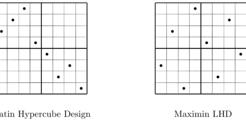
To clarify the limitations of a standard LHD, Figure 7 shows the sampling space divided into 4 subspaces. The random permutation approach could result in the situation seen to the left, not covering large pieces of the sampling space at all, although a valid LHD.
Latin Hypercube Design Maximin LHD
� � � � � � � � � � � � � � � �
Figure 7: Different LHD sampling techniques. To the left, a LHD generated by random permutation of the main diagonal. To the right, a maximin LHD where the sample points are guaranteed to spread out.
In the right picture, a maximin LHD where the minimal Euclidian distance between each pair of sample points is maximized, at the same time fulfilling the special structure of a LHD. The maximin LHDs are clearly preferable.
It is possible to use any norm when generating these designs, but most common are the 1-norm and ∞-norm besides the standard Euclidian norm (or 2-norm). A large collection of maximin LHDs and other spacefilling designs are avail-able at http://www.spacefillingdesigns.nl together with state-of-the-art articles in the area.
14
Experimental Designs Random Sampling Designs
Randomly choose a point x ∈ Ω, or optionally x ∈ ΩC to handle constraints,
and forbid points inside a circle with center x and radius r. Randomly select a new point, reject it if too close to any previous points. Repeat until n points are found. The result is not necessarily non-collapsing, as hinted by Figure 8. At a closer look, we see that the radii of points 11 and 12 do overlap some of their adjacent circles. It is simply not possible to fit the last two circles inside the box, given the randomly chosen locations of the previous 10 points.
−5 0 5 10 0 5 10 x1 x2 x3 x4 x5 x6 x7 x8 x9 x10 x11 x12 xU xL
Random Sampling Design
Figure 8: Example of a Random Sampling Design. For this 2-dimensional problem, 12 points have been sampled iteratively to fit inside the bounding box, marked with a dotted line.
The Random Sampling Design (RSD) algorithm generates the n sample points one at a time by randomly choosing a point inside the bounding box. If the circle does not overlap any other circles, the point is saved. If the circle do overlap another circle, the point is rejected and a new point is randomly generated. This is repeated until n sample points have been found.
To handle the situation seen in Figure 8, where it is not possible to fit the last two circles, the RSD algorithm use a specified finite number of points to reject. For each rejected point, a violation measure is calculated, and the least infeasible point is always saved. If the limit is reached, still without a feasible point, the least infeasible point is used instead.
This method is a good substitute for a maximin LHD, at least for sufficiently large values of r. Finding a maximin LHD is not easy in general, especially in higher dimensions, hence we recommend using a RSD instead if no suitable maximin LHD is available.
Algorithms for Costly Global Optimization Latin Hypercube Designs
Latin Hypercube Designs (LHD) is a popular choice of experimental design. The structure of LHDs ensure that the sampled points cover the sampling space in a good way. They also have a non-collapsing feature, i.e. no points ever share the same value in any dimension. It is also extremely easy to generate a
LHD. Suppose we need to find n sample points x ∈ Rd, then simply permute
the numbers 1, . . . , n, once for each dimension d.
Maximin LHDs give an even better design, as the points not only fulfill the structural properties of LHD designs, but also separate as much as possible in a given norm, e.g. the standard Euclidean norm. They are much harder to generate though, except for some special cases in 2 dimensions, using the 1-norm and ∞-norm, described in [15].
To clarify the limitations of a standard LHD, Figure 7 shows the sampling space divided into 4 subspaces. The random permutation approach could result in the situation seen to the left, not covering large pieces of the sampling space at all, although a valid LHD.
Latin Hypercube Design Maximin LHD
� � � � � � � � � � � � � � � �
Figure 7: Different LHD sampling techniques. To the left, a LHD generated by random permutation of the main diagonal. To the right, a maximin LHD where the sample points are guaranteed to spread out.
In the right picture, a maximin LHD where the minimal Euclidian distance between each pair of sample points is maximized, at the same time fulfilling the special structure of a LHD. The maximin LHDs are clearly preferable.
It is possible to use any norm when generating these designs, but most common are the 1-norm and ∞-norm besides the standard Euclidian norm (or 2-norm). A large collection of maximin LHDs and other spacefilling designs are avail-able at http://www.spacefillingdesigns.nl together with state-of-the-art articles in the area.
14
Experimental Designs Random Sampling Designs
Randomly choose a point x ∈ Ω, or optionally x ∈ ΩC to handle constraints,
and forbid points inside a circle with center x and radius r. Randomly select a new point, reject it if too close to any previous points. Repeat until n points are found. The result is not necessarily non-collapsing, as hinted by Figure 8. At a closer look, we see that the radii of points 11 and 12 do overlap some of their adjacent circles. It is simply not possible to fit the last two circles inside the box, given the randomly chosen locations of the previous 10 points.
−5 0 5 10 0 5 10 x1 x2 x3 x4 x5 x6 x7 x8 x9 x10 x11 x12 xU xL
Random Sampling Design
Figure 8: Example of a Random Sampling Design. For this 2-dimensional problem, 12 points have been sampled iteratively to fit inside the bounding box, marked with a dotted line.
The Random Sampling Design (RSD) algorithm generates the n sample points one at a time by randomly choosing a point inside the bounding box. If the circle does not overlap any other circles, the point is saved. If the circle do overlap another circle, the point is rejected and a new point is randomly generated. This is repeated until n sample points have been found.
To handle the situation seen in Figure 8, where it is not possible to fit the last two circles, the RSD algorithm use a specified finite number of points to reject. For each rejected point, a violation measure is calculated, and the least infeasible point is always saved. If the limit is reached, still without a feasible point, the least infeasible point is used instead.
This method is a good substitute for a maximin LHD, at least for sufficiently large values of r. Finding a maximin LHD is not easy in general, especially in higher dimensions, hence we recommend using a RSD instead if no suitable maximin LHD is available.