Image optimization algorithms on an FPGA

Image optimization algorithms on an FPGA

Kenneth Ericsson

School of Innovation, Design and Engineering. Mälardalen University

Robert H. Grann

School of Innovation, Design and Engineering. Mälardalen University

Supervisor: Jörgen Lidholm Examiner: Lars Asplund 2009-04-02

Abstract

In this thesis a method to compensate camera distortion is developed for an FPGA platform as part of a complete vision system. Several methods and models is presented and described to give a good introduction to the complexity of the problems that is overcome with the developed method. The solution to the core problem is shown to have a good precision on a sub-pixel level.

1 Introduction... 4

1.1 Background... 4

1.2 Purpose ... 5

1.3 Delimitations ... 5

1.4 Conventions, abbreviations and notations ... 6

2 Related work and related theory ... 7

2.1 Problem formulation... 8

3 Analysis of problem... 9

3.1 Theory of the camera... 9

3.1.1 Lens Theory ... 10

3.1.2 Thin Lens Theory... 10

3.1.3 Thick lens Theory ... 11

3.1.4 An introduction to camera modelling. ... 12

3.1.5 Camera coordinate systems... 13

3.1.6 The Pinhole Camera Model. ... 13

3.1.7 An introduction to affine transformation. ... 15

3.1.8 The new generic camera model. ... 16

3.2 Model/Method ... 16

3.2.1 Introduction to the vision system ... 16

3.2.2 The calibration toolbox ... 17

3.2.3 Correction alternatives ... 19

4 Solution ... 24

4.1 The VHDL component ... 24

4.1.1 Fixed-point numbers representation... 25

4.1.2 The LUT file maker. ... 26

5 Results... 27

6 Summary and conclusions ... 27

7 Future work... 27 Appendix 1 ... 31 Appendix 2 ... 32 Appendix 3 ... 35 Appendix 4 ... 36 Appendix 5 ... 37 Appendix 6 ... 39 Appendix 7 ... 40 Appendix 8 ... 41 Appendix 9 ... 44

1 Introduction

1.1 Background

Robot vision and machine vision are two major branches focusing towards basically the same goal, to give the machine properties that make them able to make own decisions which decrease the amount of work done by hand to automate some process. Whether the process is to recognize doors, tables or people, cogs, nails or raw-material some basic tools are needed, a sensor or device that gather information from the surrounding environment, a processing unit that translate the gathered information, software that can interpret the information and take an accurate action based on the information and finally some kind of manipulator that is fulfilling the physical action. A good description of machine vision is stated in [1], “Machine vision is concerned with the automatic interpretation of images of real scenes in order to control or monitor machines or industrial processes. The images may be visible light, but could also be of x-ray or infrared energy, and could even be derived from ultrasound information.” this shows the width of vision. Multiple different sensors could be used to derive the information needed for the specific task, as long as the information can be interpreted into something useful e.g. manipulation by grippers on industrial robots or obstacle avoidance by an autonomous robot. Today’s advanced vision systems used in industry is often built with expensive, high precision cameras. This type of camera has a low degree of distortion which mean that the camera give a good representation of reality, the so called object world. To reduce the cost of vision systems, less sophisticated cameras could be used, similar to inexpensive web cameras. The drawbacks of using these low quality cameras are that the system has to compensate for a big amount of distortion and different kinds of distortion. Compensate distortion, could be illustrated as putting glasses on a camera, to find the correct characteristics of the glasses a calibration has to be carried out. In this thesis some methods to compensate image distortion by software, that could be implemented on programmable hardware, FPGA, is presented together with a well-known calibration method [16].

Sources of distortion might be several, but the lens of a simple camera is one of the greatest sources of error, compare the radial and tangential error in Figure 1 and Figure 2 in Appendix 2, also see the plots of error in [1], the lens might incorporate a wide variety of errors e.g. the well known fish-eye lens which has very much so called radial distortion, the fish-eye lens has a very wide viewing angle and thus expose the camera sensor to a big amount of the object world, this might of course be a wanted phenomenon, but could also be a major obstacle when different post processing methods is to be used in the system. Pictures taken with this kind of lens

look like the picture in Appendix 6, as can be seen in the example straight lines look bent, this kind of distortion is inherent in all kind of lens systems, the cameras used during experiments and testing in the thesis does not have as severe distortion as with a fish-eye lens.

1.2 Purpose

At the School of Innovations, Design and Engineering at Mälardalen University, a vision system is under development, the system is built according to the picture in Appendix 1. The system is primarily used for robot navigation but is also used in other areas of vision where distance measurement is needed e.g. pick and place [11]; the triangulation [10] capability with the stereo vision system is powerful and could basically be used in any area where a cheap alternative to expensive measurement systems is preferred. The system has some major issues due to the simplicity of the cameras and built in imperfections of the camera carrier circuit board, when image data is collected it contains some degree of distortion. Several different post processing algorithms is and will be implemented on the system such as corner detection, blob detection and object recognition, the different areas of use demands good resemblance according to correct information between the right and left picture data, in the present form the system can’t reach the precision that is desired due to the distortion.

1.3 Delimitations

The calibration method that is used to extract the camera parameters is performed offline which means before the system is put in use, the parameters is then known in advance.

1.4 Conventions, abbreviations and notations

Notation Description

FPGA Field Programmable Gate Array

FPD Field Programmable Device

ASIC Application Specific Integrated Circuit

CPLD Complex Programmable Logic Device

OS Operating System

SRAM Static Random Access Memory

DLT Direct Linear Transformation

PCM Pinhole Camera Model

GCM General Camera Calibration

CMOS Complementary Metal Oxide Semiconductor

LIV Light Intensity Value

LUT Look-up Table

KK Camera parameter matrix

kc Distortion parameter matrix

f Focal Length y x CC CC , Principal Point ) , ,

(X_w Y_w Z_w World coordinate system ) , , , , ,

(Xo Yo Zo

α

o

β

o

γ

o Object coordinates and angles

) , , , , ,

(Xc Yc Zc

α

c

β

c

γ

c Camera coordinates and angles i

i Y

2 Related work and related theory

A short introduction is given to the computing hardware used in the thesis the so called Field Programmable Gate Array, FPGA; which is one type of field programmable device, FPD. Other types of programmable logic are presented in [1], where the FPGA is presented more thoroughly. The development within the area of FPDs is very fast, one improvement was the possibility to use a programming language, for example VHDL, Verilog or Handle-C. These decrease implementation time compared to traditional scheme construction. VHDL and Verilog have opened a door to more complex circuit constructions; it is possible to implement processors, operating systems, and connections between hardware and OS.

One of the great strengths of FPGAs is the possibility to build highly parallel systems, they are not as fast as conventional general processing units considering clock frequency, but the possibilities to perform a big amount of calculations every clock cycle make the FPGA a good replacement for micro controllers which are the most used technology in embedded and small real-time systems. The procedure, from code to a working program on FPGA is as follows, programs are created in a suitable tool, the code is then synthesized which is similar/equal to compilation, the next step is to connect in- and output pins of the FPGA to the external devices, final step is to load the synthesized code into the FPGA. A deeper description of how the code looks like and how programs are built is found in [4]. FPGAs are mostly used in products that are produced in small series and in prototype constructions. If big series are to be made the VHDL/Verilog construction can be statically put into an Application Specific Integrated Circuit, ASIC. The difference in market price is still large between FPGAs compared to ASICs, which is why large series are made in ASICs although they are impossible to reprogram. The difference in price is slowly decreasing, resulting in the possibility to more often use FPGAs in larger consumer product series but as stated still uncommon. FPGA systems are found in many different areas of technology, e.g. airplanes, robotics, military equipment, cars, hand held media devices, set-top boxes and cell phones.

Camera models, calibration and correction methods have been well studied in research, [5][6], [8], [16], and several introductions to the methods can be found through internet. Only a handful has a similar concentration as our thesis present, the following papers cover similar work, [12], [13], [14], [21], [23]. David Eadie et. al. [14] present several approaches to pixel correction; they investigate the possibility to use Field Programmable Gate Arrays to enhance the calculation speed of the commonly known heavy calculations needed to correct images. Further more they examine whether it is suitable to use fixed point, floating-point and logarithmic number representation for their image processing algorithms, performance results are presented in terms of execution time and resource requirements. The results look promising, see Table 1 and strengthen the theory that FPGAs is well suited for this type of image processing, pipelining is as they state the key to extra high performance, and this can easily be seen in the results. The conclusion of the work is pointing towards one common denominator; FPGAs can reach speeds that are multiple magnitudes greater than possible with general processing units. As seen in Table 1 the difference in results is quite astonishing, the lookup table implementation is preferred when resources is to be used for further calculations, one of the few major issues with the methods is the fact that they use a big amount of SRAM.

Implementation Area (%) SRAM (MB) Clock speed Time (ms) 600x600 pixels

Pentium 4 real time calculation n/a n/a 1.7 GHz 780

Pentium 4 lookup table n/a n/a 1.7 GHz 760

Non-pipelined FPGA real time

calculation 63 5 10 MHz 360

Non-pipelined FPGA lookup table 7 7 22 MHz 130

Pipelined FPGA real time calculation 64 5 25 MHz 15

Pipelined FPGA lookup table 6 6 34 MHz 11

Table 1: Content taken from David Eadie et. al. [14], the FPGA implementations clearly have an advantage over the GPU in all aspects.

Álvaro Hernández et. al. [13] proposes an architecture that is implemented in FPGA. The architecture has some core features from [14] and has a similar working flow as in [15], but the work present a closer to solution architecture that is well suited for an FPGA. The only concern is that the paper does not present an estimation of resource requirements, nor performance figures, the proposed implementation could on the other hand be implemented for evaluation thanks to the well-described architecture. The conclusion of the authors work is that this kind of architecture could play a great role in low cost, high-resolution photography, especially as the architecture is able to handle dynamic zoom and focus with an extension.

Janne Heikkilä and Olli Silvén [16], present a four-step calibration method. They give a good view of how to derive parameters and pinpoint which parameters are needed for a correct calibration, both extrinsic and intrinsic. They conclude that direct linear transformation, DLT, and similar direct methods are computationally fast but have a couple of disadvantages, distortion cannot be added to the calculation and therefore not calculated in most cases, still a couple of solutions to this problem have been proposed as extensions to the DLT, another issue is the accuracy which according to Heikkilä and Silvén is below acceptable levels, the accuracy problem come from the presence of noise which is always a component when dealing with measurements. The paper suggest a combination of DLT and nonlinear methods to calculate parameters, the DLT is used to get good initial values that is used as starting point for an iterative method, in this work the Levenberg-Marquardt optimization method is used, the DLT estimation decrease the risk of ending in a local minimum which would destroy the calibration. The experimental part is concentrated on correcting images, not on calibration that the writers show in a prior work [5], the result show that the error is below pixel level, sub pixel precision, in realistic conditions errors below 0,01 pixels is expected according to results in their prior work.

2.1 Problem formulation

The objective of this thesis is to get familiar with some of the common calibration techniques and methods used in vision- and camera systems of today, differences and suitability is compared, a method or several methods to compensate distortion will be developed and implemented in programmable hardware, FPGA, focusing on throughput and footprint. Results from the master thesis will be added to the research group at the School of Innovations, Design and Engineering at Mälardalen University, the vision system developed in the research group has no correction for camera distortion which results in problems to map the 2D images to 3D models. Another problem will also occur, if a point in a stereo/multi camera system is detected

and matched as the same point it will start to differ when it comes closer to the edges of the picture, see figure 3 in Appendix 1.

The goals of the master thesis were to:

• Get a general understanding of camera calibration • Present several camera models and their differences • Develop correction methods for FPGA

• Implement a suitable method

Calibration and compensation has been well covered by research, but few have worked with speed and footprint in mind, thus hard to use in inexpensive and relatively slow hardware. This is one of the greatest challenges of this project, to develop a correction method suitable for the hardware in hand, as any one can imagine it is a great task to be able to use a similar working flow of [15] or at least have a result similar or better than that program, especially as the hardware used in the thesis is about 20 times slower with regard to clock speed, than a common personal computer, on top of this the system is supposed to do different post processing of the picture data e.g. corner detection [17], spin-image [11].

3 Analysis of problem

3.1 Theory of the camera

This text is a short description of how a camera works, more complete information can be found in for example “Computer Vision -- A modern approach” [18]. The simplest camera is the pinhole camera (camera obscura), Figure 1. The pin-hole camera was first described in documents from Mozi (470 BC to 390 BC), a Chinese philosopher. The first realized version is known from the sixteenth century and uses a small hole instead of a lens. Light reflected from an object in this case a candle goes through a pinhole and projects on the image plane. Observe that the image appears upside down on the image sensor. In theory only one light ray from every point of the object passes through the pin hole. Today it is more common that a camera uses a positive lens instead of a simple pin hole. To use a lens in a camera gives advantages in form of higher resolution and higher sensitivity but also problems as short focus depth due to a large aperture. Most common lenses have anomalies that cause distortion. It is hard to manufacture a good lens and that’s why a good lens often is rather expensive. A good lens is often a combination of several lenses with different properties mounted into one unit.

Figure 1: The camera obscura.

There are several different kinds of distortion that can occur in this report we will show two of the most common distortions radial and tangential see Figure 2.

Figure 2: The figure to the left shows a normal not distorted image, the figure in the middle shows an image with pincushion distortion and the image to the right barrel distortion.

3.1.1 Lens Theory

To understand optics we will use a simplified model of how a lens works. The thin lens model is simplified in that way that you can see the lens as a layer that are able to deflect the rays only one time and only in the middle of the lens, could be seen as an atomic membrane. The opposite is the thick lens that deflects the rays two times both on the way into the lens body and on the way out of it. The thick lens model is more complex and has many parameters. One parameter is the aperture or light intake width. The aperture controls the focus zone, more about this later.

3.1.2 Thin Lens Theory

Figure 3: Light rays way through a thin lens.

In a system with a thin lens, diverted rays from an objected will focus on the image plane, Figure 3. The light rays’ way through the lens is depending on the angle of approach. Light rays from the object that are parallel to the optical axis will deflect through the focal point on the image plane side of the lens. Light rays that intersect the optical axis in the middle of the lens will not be deflected. Light rays that intersect the optical axis on distance f in front of the lens will go in parallel with the optical axis after the ray has been deflected through the lens, see Figure 3. In this figure the aperture is big which means that a lot of light rays from the same object point end up onto the image plane; this will result in increased resolution but gives, on the other hand, a shorter focal length.

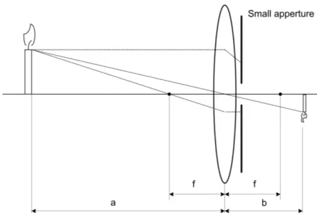
Figure 4: Light rays way through a thin lens with small aperture.

If the aperture is small the camera behaviour will be like a pin-hole camera, this is because rays that have their intersection of the optical axis different from the middle of the lens will be hindered by the small aperture, see Figure 4. The good thing with small aperture is an increased focal depth; the drawback is lower resolution and lower light sensitivity.

Figure 5: Parallel rays.

Light rays parallel to the optical axis will be deflected into the focal point, Figure 5. This means

that ,. + = ⇒ f b a 1 1 1 f b a→∞⇒ ≈ see Figure 4.

3.1.3 Thick lens Theory

Thin lenses is only a simplified theoretical model and have very little to do with real lenses. Even though the model is simple it can be a seed to a complex camera model. Real lenses are more complicated and therefore they have a special model called thick lens model.

Figure 6: Light rays way through a thick lens.

The thick lens model is more complicated to define. Only light rays that travels on the optical axis, the dashed line, remains undeflected see Figure 6. That means that the focal point is harder to find and the focal point cannot be seen as a single point, rather like a floating focal zone, see Figure 7. Here we instead can talk about a point of less confusion. The Point P in Figure 7 will appear as a circle due to the picture plane position, the point of so called less confusion is found at the dashed line, this is where the most information co-occur, another phenomenon that is modelled is the so called vignetting. If a more concentrated point is expected you can use several lenses in a lens system with unique characteristics. The drawback of the thick lens is that some of the light rays that end up on the edge or corner of the lens will not pass the lens system correctly, the rays that pass the lens will end up beside the image sensor, and this effect is the vignetting, see Picture 2 in Appendix 6.

Figure 7: Point of less confusion at the dashed line.

3.1.4 An introduction to camera modelling.

A camera model is the connection/interface between the real world that is represented in 3D and the image represented in 2D that will be reproduced on the image sensor. A camera model is a mathematical model of the characteristic associated with a camera. Included in the camera

model is the lens and sensors characteristic i.e. distortion that comes from inconsistency built in, both in the lens and the sensor. The distortion can also come from misplacement of both lens and sensor. A camera model can be simple or it can be complicated but one common thing is both can predict the light rays’ way from the object into the image sensor and the other way around. Some differences between a simple and a more complex model can inter alia be that the more complicated model manages zoom, focus and wide angle lenses like fish-eye lenses a lot better. Notable is that you lose one degree of freedom when you go from 3D into 2D which means that it is impossible to go back to 3D again from only one image. If the goal is to get the 3D information you need two cameras imaging the same thing from two directions.

Camera models contain a number of different parameters called intrinsic and extrinsic, the intrinsic parameters describe the light rays’ way through the lens onto the image sensor, whilst the extrinsic parameters describe the camera position and heading in the world coordinate system. The intrinsic camera parameters are different between different camera models while the extrinsic parameters often are the same.

3.1.5 Camera coordinate systems.

When a camera model is to be defined the first things that have to be done is to define all the involved coordinate systems, Figure 8. We need to define one global coordinate system to represent the world,(X_w,Y_w,Z_w) another coordinate system including its rotations is needed for each object,(X_o,Y_o,Z_o,

α

_o,

β

_o,

γ

_o), the camera coordinate system and the angles of rotation in each axis, the so called heading, is defined as (X_c,Y_c,Z_c,

α

_c,

β

_c,

γ

_c), see Figure 8. The last two definitions are known as the extrinsic camera parameters and is seen in Figure 8 as the external coordinate system of the camera; inside the camera there is another coordinate system, the image coordinate system that is a 2D coordinate system and a part of the camera model and the so called intrinsic camera parameters.

Figure 8: Several coordinate systems involved.

3.1.6 The Pinhole Camera Model.

The most uncomplicated camera model is the Pinhole Camera Model, PCM. The PCM is a model of the first camera built out of a box and a little hole as a thin lens. The principal of a Pinhole Camera is shown in Figure 9. The light rays way from the object to the optical sensor can be seen as a straight line from the object through the pinhole onto the image sensor, see Figure 9. The Pinhole camera technique is modelled as two linear equations one for X and one

for Y. Included in the linear equations (0.1) and (0.2) is the focal length fx,y as a scale factor

and the principal point CC_x,y as an offset.

x x o i X f CC X = ⋅ + (0.1) y y o i Y f CC Y = ⋅ + (0.2)

This mapping between the object space and the image space is also called affine transformation; affine transformation will be described later in this report. Often matrices are used for this kind of calculation, with an affine transformation matrix multiplication it is possible to both do the scaling, rotation, translation and skew in one matrix calculation. X ,_i Y_i is the normalized position on the image plane. X ,_o Y_o is the position on the image sensor in pixels. The equations are used to project the light rays from the object onto the image sensor, the camera model can then be added with more feature parameters as for example radial and tangential distortion. In the Matlab toolbox later used in this work polynomial equation of fourth order is used to model radial distortion, the model also include extrinsic parameters.

3.1.7 An introduction to affine transformation.

Affine transformation is when a set of points formed as a figure or as in this case an image is manipulated so its form can be restored. Both 2D and 3D objects can be manipulated as for example a cube that can be scaled, rotated, moved and skewed and then restored to its original looks. As a calculation example the 3D point in Figure 10 is used to demonstrate how and what could be done with the help of affine transformation. A good approach is to use matrices when calculating affine transformations.

Figure 10: A 3D object point is mapped onto the image plane.

Let P be a 3D object point as a 1 by 4 matrix and T, translation matrix, is the movement in each directions as a 1 by 4 matrix. P´ is the result from this matrix addition in form of a 1 by 4 matrix, see (1.1).

T P

P′= + (1.1)

In this example P is the same 3D object point as a matrix 1 by 4 and R is the scaling, rotation and/or skew in each direction as a 4 by 4 matrix. P´ is the result from this matrix multiplication in form of a 1 by 4 matrix, see (1.2).

P R

P´= ⋅ (1.2)

It is possible to perform several transformations in one matrix calculation according to (1.3).

            •             =             ′ ′ ′ 1 1 0 0 0 6 5 4 3 2 1 1 z y x z y x z y x P P P T s s T s s T s s P P P

λ

κ

δ

(1.3)

The scaling, skew and rotation is applied on the 3 by 3 positions in the upper left-hand corner of the 4 by 4 transformation matrix, the translation is applied on the T ,_x T_y and

T

_z parameters. Below is a description of the different transformation parameters that could be applied.

δ

Scaling in X

κ

Scaling in Y

λ

Scaling in Z 1 s X skew in respect to Y 2 s X skew in respect to Z 3 s Y skew in respect to X 4 s Y skew in respect to Z 5 s Z skew in respect to X 6 s Z skew in respect to Y





















−

θ

θ

θ

θ

cos

sin

0

sin

cos

0

0

0

1

Matrix for rotation about the x axis





















−

θ

θ

θ

θ

cos

0

sin

0

1

0

sin

0

cos

Matrix for rotation about the y axis





















−

1

0

0

0

cos

sin

0

sin

cos

θ

θ

θ

θ

Matrix for rotation about the z axis

The affine transformation is in our work used to transform a point in the object world to a point on the image plane.

3.1.8 The new generic camera model.

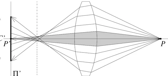
The Generic Camera Model, GCM, is an approach to do a camera model that can model properties like focus, zoom, big aperture and wide angle lenses. The concept of the model is seen in Figure 11. Anders Ryberg is this models inventor, more information about the GCM can be found in [19].

Figure 11: The General Camera Model, GCM.

3.2 Model/Method

The vision system that has been used during testing is presented below; in the rest of the chapter the methods and tools will be presented.

3.2.1 Introduction to the vision system

Base of the vision system is the FPGA motherboard; the board includes, inter alia, a Xilinx Virtex-II XC2V8000 eight million gate equivalents FPGA, for further specifications see [22], 512MiB 133MHz mobile-SDRAM memory and USB connectivity via an external FTDI FT245R chip. The cameras, up to four, is connected via a parallel interface, the camera carrier boards include the CMOS sensor and mounting holes for different lense holders, Appendix 1 and Appendix 4. The sensor chip, MT9P031, manufactured by Micron

frame rate that can be achieved with the sensor is 123 fps in VGA (640x480) mode, maximum rate at full resolution, (2592x1944), is 14 fps. In Figure 12 the block diagram of the sensor is shown.

Figure 12: Block Diagram of Micron MT9P031 CMOS sensor.

The different signals represented in the figure as arrows pointing in to and out from the sensor boundary is used to communicate, set up and read the sensor. Most of the signals are physically connected to the FPGA board through I/O pins; the specific meaning of the different signals is presented in the data sheet of the sensor, most interesting is the Dout[11:0] signal that carry the pixel light intensity data. A picture of the complete system mounted for testing are found in Appendix 1.

3.2.2 The calibration toolbox

There are several methods of correction that will be presented with their benefits and drawbacks, and if the method is suitable for a certain hardware or area of use this will be presented as well. All the methods that is presented have a pre-calculation stage made off line, there for before a correction of a picture can be done it is necessary that the camera model parameters is known. There are several methods to obtain those parameters, in this thesis the Matlab toolbox from [15] is used for collecting data from pictures of a checker pattern plane. The toolbox is very useful and produces the camera parameters wanted and estimates the calculation errors. The input to the toolbox is a set of pictures from different angles see Figure 13; the output is the camera parameters presented as seen below in Table 2. The data can then be used to correct the pictures used to obtain the parameters or all other pictures taken with the same camera. The toolbox is built on methods presented in Zhengyou Zhang “Flexible Camera Calibration By Viewing a Plane From Unknown Orientations”, [20], and Janne Heikkilä and Olli Silvén’s paper “A Four-step Camera Calibration Procedure with Implicit Image Correction.”, [16].

Table 2: Example of camera parameters.

Focal Length, fc, pixels [511.82267, 506.45123] ± [11.28509, 12.19115] Principal point, cc, pixels [323.15503, 208.70276] ± [13.28817, 12.38071] Distortion, kc [-0.40015, 0.16697, -0.00155, 0.00010, 0.00000] Uncertainties ± [0.03214, 0.06170, 0.00529, 0.00366, 0.00000] Pixel error, err [0.71862, 0.28875]

EXTCLK RESET# STANDBY# OE# Pixel Array 2,752H x 2004V A rr ay C o n tr o l Serial Interface O u tp u t

Analog Signal Chain Data Path

SCLK SDATA SADDR PIXCLK DOUT[11:0] LINE_VALID FRAME_VALID STROBE TRIGGER

Figure 13: 20 pictures taken from different angles to cover as many positions as possible.

A short summary of how the toolbox works:

The algorithm needs a couple of thousand point-couples to calculate a good camera model. A point-couple is two points, one on the sensor plane and one on the object plane. To get one point-couple you have to make a connection between the two, the Matlab toolbox can manage to make those point-couples with help from the user. You have to load a set of calibration images into Matlab where the user needs to point out the corners, Figure 14, of the checker calibration pattern for each picture. It is important that the pictures have as many different angles as possible to make the camera model prediction better and more correct. After the corners are selected the toolbox tries to find every corner between the selected corners. The user has to control that everything is correct; when everything is fine the user starts the calibration, which is automatic.

Figure 14: An example picture of how to pinpoint the corners of the checker test pattern.

Click #4

Click #3

Click #2

Click #1 (Origin)

3.2.3 Correction alternatives

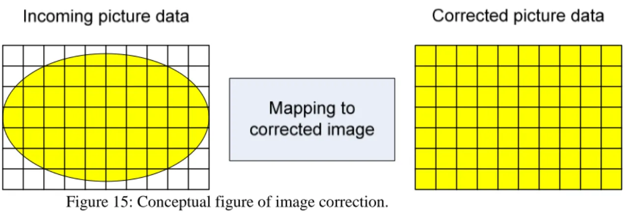
In Figure 15 the basic concept of image correction can be seen, this figure will be referenced to describe the distinctive features of the different methods of correction, amount of error and type of error due to the method will be presented as well.

Figure 15: Conceptual figure of image correction.

Online correction calculation

The camera and distortion parameters known in advance is used to do calculations on the incoming picture data, a similar process as with the Matlab toolbox is performed, some of the major issues with this method is that a big input buffer and a big output buffer is needed due to the bilinear interpolation of pixels and the serial data. The ellipse in Figure 15 represents the data that should be fitted to the whole outgoing correct image, as one can imagine the data in the incoming frame is not sufficient to fill the outgoing frame as the data is stretched out, with a interpolation technique, on more pixels then the amount that is moved i.e. the amount of moved pixels are less then the outgoing frame

n

×

m

pixels. Correction of an image is performed as follows, x_in and y_in coordinates of the outgoing frame is used to calculate which pixel data, light intensity, from the distorted picture that should be moved to the x_in and y_in coordinate. The first calculation that needs to be done is the affine transformation from correct pixel coordinate x ,_in y_in to the coordinate that the pixel data should be derived from. Matrix KK is the so called camera matrix, parameters in this matrix is derived from the Matlab toolbox, precise descriptions of the parameters is found in [9].





















=

1

0

0

)

2

(

)

2

(

0

)

1

(

)

1

(

)

1

(

cc

fc

cc

fc

fc

KK

c

α

The inverse camera model is applied to add the inverse mapping, (2.1), between the theoretically correct pixels in the outgoing correct frame, and the incoming distorted frame:













=













⋅

− 1 1 1

y

x

y

x

KK

in in (2.1) 2 1 2 3 2 1 2 2 1 1 1 2 1 2 1 2 2 2 2 y r a x r a y x a y x r + = + = ⋅ = ⋅ =

The implicit inverse model include radial and tangential distortion accoring to the following calculations.

2 1 4 2

)

4

(

)

3

(

)

2

(

)

1

(

1

a

kc

a

kc

tad

r

kc

r

kc

rad

x

+

=

+

=

+

+

=

(2.2)

The last affine transformation into pixel coordinates, (2.3), include the distortions, the xout and yout

coordinates are representing the coordinates where the data of the correct pixel is to be derived from.





















=





















+

+

⋅

1

1

1 1 out out y x

y

x

tad

rad

y

tad

rad

x

KK

(2.3)

The last step before correction is to perform bilinear interpolation [8]; the reason is to fill the missing information due to the stretching and fitting of the correction procedure mentioned before. To begin with the

out

x and yout values is rounded off to get the coordinates of pixel A, see figure below. Pixel A, B, C and D

consist of a position and a light intensity value i.e. the numerical representation of the light intensity.

) ( ) ( )) ( 1 ( ) ( ) ( )) ( 1 ( )) ( 1 ( )) ( 1 ( , A out A out D A out A out C A out A out B A out A out A Yin Xin x x y y LIV x x y y LIV x x y y LIV x x y y LIV LIV − ⋅ − ⋅ + − − ⋅ − ⋅ + + − ⋅ − − ⋅ + − − ⋅ − − ⋅ =

The weighted Light Intensity Value, LIV, of the pixels surrounding xout and yout will be moved to position in

in y

x , in the outgoing image, this procedure need to be done to each pixel. As can be seen in the bilinear interpolation calculation, [7], four pixels around the pixel under inspection (xout,yout) are needed to move the weighted data to the corrected positionx ,in yin. Another important notice is the fact that the incoming

picture data is serial and read from the upper left corner, thus the data until the first pixel that should be moved in a row is discarded. This method needed a big input buffer the reason is the awkward process that begin with the theoretically correct coordinate (1, 1), the data used for that pixel is read several rows later than the row of the first pixel that actually could be moved; an example is shown in Figure 16 below. To keep the order of the pixels intact the system needs to store several pixels in the buffer. In the example figure it seems like a small problem, but in a real world situation the distortion could be way worse, thus the difference produces a need of a big input buffer. To estimate input and output buffer some pre-calculations need to be done, maximum and minimum y value of the first and last outgoing rows need to be calculated. The maximum value of

∆

Y

₁ and

∆

Y

₂ described in Figure 16 and Figure 17 below is used to describe the calculation of the buffer size.

out x out y A B C D

β

1 1

Figure 16: Concept and example of how pixels are moved.

Figure 17: Concept and example of how output buffer could be calculated.

The good points of the online correction calculation method is the precision which keep a sub pixel level of approximately 0.01 pixels [16], another good thing is that even though it requires a large amount of memory, it consume less memory than the simple lookup table method, see [13], problems of the procedure is the relatively huge amount of FPGA resources needed, several multipliers is needed and the amount will increase with the amount of parallelism.

Lookup table, Basic technique

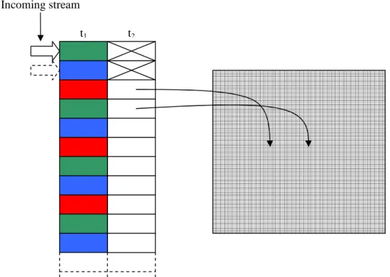
The second method that is analyzed and further developed is the idea of using lookup tables to perform direct correction of the incoming pixels. As previously mentioned in the related work the lookup table technique has already been exploited but only simulated without real life constraints such as limited amounts of memory. Several versions have been developed based on the most simple lookup table technique; the concept of the technique is shown below, Figure 18. The same pre-calculations as in the prior method have to be carried out to make it possible to calculate which pixels should be mapped and moved into the correct image. When all parameters is known every pixel in the correct image is pre-processed through the affine transformations and calculations

As mentioned earlier the most basic look-up technique is to map the incoming serial stream of pixels to a certain movement into the new, correct, image. A couple of drawbacks are the bad scalability; if the resolution is changed the whole map has to be re-calculated, the second drawback is the amount of memory that easily can exceed 2MByte when high resolutions is used, the amount of reading from memory will also slow the system down as the readout will intrude on other post-calculation algorithms that utilize the same memory. With this in mind some other techniques had to be developed to minimize the memory usage.

Figure 18: Basic concept of how the simple look-up table technique work, table t1 show the incoming pixel data, t2 include the correction of the incoming pixel, the crossed boxes show an example of pixels that shouldn’t be moved.

Compressed tables

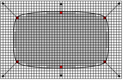
A good alternative to the simple table is to apply a compression algorithm on the table. As can be seen in Fel!

Hittar inte referenskälla.Figure 16 and Figure 17 the only data that should be moved to the corrected image

is the colored area, the other incoming pixels are as an example marked with cross in Figure 18, pixels that should not be moved. Big parts of the table will include the crossed pixels and can thus be chunked together to just one start and stop pixel decreasing the amount of needed memory considerably, the same procedure applies to the whole table. Gain in decreased memory usage is directly related to the amount of distortion, the more distortion the higher the memory reduction will be. One of the other big benefits of the compressed table is decreased amount of reading, it’s easily understood that by just reading two consecutive rows of pixels a lot of pixels could be moved or dispatched. Several other compression algorithms could probably be used but will not be covered in this work.

Support tables

Another possibility is to use look-up tables containing pre-calculated parts of the calculations in the online correction calculation chapter, 3. This is one way of decreasing the resource need of the correction algorithm. The idea of the table and how to access parts of the table is shown in Figure 19. The index is based on the squared radius of the incoming pixel, the pixel that should be moved; this calculation is easily performed with only two multiplicationsx_in2 + y_in2.

Figure 19: Lookup table r with r2 as index, used instead of the square root function.

In Figure 20 another table is shown with the correcting movement, ∆r, of a pixel with its given radius, the radius could either be calculated internally in the FPGA or extracted out of a table similar to Figure 19. As origin, incoming pixel coordinates x and y and the movement ∆r is known it is possible to calculate the new correct coordinates according to Figure 21.

Incoming stream

t1 t2

r2 - index

Figure 20: Lookup table with r as index.

Figure 21: Pixel moved with the data from a lookup table.

The radial correction∆r is calculated with an iterative process, this is called forward mapping [16], the opposite to the backward mapping used in the Matlab toolbox. To build up the table with ∆r the following process is performed; also see the pseudo code below. Calculate with the iterative method the new, correct position of the pixels; subtract the radius of the original pixel from the new radius to get all of the correction radiuses matched to original radius according to Figure 20.

FOR All pixels

X = Xin_n * Scale_factor Y = Yin_n * Scale_factor FOR n_Times r_2 = X^2+Y^2 k_radial = 1 + k1 * r_2 + k2 * r_2^2 X = Xin_n/k_radial Y = Yin_n/k_radial END X_store(n) = X * Scale_factor Y_store(n) = Y * Scale_factor END

The iterative method is the only way of directly solving the movement of distorted pixels to new corrected positions, else way the Matlab toolbox backward mapping have to be done to calculate the new positions. The major advantage of the iterative method is that the close to exact position is given in a decimal format, as an example see Figure 22 where the crosses mark the discrete position and the circles mark the real pixel positions. The non discrete positions could in post processing stages be used as is to gain better precision compared to interpolated, discrete positions, or the non discrete pixels could be interpolated into discrete positions to get visible pictures out of the system. The major drawback and the reason to why the iterative

r- index ∆r1 ∆r2 ∆r3 ∆r4 ∆r5 ∆rn y

x

r

α

α

∆r ∆y ∆x

When ∆r and r is known it is possible to move the light intensity data according to (3.1), the new x and y position of the pixel or feature:

r r y y Y r r x x X new new ∆ ⋅ + = ∆ ⋅ + = (3.1)

Figure 22: Example of corrected pixels.

4 Solution

The method that is chosen for testing and validation is based on the last method described in the Model/Method chapter, 3, what we call support tables. The reason to why this method is chosen is the combination of high precision, relatively low memory usage and decreased resource requirements compared to the online calculation correction method, [13]. Compared to the other LUT methods the chosen method utilizes less memory and due to the fact that no interpolation to pixels will be done as the correction of position only will be applied to features the precision is kept high. In our solution the new position of the features will be represented with fixed-point values instead of integer pixels. Our solution uses the Calib Toolbox [15] that supplies several parameters that describe the amount of distortion radial and tangential plus the principal point. In this solution only the radial distortion will be compensating for. The tangential distortion is harder to compensate for because it is depending on X and Y separated. A solution for compensating tangential distortion is more complex than the compensating for radial distortion. The amount of tangential distortion is within the range of 0.01 to 0.1 pixels in our example. See Appendix 2 figure 1. The tangential distortion is equal to the pixel error that can be seen in the result from the correction algorithm chosen, therefore it is not motivated to compensate for the tangential distortion.

4.1 The VHDL component

The component is rather simple; the correcting method is described later in this chapter. The components in data is pixel data of the feature position and a signal called “new_corner” tells the component when the pixel data is valid. Reset and the serial clock are also needed. Out from the component comes the new corrected feature position in fixed-point representation and a signal telling when the result is valid. A correction sequence starts with the new_corner flag and the X and Y coordinates supplied to the component. At that moment a counter starts and when the calculation is done the results comes out as new X and Y coordinates and the signal new_coordinat will be active.

New_corner X_coordinate Y_coordinate

sclk

new_X_coordinate new_Y_coordinate

reset

new_coordinate

LUT

Index Data

Feature

Correction

Figure 23: Description of the VHDL component

4.1.1 Fixed-point numbers representation

If fractional values is needed it is preferred to use fixed point representation in FPGA. Compared to floating point representation fixed point is faster and easier to use. If floating point is used some kind of hardware support is preferred. In our case the extra amount of resources a Floating Point Unit, FPU, would consume in an FPGA cannot be motivated, the reason is shown in the results chapter, 5. In fixed-point representation the number is divided in two parts, integer part and fraction part. The name fixed-point means that the size of each part is fixed and must be chosen carefully according to the range and the resolution needed. The example showed here uses 8 bits for the integer part plus 1 bit for sign and 7 bits for the fraction part. The resolution in this example is 0.0078125

128 1 ₌

. The highest value possible to represent is 255.9921875 and lowest -256.0000000. Fixed-point numbers can use all ordinary arithmetic functions such as +, -, /, * similar to ordinary integers, without restrictions.

0 1 2 3 4 5 6 7 8 9 10 11 12 13 14 15 128 1 64 1 32 1 16 1 8 1 4 1 2 1 1 2 4 8 16 32 64 128 b b b b b b b b b b b b b b b b • − +

The final solution is described below; the reason to why a deeper description is introduced is because some important differences compared to the methods in chapter 3 were done during the testing and implementation phase.

The values stored in the table for each position is

r r

∆

scaled up with 8192, because the initial value for

r r

∆

is within the range of 0.0002 to 0.1 and it is more practical to use integers in the table, to solve this in the FPGA later on the fixed-point method will be used. One of the major reasons to why

r r

∆

is stored instead of only ∆r is to save space and decrease the amount of read cycles in the lookup table. The table content now is between 2 and 809; the drawback is that the result needs to be scaled down after calculation with the same scale factor i.e. 8192, that means an extra down shift is needed, in this case 13 steps.

116500 ) 200 20 ( ) 300 10 ( − 2 + − 2 = =

I this means that if the point is near the edge, r2 is a large number

and that will demand a very big lookup-table. The solution is to scale r2with some factor; our solution is to divide 116500 with 512, which give 227 after the fraction part is cut. With this method a table for an ordinary 640 x 480 picture will end up in around 340 values. The draw back here is that in the end of the table there will be some positions containing zero, starting from the middle of the LUT and increases towards the end, the reason is the quadratic index, this problem is solved with an interpolation between the value before and the value after the current empty “zero position”, see (4.1).

2 1 1 + − + = n n n S S S (4.1)

The reason to why this interpolation gives a satisfying result is because the function represented in the LUT is close to linear.

4.1.2 The LUT file maker.

The lookup table used for the undistortion module in the FPGA can be produced directly out from Matlab by running our script-file Lookup.m. The output file is a vhd source file and can be included directly into the FPGA programming tool. It is possible to set some parameters in the script, from where the input data will come from Matlabs workspace or directly from the script file. There are also possibilities to edit the two scale factors, indexscalefactor and lookupscalefactor, the indexscalefactor is used to scale the indexing number and the lookupscalefactor is used to scale the stored values in the lookup table.

To begin with the LUT technique was implemented in Matlab, pictures with the calibration pattern is extracted from the vision system for camera parameter estimation; see Figure 1, 2, 3 and 4 in Appendix 5. With the help of the calibration toolbox [15], intrinsic and extrinsic parameters are given after the calibration, the resulting values are used in the LUT generation procedure, see Figure 24.

Figure 24: Flowchart showing the concept of correction table creation.

After the LUT is generated the data is easily accessed according to Figure 25, Fout_x,_y is the new feature position in x and y, in this stage the coordinates are represented with fixed-point notation.

Iterative pixel coordinate calculation, r_new r r r Y X r new n n − = ∆ + = 2 2

Produce the lookup table

r r 8192*

∆

Normalized coordinates Along the largest radius:X ,n Yn

Index, 512 2 2 n n Y X I = + +1 r r 8192* ∆ r r 8192* ∆ r r 8192* ∆

Figure 25: Flowchart showing the concept of pixel movement.

5 Results

The distance between the pixels moved by the iterative method and pixels moved by our lookup table method is shown in the three histograms in Appendix 7. The test results are derived from a random set of distorted pixels distributed over a 640 by 480 pixel surface according to Figure 1, in Appendix 8, it is easiest to see the movement of pixels far away from the center of the figure because the distortion is larger there, the stars in the figure symbolize the data that is derived from the sensor i.e. distorted pixels, the crosses and dark circles represent the position of the moved data, this is shown in detail in Figure 2, in Appendix 8. Due to the small distance difference between the movement methods used, an even more detailed figure has to be shown, Figure 3 in Appendix 8. The last figure show a high detail view of one moved feature, the ‘dot’ is where the feature is moved to when the LUT is used, the ‘cross’ show where the data is moved according to the Calib toolbox [15] and the ‘circle’ represent the feature moved directly by the iterative method. As can be seen the ‘dot’ doesn’t coincide with the ‘circle’, this has its reasons in several parameters such as truncation to the lookup table and interpolation in the lookup table. Looking at the histograms in Appendix 7 showing the delta distance, it is now easy to see and understand how big the impact of the scaling of the LUT index are. All figures in Appendix 7 and Appendix 8 are based on the assumption that we are able to handle real numbers, which in the FPGA will consume a lot of resources, so the solution was as earlier described to use the fixed-point method. It is possible to measure a difference in precision due to the fixed fixed-point method, comparing the second histogram in Appendix 7, Figure 2, with the histograms in Appendix 9 give a good view of the impact that the scaling of the data in the LUT has on the final precision. When the LUT data is scaled by 2048 and 4096 a significant degradation of precision is recognized, it is only when the fixed-point scale is equal or greater than 8192 that the precision approach the real number representation shown in Figure 2, Appendix 7.

6 Summary and conclusions

In this thesis a method to compensate camera distortion is developed for an FPGA platform as part of a complete vision system. Several methods and models is presented and described to give a good introduction to the complexity of the problems that is overcome with the developed method. The solution is shown to have a good precision on a sub-pixel level. A script file to extend the Calib Toolbox has been developed for auto generating the LUT as a vhd source file.

7 Future work

• What needs to be further investigated is whether the solution increases the precision of the complete system or not.

(

xy

)

xy y x Fnorm LUT I F Fout _, = _, * ( )/8192 + _, r r 8192* ∆ Feature coordinates y x F_, Index,

512

2 2 y x

Fnorm

Fnorm

I

=

+

+1 r r 8192* ∆ r r 8192* ∆ y x y x y x

F

CC

Fnorm

_,

=

_,

−

_, r r 8192* ∆ r r 8192* ∆ = ) (I LUT

• Testing with different lenses and different kind of cameras can also be a future task. Some of the improvements that could be looked into are to use an advanced interpolation to fill the zero value positions in the LUT generation procedure; another part that possibly could improve precision is to interpolate the extracted data from the LUT i.e. if the calculated index of a pixel isn’t discrete, then an interpolation of the data in the closest positions could be done.

• Also the tangential distortion can be compensated for in some future version.

• In [21] Niklas Pettersson and Lars Pettersson research the possibility to automatically extract features with hardware, they conclude that with the SIFT algorithm used it's possible to extract features for calibration with good results. This technique or a similar method could possibly be used as a base for a totally automated camera calibration procedure that could be performed during the start-up phase of the stereo vision system.

[1] Duane C. Brown, “Close-Range Camera Calibration”, Photogrammetric Engineering, DBA Systems, Melbourne, Australia, 1971.

[2] “Machine Vision Handbook”, 2009-01-03,

http://emva.org/files/machinevisionknowledge/MVHandbookLR07.pdf

[3] Stephen Brown, Jonathan Rose, “Architecture of FPGAs and CPLDs: A Tutorial”, Department of Electrical and Computer Engineering, University of Toronto. IEEE Design and Test of Computers, vol. 13, no. 2, 1996.

[4] Stefan Sjöholm, L. Lindh, “VHDL för konstruktion”, Studentlitteratur, 2003, fjärde upplagan, ISBN: 91-44-02471-1.

[5] Janne Heikkilä, Olli Silvén, “Calibration procedure for short focal length off-the-shelf CCD cameras”, Proc. 13th International Conference on Pattern Recognition, 1996. Vienna, Austria, p. 166-170.

[6] Roger Y. Tsai, “A Versatile Camera Calibration Technique for High-Accuracy 3D Machine Vision Metrology Using Off-the-shelf TV Cameras and Lenses”, IEEE Journal of Robotics and Automation, vol. ra-3, no. 4, August 1987 p.323-344.

[7] K.T. Gribbon, D.G. Abiley, “A Novel Approach to Real-time Bilinear Interpolation”, Proc. of the Second IEEE International Workshop on Electronic Design, Test and Applications (DELTA’04), Institute of Information Sciences and Technology, Massey University, New Zealand, 2004.

[8] Foundations of Computer Graphics, 4.4.2 p.76

[9] Jean-Yves Bouguet, “Description of the Calibration Parameters”, 2008-10-15,

http://www.vision.caltech.edu/bouguetj/calib_doc/htmls/parameters.html

[10] Kokichi Sugihara, “A Robust Intersection Algorithm Based On Delaunay Triangulation”, Department of Computer Science, Purdue University West Lafayette, USA, CSD-TR-91-011, February 1991 [11] Jonas Nylander, Håkan Wallin, “Improving the Performance of the Spin-Image Algorithm”,

Department of Computer Science and Electronics, Mälardalen University, Sweden, January 2008 [12] Lin Qiang, Nigel M. Allinson, “FPGA-based Optical Distortion Correction for Imaging Systems”,

Department of Electronic and Electrical Engineering, University of Sheffield, UK, 2001.

[13] Álvaro Hernández, Alfredo Gardel, Laura Pérez, Ignacio Bravo, Raúl Mateos, Eduardo Sánchez, “Real-Time Image Distortion Correction using FPGA-based System”, Electronics Department, University of Alcalá, Spain, 2006.

[14] David Eadie, Fergal Shevlin, Andy Nisbet, “Correction of geometric image distortion using FPGA”, Department of Computer Science, Trinity College, Ireland, TCD-CS-2002-41, 2002.

[15] Jean-Yves Bouguet, “Camera Calibration Toolbox for Matlab”, 2008-10-15,

http://www.vision.caltech.edu/bouguetj/calib_doc/index.html

[16] Janne Heikkilä, Olli Silvén, “A Four-Step Camera Calibration Procedure with Implicit Image Correction”, IEEE Proc. of Computer Society Conference on Computer Vision and Pattern Recognition 1997, Infotech Oulu and Department of Electrical Engineering, University of Oulu, Finland 1997.

[18] David A. Forsyth, Jean Ponce, “Computer Vision -- A modern approach”, Prentice Hall, ISBN 9780130851987, 2003.

[19] Anders Ryberg, “Camera Modelling and Calibration for Machine Vision Applications”, Department of Signals and Systems, Chalmers University of Technology, Sweden, 2008

[20] Zhengyou Zhang, “Flexible Camera Calibration by Viewing a Plane From Unknown Orientations”, IEEE, Microsoft Research, USA, 1999.

[21] Niklas Pettersson, Lars Petersson, “Online Stereo Calibration using FPGAs”, Complex Adaptive Systems: Physics Section, Chalmers University of Technology, Sweden, 2005.

[22] “Xilinx Virtex-II XC2V8000 User manual”, 2009-01-06,

http://www.xilinx.com/support/documentation/virtex-ii.htm

[23] Yosuke Miyajima, Tsutomu Maruyama, “A Real-Time Stereo Vision System with FPGA”, Institute of Engineering Mechanics and Systems, University of Tsukuba, Japan, 2003.

Appendix 1

Fig 1: .Dual camera board and FPGA mounted on carrier board

Fig 2: Cameras on the board in relation to an object.

Fig 3: Example of what could happen if uncalibrated cameras are used. In this example it is difficult to do proper feature detection.

Object

Camera view direction Known sensor/camera separation

Appendix 2

Appendix 3

Parameter Value

Optical format 1/2.5-inch (4:3)

Active imager size 5.70mm(H) x 4.28mm(V) 7.13mm diagonal

Active pixels 2,592H x 1,944V

Pixel size 2.2µm x 2.2µm

Color filter array RGB Bayer pattern Shutter type

Global reset release (GRR), Snapshot only

Electronic rolling shutter (ERS) Maximum data rate/

master clock

96 Mp/s at 96MHz (2.8V I/O) 48 Mp/s at 48MHz (1.8V I/O) Full resolution Programmable up to 14 fps Frame

rate VGA

(640 x 480, with binning)

Programmable up to 53 fps

ADC resolution 12-bit, on-chip

Responsivity 1.4V/lux-sec (550nm)

Pixel dynamic range 70.1dB

SNRmax 38.1dB I/O 1.7V-3.1V Digital 1.7V-1.9V (1.8V nominal) Supply Voltage Analog 2.6V-3.1V (2.8V nominal) Power consumption 381mW at 14 fps full resolution Operating temperature -30˚C to +70˚C

Packaging 48-pin iLCC, Die

Key Performance Parameters of the Micron MT9P031 CMOS Digital Image Sensor, original table found in the data sheet.

Appendix 4

Picture 1: Some of the lenses that could be used with the camera system, the lens to the left is of fish-eye type, lens 3 and 5 from the left is concave lenses and the rest is of common convex type.

Appendix 5

Figure 1

Figure 3

Appendix 6

Picture 1: A picture showing the fish-eye phenomenon.

Appendix 7

Figure 1: Histogram of pixels difference according to iterative movement relative to LUT movement, LUT index scaled down with 256, 2000 samples.

Figure 2: Histogram of pixels difference according to iterative movement relative to LUT movement, LUT index scaled down with 512, 2000 samples.

Figure 3: Histogram of pixels difference according to iterative movement relative to LUT movement, LUT index scaled down with 1024, 2000 samples.

A m o u n t o f p ix el s in r an g e

Distance Step Size 0.005

A m o u n t o f p ix el s in r an g e

Distance Step Size 0.005

Distance Step Size 0.005

A m o u n t o f p ix el s in r an g e

Appendix 8

Figure 1: Random distributed data over a 640 by 480 pixel surface, LUT index scaled down with 256. Figure 2

Figure 2: Some pixels from the random distributed set in detail, it is easy to see the movement from the star markers (original position) to the new position marked with dark circles (iterative method) and our LUT method the small dot. , LUT index scaled down with 256.

Example of original pixel and the moved position

Figure 3: A detailed view of the corrected data, The distance between the “ dot” (LUT) and the “circle” (iterative method) and the ”cross” (Calib toolbox). This distance is shown in the histograms in Appendix 7, LUT index scaled down with 256.

Appendix 9

Figure 1: Histogram of pixels difference according to iterative movement relative to LUT movement, LUT index scaled down with 512, 2000 samples, Fixed-Point scale 2048.

Figure 2: Histogram of pixels difference according to iterative movement relative to LUT movement, LUT index scaled down with 512, 2000 samples, Fixed-Point scale 4096.

Figure 3: Histogram of pixels difference according to iterative movement relative to LUT movement, LUT index scaled down with 512, 2000 samples, Fixed-Point scale 8192.