EU Membership in
Times of Economic
Turmoil
BACHELOR THESIS WITHIN: Economics NUMBER OF CREDITS: 15 ECTS
PROGRAMME OF STUDY: International Economics
AUTHOR: Frida Lagringe & Iisa Östring TUTOR:Pia Nilsson & Helena Nilsson JÖNKÖPING June 2018
To what degree did EU and EMU memberships
protect trade during the financial crisis of 2008?
Bachelor Thesis in Economics
Title: EU Membership in Times of Economic Turmoil: To what degree did EU and EMU memberships protect trade during the financial crisis of 2008? Authors: Frida Lagringe and Iisa Östring
Tutor: Pia Nilsson and Helena Nilsson Date: 2018-06-09
Key terms: International Trade, Financial Crisis, European Union, European Monetary Union, Gravity Model
Abstract
This thesis examines whether EU and EMU memberships appeared to protect the member countries’ trade, measured in exports, during the 2008 global financial crisis. The panel data analysis is based on a country sample of 40 OECD and EU countries during the period from 2000 to 2016. By employing a pooled Ordinary Least Squared (OLS) regres-sion and an augmented gravity model, we investigate how the EU and EMU countries’ trade was impacted in comparison to the average of the OECD countries’ trade during the crisis. The results indicate that being a member of the EU or the currency union did not pose additional protection, as the member countries’ trade seemed to be more negatively impacted by the crisis than the average trade in the OECD countries.
Table of Contents
1. Introduction ... 1
2. Background ... 4
2.1 The growth of world trade ... 4
2.2 The Financial Crisis of 2008 ... 5
3. Theoretical Framework ... 7
3.1 Gravity Model ... 7
3.2 Geographic and Cognitive Distances ... 8
3.3 Economic Integration of the European Union and the EMU ... 10
4. Previous studies ... 13
5. Data ... 15
5.1 Data ... 15 5.2 Variables ... 16 5.3 Descriptive Statistics ... 21 5.4 Correlation Matrix... 236. Empirical Model and Analysis... 24
6.1 Model ... 24 6.2 Robustness Test ... 27 6.3 Results ... 28 6.4 Analysis ... 31
7. Conclusion ... 36
References ... 38
Appendix ... 42
Figures
Figure 1 Total World Exports, EU, and OECD 1948-2016 ... 4
Tables
Table 5.1 Variables ... 20Table 5.2 EU and EMU Dummy Variables ... 21
Table 5.3 Interaction Terms ... 21
Table 5.4 Descriptive Statistics: All OECD and EU Countries ... 22
Table 5.5 Descriptive Statistics: All EU Countries ... 22
Table 5.6 Descriptive Statistics: All EMU Countries ... 22
Table 6.1 Regression Coefficient Estimates EU ... 29
Table 6.2 Regression Coefficient Estimates EMU ... 30
Table A.1 Correlation Matrix ... 44
Table A.2 VIF Test for EU ... 45
Table A.3 VIF Test for EMU ... 45
Table A.4 Autocorrelation Test for EU ... 45
Table A.5 Autocorrelation Test for EMU ... 46
Table A.6 Heteroscedasticity Test for EU ... 46
Table A.7 Heteroscedasticity Test for EMU ... 46
Table A.8 Hausman Test ... 46
Table A.9 Wald Test ... 46
Table A.10 EU Fixed Effect ... 47
1. Introduction
The 2008 financial crisis was the largest and most severe since the Great Depression of the 1930s. Due to globalization, the world’s economies have become highly integrated and dependent on each other, causing the crisis to rapidly spread worldwide. One of the most distinct features of the crisis was its large impact on trade, caused by the worldwide synchronized drop in demand. There is no doubt that nearly all countries could feel the negative trade effects of the crisis as it spread. For the European Union, the largest econ-omy in the world, there was no exception.
Instability and uncertainty about the European Union’s future during the past few years have been shadowing the prosperity of the EU, as countries have been unsatisfied with the Union’s policies and want to gain more independence in their politics. The rise in Eurosceptic parties in several Western European countries has raised concerns about countries possibly leaving the Union (Foster, 2017). The United Kingdom was the first country to take the decision to exit the Union, but it remains uncertain how largely Brexit will affect the Union and the remaining member countries. With the current uncertainty about the Union’s future, it is interesting to study the value of being in the European Union, and how beneficial the membership has been for the countries during previous economic turmoil. The particular area of interest for this study is trade, as it is one of the most fundamental aspects of the European Union.
The purpose of this thesis is to analyze the protective aspects that EU and European Mon-etary Union (EMU) memberships posed on trade during the 2008 financial crisis, and study whether member countries’ trade was less harmed compared to other industrialized countries. In other words, the research question is: Did EU and EMU memberships ap-pear to protect the member countries’ trade, measured in exports, during the 2008 global financial crisis in comparison to the average of the OECD countries? To answer the question, an augmented gravity model is employed using panel data for the period from 2000 to 2016. The sample used in the study consists of all OECD and EU countries1 as
of 2016. Modifying the classic gravity model by including different factors affecting
135 OECD (Organisation for Economic Co-operation and Development) countries and 27 EU countries,
trade, we aim to measure the protective aspects of EU and EMU memberships during the 2008 financial crisis. The study is conducted using a pooled OLS method with additional fixed effect estimation to ensure the robustness of the results.
The previous research regarding the relationship between the EU, the EMU, and trade focuses mainly on the general impact that the unions have on trade. While empirical lit-erature suggests that EU membership has a positive effect on trade, there are mixed results concerning the magnitude of the positive trade impact of the currency union. Some stud-ies suggest that membership of the EMU increases trade significantly, whereas others argue that it has a much smaller, but still positive, effect (Barr, 2003; Bun and Klaassen, 2007; de Nardis and Vicarelli, 2003; Rose, 2000). Although plenty of previous research has been conducted regarding the EU and EMU effects on trade, there have been few earlier studies concerning the unions’ trade effects during the 2008 financial crisis. The few studies that do exist report varying results. A study by Fojtíková (2010), found that the EU imports and exports, both on an intra-EU and extra-EU level, declined more compared to the rest of the world between 2007 and 2008. In contrast to Fojtíková’s find-ings, Kren, Edwards, and Van Hove (2015), who studied both the effects of the EU and EMU trade during the financial crisis, found that Eurozone membership appeared to pro-tect the exporters.
Our research follows the lines of the study conducted by Kren et al. (2015), but our study differs in several aspects. Compared to Kren et al. (2015), we expand the country sample and time period in order to obtain a more comprehensive analysis of the EU trade effect during the crisis. Kren et al. (2015) studied a sample of 27 EU countries during the period from 2003 to 2013, while our sample includes 40 countries2 during the period from 2000
to 2016. Whereas Kren et al. (2015) did not compare the EU trade effects to the trade performance of non-EU countries during the crisis, we aim to analyze whether EU mem-bership cushioned the crash in export values and protected the member countries by com-paring the 27 EU countries3 to the total sample of 40 countries. A similar analysis is
conducted in regard to EMU membership to study the protective element of the common currency on trade values. In our research, we find that trade in the EU and EMU countries
was more negatively impacted by the crisis than the OECD countries’ trade on average. Hence, the findings indicate that neither EU membership nor Eurozone membership seemed to provide additional protection for the members when compared to other OECD countries that are not members of the European Union or the Eurozone.
In the next section, the background of the world trade increase and the financial crisis are presented. Section 3 covers the theoretical framework for the study, and section 4 intro-duces the previous studies on the topic. Section 5 presents the data and the variables used in the model, which are followed by the empirical framework, results, and the analysis in section 6. Finally, section 7 concludes the study and the major findings while also pre-senting suggestions for future research on the topic.
2. Background
2.1 The growth of world trade
Globalization, or the rise in openness to trade, has been of paramount importance for the growth of world trade during the past decades. Trade unions and free trade agreements have lowered the barriers to trade and further promoted globalization. Over time, indus-trialized countries such as the United States, Germany, France, and Japan have showed rising trade-to-GDP ratios, meaning that trade has become an increasingly fundamental part of their economic activities (Crowley and Luo, 2011).
Over the last century, the major European countries have been rather dependent on inter-national trade, whereas the United States remains fairly less dependent on it (Krugman, 1995). Today, the European Union is the world’s largest trading power as the biggest export market for manufactured goods and services as well as the biggest importer for over 100 countries. In addition to the free trade within the single market, the Union has effective trade agreements with 67 countries around the world, which the European Com-mission negotiates on the behalf of the member countries (European ComCom-mission, 2018). According to Crowley and Luo (2011), trade volume generally moves in the same direc-tion as the overall economy. Studying the graph of the world trade development from 1948 to 2016 (Figure 1), it is obvious that trade has skyrocketed since the early 1970s. The EU and non-EU OECD countries’ exports follow the pattern of the total world ex-ports.
As can be expected, the total exports of the 27 EU countries are larger than the total exports of the 13 non-EU OECD countries. The large drop in world trade caused by the 2008 financial crisis is clearly visible across all three groups. In 2012, the EU countries experienced a decline in the export values, which was due to the sovereign debt crisis within Europe. The sovereign debt crisis did not seem to affect exports in the non-EU OECD countries, as can be seen in Figure 1. In 2015, the overall world exports fell as a result of large currency swings as well as a collapse in the price of commodities (Donnan and Leahy, 2016).
2.2 The Financial Crisis of 2008
The bankruptcy of Lehman Brothers in September 2008, is widely considered to be the defining event that initiated the global financial crisis, which came to be the most severe crisis since the Great Depression of the 1930s. Although the collapse of Lehman Brothers can be seen as the cause of the financial crisis spreading globally, the United States was already suffering from the U.S. Subprime Mortgage Crisis prior to the collapse.
In the early 2000s, American banks were offering subprime mortgages without sufficient background checks with the belief that the borrowers would be able to repay the loans, since house prices were expected to continuously increase in the future (Brunnermeier, 2009). Due to increased inflationary pressure in the economy, the Fed decided to adopt a tighter monetary policy and raised the interest rates. With stricter regulations, subprime homeowners were left unable to repay their loans, and consequently started to default on their mortgages (Tathyer, 2017). The cheap credit and low lending standards created a concern of a liquidity bubble, causing the Fed to make several attempts to stabilize the economy further. Eventually, the housing bubble burst, and the United States found itself in a banking crisis (Brunnermeier, 2009).
The expanding globalization effect, which has taken place over the past decades, has led to a more integrated world economy. As a result, it is very rare that a major recession impacts a single country exclusively, without affecting other countries as well (Stiglitz, 2009). The crisis was able to spread rapidly through the international financial markets beyond the borders of the United States (Tathyer, 2017). The crisis also spread through international trade markets as export and import demand fell. The downturn in global
trade during the financial crisis of 2008 has been described as the largest since the Great Depression, regarding both the magnitude and the amount of countries affected (Baldwin, 2009).
The trade perspective of the crisis is commonly referred to as the Great Trade Collapse and is considered to be one of the most prominent features of the financial crisis (Baldwin, 2009). The collapse was the most severe between the third quarter of 2008 and the second quarter of 2009, as real world trade fell by approximately 15 percent (Crowley and Luo, 2011). The trade collapse differed from earlier trade crises as it was the first one that was driven by a worldwide-synchronized drop in demand, which caused the imports and ex-ports of almost every country to decline at the same time (Baldwin and Taglioni, 2009). The European Union, which is the largest economy in the world, could not be spared from the financial crisis and experienced similar effects as the United States. In 2009, the Eu-ropean Union suffered a 4 percent drop in real GDP, which is the largest contraction in the Union’s history (European Commission, 2009). During the same period, EU-trade fell by 16 percent compared to the previous year, making it the most severe trade decline in Europe since the Great Depression (WTO, 2009).
3. Theoretical Framework
3.1 Gravity Model
In congruence with Newton's law of gravity, Tinbergen (1962) and Pöyhönen (1963) de-veloped the gravity model, which is an economic model that predicts the value of trade between two countries. In its simplest form, the gravity equation shows the volume of trade between two countries, which is dependent on the sizes of the two countries' GDPs and the distance between them. The general gravity model states that trade between any two countries is proportional to the product of their GDPs and, due to the law of gravity, diminishes with distance, ceteris paribus (Krugman, Obstfeld, and Melitz, 2015). The gravity model was first empirically tested by Jan Tinbergen in the early 1960’s. With the intention to determine and explain the pattern of international bilateral trade between different countries, Tinbergen proposed the model with an equation where the volume of trade between any two countries can be approximated by the countries’ gross domestic products (GDP) and the distance between them (Tinbergen, 1962). Equation 1 is the equa-tion Tinbergen used as the foundaequa-tion to analyze trade volumes.
𝑇"# = 𝐶 ∗𝑌"∗ 𝑌# 𝐷"#
where Tij is the value of trade between countries i and j, Cis a constant term, Yi is the
GDP of country i, Yj is the GDP of country j and Dij is the distance between the countries.
Although the fundamentals of the gravity model are still based on Tinbergen's early model, there have constantly been advancements and revisions to make the model more suitable for research on the effects of different variables. Most versions of the gravity model employ exports and bilateral trade flows as the dependent variables, while the number of explanatory variables in the model can vary greatly (Kepaptsoglou, Karlaftis, and Tsamboulas, 2010). These explanatory variables can be divided into factors indicat-ing demand and supply, as well as other factors that affect trade between the two coun-tries. The common factors used in indicating demand and supply are GDP per capita, income level, population, and area size. The other factors are elements that have either negative or positive effects on trade. The main resistance factors are transportation costs,
but different gravity model specifications also include factors such as participation in a customs union or a trade agreement, border adjacency, sharing the same currency, and landlocked country (Kepaptsoglou et al., 2010).
3.2 Geographic and Cognitive Distances
In the gravity model, the distance variable refers to the geographical distance between country pairs. The standard argument as to why geographic distance is negatively related to trade is that large distances between trading countries increase the transportation costs involved in physically moving the goods (Berthelon and Freund, 2008). Therefore, dis-tance is used as a proxy to describe the transport costs, such as freight charges. A larger distance also increases the time spent in transit, which not only affects the capital costs incurred during the transportation, but also increases the associated risks in aspects such as possible changes in exchange rates (Håkanson, 2014). Advancements in technology during the recent decades have led to lower transporting costs, liberalization of trade, and easier communication, and one could expect that the role of distance would have become less restricting on trade (Carrère and Schiff, 2005; Håkanson, 2014). Nevertheless, re-search suggests that the negative trade impact of distance has remained unchanged or even increased over time4.
Trade is not only affected by the geographic distance, but other aspects such as sharing a common border or having direct access to the sea, are factors commonly considered hav-ing a significant impact on trade between countries. Common borders are positively re-lated to trade, as it appears that adjacent countries trade more with each other than non-adjacent countries (Magerman, Studnicka, and Van Hove, 2015). Research by Fischer and Johansson (1995) indicates that two countries sharing a common border trade about twice as much compared to non-neighboring countries.
A country is considered landlocked when it does not have direct access to the sea (Rabal-land, 2003). The lack of coastal access has a negative impact on the country’s trade, which is mostly due to the fact that it increases the transportation costs for the landlocked coun-try (Limão and Venables, 1999). However, it appears that the effect of landlockedness is
not equal across countries as some landlocked countries’ trade is affected more than oth-ers. Coulibaly and Fontagné (2005), find that the non-European landlocked countries are more severely impacted by reduced trade, compared to those located in Europe. A possi-ble reason is that most of the landlocked European countries are closely integrated by being part of the European Union market (Raballand, 2003).
The first study to introduce the concept of cognitive, or psychic, distance was Beckerman (1956) with the goal of broadening the definition of distance so that it could better be used to explain international business patterns. Evans, Mavondo, and Treadgold (2000), propose that cognitive distance results from the cultural and business differences between the trading countries. These distance-creating cultural and business factors that disturb the information flow are, for instance, cultural, educational, structural and political, and language differences, as well as the varying level of economic development and differ-ences in industry structures (Evans et al., 2008; Johanson and Wiedersheim-Paul, 1975; Nordstrom and Vahlne, 1992).
Rose (2000) and Melitz (2008) state that sharing a language increases bilateral trade be-tween countries by economically and statistically significant amounts. Melitz (2008) states that the finding has been backed up by gravity models. He notes that the typical way of including a common language in a gravity model is through a binary measure, but that this approach does not clarify through which channel the effect acts, that is, indirect versus direct communication. In his study about the channels through which common language mainly promotes bilateral trade, Melitz (2008) finds that compared to indirect communication, direct communication is approximately three times more effective in promoting trade.
Regarding the effects of different languages in promoting trade, Melitz (2008) finds that English, despite its dominant position as a language, does not promote trade more effec-tively than other major European languages. However, as a group the major European languages, including English, promote trade more efficiently than other languages. In addition, Melitz (2008) finds that language diversity in a country has a positive effect on its foreign trade. As sharing a common language has a positive impact on trade between
two countries, the more official languages a country has, the more it can directly com-municate with other countries that share these same official languages, thereby increasing bilateral trade.
According to Rose (2000) as well as Mitchener and Weidenmier (2008), a country’s prior colonial status has a statistically significant and economically large effect on current bi-lateral trade. The trade effect of a country’s colonial status per se remains ambiguous as trade literature has not studied the effect of a country’s colonial status besides the impact of mutual colonial ties (De Sousa and Lochard, 2012). The observed trade increase asso-ciated with colonial ties is partly due to the use of common language, established currency unions, and the establishment of preferential trade agreements (Mitchener and Wei-denmier, 2008).
3.3 Economic Integration of the European Union and the EMU
When looking at the world as a whole, the EU countries are geographically close to each other, which increases trade within the Union according to the gravity model. Free trade within the single market further advances the amount of trade that takes place between the member countries. With the elimination of customs duties, goods are allowed to cir-culate freely within the single market. Besides that, the EU countries are also close to each other in terms of cognitive distance as they are a relatively homogenous group of countries when compared to the rest of the world. The three main languages in the EU are English, French, and German, which are also the languages of the biggest EU coun-tries in terms of GDP (World Bank, 2017). This provides reasoning as to why the major European languages as a group promote trade more efficiently than other languages. Despite the benefits of free trade within the Union and the status of the largest exporter in the world, there are also downsides to EU membership. The membership is rather costly, and some countries end up being net contributors to the Union’s budget, meaning that they contribute more money to European Union’s budget than they receive from it (Williams-Grut, 2016). The net beneficiaries from the Union’s budget are typically the member states in Eastern and Southern Europe, while the more affluent countries of West-ern Europe are typically the net contributors (Centraal Bureau voor de Statistiek, 2016).
Studying the trade effect of EMU, one can identify various reasons why being a member of the Eurozone is beneficial for a country. The most significant advantages of sharing a common currency are the elimination of the exchange rate uncertainty and the reduction of transaction costs within the Eurozone (Cîndea and Cîndea, 2012). Currency exchange fees as well as the risk of sudden exchange rate fluctuations have in the past been consid-ered to be trade barriers, as they impede trade between countries. A common currency removes such costs between the members of a monetary union. Although the exchange rate uncertainty is eliminated between the member states, the currency risk still exists to a certain degree when trading with countries outside the Eurozone (Gottfries, 2013). A common currency also contributes to increased price transparency. Quoting prices in the same currency facilitates the price comparison of the goods and services offered in different countries (Gottfries, 2013). More transparent prices are expected to have a pos-itive impact on trade as they promote competition and simplify trade in general. There-fore, one could expect the EMU to have a positive impact on the member states’ trade, as a common currency and shared monetary policy lead to lower transaction costs, reduced exchange rate uncertainty, and price transparency. Previous studies regarding the euro effect on trade have found that adopting the euro has increased bilateral trade between the euro countries, but it has also promoted trade between country pairs when only one country uses the euro as a currency5. Research suggests, however, that the euro effect is
not as large as a general currency union trade effect due to the high level of EU trade that already existed before the implementation of the common currency (Rose and van Win-coop, 2001).
When adopting the common currency, the member countries have to give up their inde-pendent monetary policies. This means that the European Central Bank conducts common monetary policy in the Union and individual central banks have no control over the inter-est rates nor the possibility to devalue their currency in a situation of high inflation (Cîndea and Cîndea, 2012). Hence, there are also downsides to the common currency, as the member countries’ economies are not homogenous, and the common currency poses
5 Bun and Klaassen 2002, 2007; de Nardis and Vicarelli, 2003; Glick and Rose, 2002; Micco, Stein,
different effects depending on the economic situation in the country. When a country has a higher level of inflation than other Eurozone countries with no possibility of devaluing its currency, the country might become uncompetitive (Cîndea and Cîndea, 2012), which in turn lowers the country’s exports and economic growth, as has been the case for Greece, Spain, and Portugal.
4. Previous studies
Most of the literature written about the trade effects of the European Union and the Mon-etary Union employ an augmented gravity model and have found evidence of positive trade effects. Numerous studies have taken interest in the trade effect of a common cur-rency by studying the overall trade effect of curcur-rency unions and the EMU in particular. Rose (2000) conducted pioneering investigation on the impact of a common currency area on trade using a panel data set including bilateral observations for 186 countries between the years from 1970 to 1990. He found that two countries sharing a common currency trade approximately three times more than countries with different currencies. Several studies have built on Rose’s initial research when studying the trade effects of the euro and revised Rose’s high estimates of the euro’s trade effect. De Nardis and Vicarelli (2003) and Micco et al. (2003) present a euro effect of trade increases between 9 percent and 19 percent. Results by Micco et al. (2003) suggested an increase in trade between non-EMU countries as well. Bun and Klaassen (2002) estimate that the trade increase of 4 percent in the first year of EMU will cumulate to nearly 40 percent in the long run. Later, Bun and Klaassen (2007) reform the model by removing an upward trend and obtain a more realistic euro impact of 3 percent increment on goods trade.
Despite the large variations in the magnitudes of the positive trade effects of a currency union, all studies6 come to the same conclusion that currency unions positively affect
trade in member countries and that the euro has substantially increased trade since its implementation. Furthermore, Micco et al. (2003) believe that the impact of the EMU on trade can be compared to the impact that EU membership has had on trade.
The effects of the financial crisis of 2008 have been widely documented, and it is clear that nearly all countries were affected through international declines in trade. Some phe-nomena of financial crises seem to be distinctive and to appear repeatedly in different crises through several decades, as indicated by Abiad, Mishra, and Topalova (2014). They studied how the effects of financial crises during the period from 1970 to 2009 affected different countries’ trade. By employing an augmented gravity model, they found that the
6 Bun and Klaassen 2002, 2007; de Nardis and Vicarelli, 2003; Glick and Rose, 2002; Micco et al., 2003;
declines in imports are often more severe and persistent compared to the falls in exports during financial crises.
Combining the positive EU effects and the negative crisis effects, literature presents al-ternative views of the state of the EU trade during the crisis. Fojtíková (2010) studied the data provided by Eurostat and the World Trade Organisation, and found that EU imports and exports were negatively impacted by the crisis both on an intra-EU and extra-EU level, but that the countries were affected differently. Although the European Union kept its leading position regarding the share of world trade, in terms of import and export val-ues, EU trade did on average decline more than the rest of the world between 2007 and 2008. Kren et al. (2015) conducted a study regarding the export performances of the 27 EU countries before, during, and after the financial crisis by using bilateral export data from the time period from 2003 to 2013. They found that in the long-run, the export in-tensity differed between the countries. The study also found considerable cross-country heterogeneity in the trade effects between the EU member countries before, during, and after the financial crisis. Furthermore, Kren et al. (2015) conclude that Eurozone mem-bership seemed to protect exporters during and after the financial crisis.
In her study, Fojtíková (2010) did not perform an inferential analysis, but only studied the export and import values between the countries during the period of 2007 and 2008. Thus, it cannot be analyzed whether or not the changes in EU trade can be considered to be statistically different in comparison to the rest of the world. In contrast to Fojtíková, we perform statistical testing and econometric analysis regarding the crisis’ impact on trade between countries. Kren et al. (2015) conducted the study using solely EU countries as the sample and focused on how trade of the members of the European Union was af-fected before, during, and after the crisis. They later compare how Eurozone countries did in comparison to the EU as a whole. In order to analyze the protective aspects of the customs and the monetary unions, our research employs a larger sample of 40 industrial countries to conduct a comparative study on the trade effect of EU and EMU member-ships. By including the larger country sample, we are able to compare how the EU and Eurozone countries’ trade was impacted compared to other industrialized countries dur-ing the financial crisis.
5. Data
5.1 Data
For the purpose of this study, the chosen data method is to use pooled data for a total sample of 40 countries that includes all of the 35 OECD countries, 22 of which are EU countries, as well as 5 EU countries that are not members of the OECD7. The time period
of the study was chosen to be from 2000 to 2016, which is the latest year for which data is available. By employing this time period, the study aims to obtain a comprehensive view of the state of the sample countries’ economic situation before, during, and after the financial and trade crises that started in 2007.
The study divides the sample countries into three sample groups that are studied to ana-lyze the effect of EU and EMU membership. To separate the three groups, dummy vari-ables are created for EU and EMU membership. The base group that represents the gen-eral economic situation in the industrialized countries includes all 40 countries and can be regarded as the most heterogeneous of the three samples, as it includes countries from all around the world. By world standards, however, this group of countries can still be regarded as rather homogenous as the countries are all industrialized, democratic, and share similar trade policies. The second sample group includes 27 EU countries, which are considered to be more homogenous as a group due to common legislation and policies under the Union. The third group includes exclusively EMU countries that have adopted the euro and is used to study the trade effect of the common currency.
Data for some countries, such as Malta, Belgium, and Luxembourg were missing before the year 2000, and in order to build a balanced panel, the time period has been restricted to begin from the year 2000. Furthermore, Croatia has been left out of the entire sample as it joined EU in 2013, which is relatively late in the period this study examines, as the most severe part of the crisis had already been overcome in 2013. This study also excludes four countries that joined the euro after 2008: Estonia, Latvia, Lithuania, and Slovakia, since these countries adopted the common currency after the crisis had begun. In order to
get a reliable view of the trade effect of the euro, the study focuses on the 15 EMU coun-tries that already used the common currency when the crisis began. A list of the councoun-tries included in each sample can be found in the Appendix.
The data for the Gross Domestic Product (GDP) of the sample countries was retrieved from the OECD database, while the total merchandise export of the countries was ob-tained from the UN Comtrade virtual database. The GDP is measured in Purchasing Power Parity (PPP) adjusted current US dollars, which makes the data internationally comparable across the countries (OECD, 2018). The data for the geographical and cog-nitive variables included in the model, such as bilateral distance, colonial ties, and com-mon language, were retrieved from the CEPII8 virtual database. The EU and the EMU
dummy variables were constructed by using information from the official European Un-ion website.
5.2 Variables
Dependent Variable
In this study, trade will be treated as the dependent variable. It is measured as the total value of bilateral merchandise exports between the country pair i and j. The theory of the classic gravity model does not specify any particular measure for trade values between countries, but most versions of the gravity model employ exports or bilateral trade flows as the dependent variables (Kepaptsoglou et al., 2010). Employing exports as the depend-ent variable follows the lines of previous studies by Bun and Klaassen (2002) as well as De Nardis and Vicarelli (2003). Refer to tables 5.1, 5.2, and 5.3 for variable descriptions. Independent Variables
As previously mentioned, GDP and distance are the fundamental variables in the classic gravity model. To modify the gravity model to fit this particular study, we must also include variables that are believed to have a significant effect on trade between the sample countries. These additional variables will be introduced to the model using binary varia-bles.9
GDP functions as a measure of the economic size of a country, hence the GDP values for each sample country are included. Following the lines of a study by Glick and Rose (2002), this study employs GDP instead of GDP per capita. Since all the sample countries can be considered well-developed, GDP per capita, which measures the level of economic development rather than absolute economic size of the country, is not the variable of interest. According to the early studies of Tinbergen (1962), GDP has a positive effect on trade, and therefore, we expect the coefficient for GDP to have a positive sign. Distance is the other fundamental independent variable. It is measured in kilometers between the capital cities of the sample countries. As previous studies have found a negative relation-ship of geographic distance and trade between countries (Barr et al., 2003; Micco et al., 2003; Persson, 2001; Rose 2000), we expect this variable to have a negative effect on trade.
To analyze the effect that a common language has on bilateral trade between the sample countries, a dummy variable is included. The variable takes on the value of 1 if the coun-try pair shares an official language and 0 otherwise. As stated previously, sharing a lan-guage increases bilateral trade between a country pair by statistically significant propor-tions (Melitz, 2008; Rose, 2000). Consequently, we expect the coefficient for the com-mon language variable to be positive.
Common border, or contingency, is another independent variable that has previously been found to have a positive effect on bilateral trade values (Fischer and Johansson, 1995; Magerman et al., 2005). Common border is introduced to the model through a dummy variable, which obtains a value of 1 if the country pair shares a border and 0 otherwise. Due to the findings in the previous studies, we expect the variable for common border to have a positive effect on trade in our estimated model. A dummy for landlockedness is also included in the research model as the lack of coastal access has been shown to have a negative impact on a country’s trade due to increased transportation costs (Coulibaly and Fontagné, 2005; Limão and Venables, 1999; Raballand, 2013). The dummy variable takes on the value of 1 when at least one country in the country pair is landlocked and 0 otherwise. In line with the results of earlier studies, we expect the variable to have a neg-ative effect on trade. Another dummy variable is the effect of colonial ties between the country pair. The dummy variable takes on the value of 1 if the countries have ever had
colonial ties and 0 otherwise. According to Rose (2000) as well as Mitchener and Wei-denmier (2008), past and current colonial ties reinforce bilateral trade between countries. In line with that, we expect colonial ties to have a positive effect on trade in our research model.
Dummy variables for EU and EMU memberships are included in the model in order to scrutinize the overall effects they have on trade (Table 5.2). These dummy variables are introduced with the purpose of separating the groups of countries that are members of the custom and currency unions. Additionally, for EU, there are two dummy variables: One indicating a country pair when both countries are members of the EU, and the second for a country pair where one country is a member of the EU and the other one is not. Two additional dummy variables for EMU membership are constructed the same way. The dummy variable for membership takes on a value of 1 the year the country became a member and onwards. Since the European Union is a free trade area where all countries are under the same legislation and relatively close in both geographic and cognitive terms, we expect the EU variables to have a positive effect on trade. Previous studies introduced earlier state that being a member of the Eurozone reinforces trade (Rose and van Win-coop, 2001; Bun and Klaassen, 2002; Glick and Rose, 2002; de Nardis and Vicarelli, 2003). Therefore, we expect the coefficients for the EMU variables to have a positive effect on trade as well.
When analyzing the regression results, one must consider that different EU and EMU sample groups have different control groups, and hence, somewhat different interpreta-tions. Therefore, we cannot directly make comparisons between the impact of the crisis on different sample groups. The EU dummy takes into account the overall trade effect of being a member of the EU, with the control group consisting of non-EU OECD countries. The Both in EU dummy measures the intra-EU trade effect with the control group of country pairs where either one is an EU-member or when both countries are non-EU OECD countries. Lastly, the One in EU dummy variable considers the extra-EU trade effect with the control group consisting of the country pairs when both are EU-members or both are non-EU OECD countries. The same logic applies to the EMU dummy varia-bles.
The time period of the crisis is also included as a dummy variable. The dummy takes on a value of 0 for all years in the sample before the year 2007 and 1 for the years after the beginning of the crisis. The reason, why the crisis dummy takes on the value of 1 all the years after 2007, is that there is no concrete answer as to when the financial crisis offi-cially ended. The economic recession that followed the crisis may have ended in 2012, but there are signs of how the global economic crisis still is impacting the world (Tathyer, 2017). The years after 2012 display the post-crisis economies of the sample countries. Lastly, the model also controls for years through dummy variables, representing the 17 time periods being analyzed from 2000 to 2016. There is assumed to be some variation in the trade patterns over the years, which can result in unobserved heterogeneity in the regressions. Such effects can incorrectly impact the effect of other variables, and there-fore, by including year dummies, the unobserved factors affecting trade can be captured and controlled for. In each regression, the year of 2000 is considered the base year to avoid a case of perfect multicollinearity.
Through interaction terms of the three EU dummy variables and the Crisis variable, and later the interaction term between the three EMU dummy variables and the crisis variable, we are able to study the combined effects of EU and EMU memberships and the crisis on the export values of the sample countries. The different interaction terms enable the re-search of the within-effects of the EU and EMU member countries, as well as the be-tween-effects from the EU and EMU countries to non-member countries during the crisis. If the effect is positive for the EU member countries, it implies that they were less affected by the crisis, in export terms, than the overall sample of countries and a negative effect displays the opposite conclusion. The effect of EMU membership is studied in a corre-sponding way. In accordance with the results from the research conducted by Kren et al. (2015), we expect the interaction terms to produce positive outcomes for both EU and EMU member countries, as it would imply that there is a protective aspect to EU and EMU, and that member countries’ exports were less severely affected by the crisis.
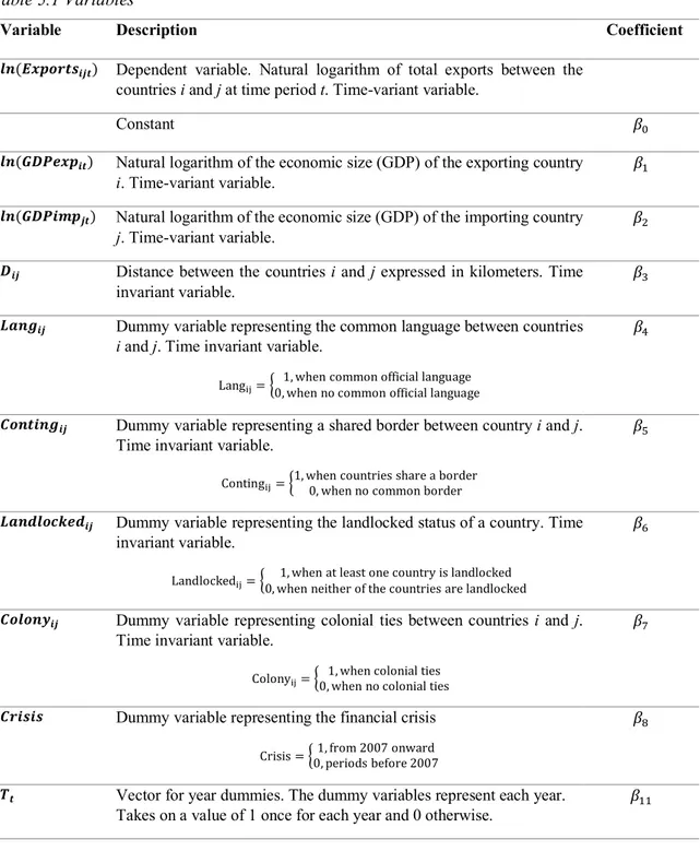
Table 5.1 Variables
Variable Description Coefficient
𝒍𝒏(𝑬𝒙𝒑𝒐𝒓𝒕𝒔𝒊𝒋𝒕) Dependent variable. Natural logarithm of total exports between the
countries i and j at time period t. Time-variant variable.
Constant 𝛽7
𝒍𝒏(𝑮𝑫𝑷𝒆𝒙𝒑𝒊𝒕) Natural logarithm of the economic size (GDP) of the exporting country
i. Time-variant variable.
𝛽<
𝒍𝒏(𝑮𝑫𝑷𝒊𝒎𝒑𝒋𝒕) Natural logarithm of the economic size (GDP) of the importing country
j. Time-variant variable.
𝛽>
𝑫𝒊𝒋 Distance between the countries i and j expressed in kilometers. Time
invariant variable.
𝛽?
𝑳𝒂𝒏𝒈𝒊𝒋 Dummy variable representing the common language between countries
i and j. Time invariant variable.
LangGH= I0, when no common official language1, when common official language
𝛽X
𝑪𝒐𝒏𝒕𝒊𝒏𝒈𝒊𝒋 Dummy variable representing a shared border between country i and j.
Time invariant variable.
ContingGH= I1, when countries share a border0, when no common border
𝛽`
𝑳𝒂𝒏𝒅𝒍𝒐𝒄𝒌𝒆𝒅𝒊𝒋 Dummy variable representing the landlocked status of a country. Time
invariant variable.
LandlockedGH= I0, when neither of the countries are landlocked1, when at least one country is landlocked
𝛽f
𝑪𝒐𝒍𝒐𝒏𝒚𝒊𝒋 Dummy variable representing colonial ties between countries i and j.
Time invariant variable.
ColonyGH= I0, when no colonial ties1, when colonial ties
𝛽h
𝑪𝒓𝒊𝒔𝒊𝒔 Dummy variable representing the financial crisis
Crisis = I0, periods before 20071, from 2007 onward
𝛽l
𝑻𝒕 Vector for year dummies. The dummy variables represent each year.
Takes on a value of 1 once for each year and 0 otherwise.
Table 5.2 EU and EMU Dummy Variables
Variable Description Coefficient
𝑬𝑼𝒊𝒋 EUGH= I1, when at least one country is an EU member
0, otherwise 𝛽q
𝑶𝒏𝒆𝒊𝒏𝑬𝑼𝒊𝒋 OneinEUGH= I1, when one country is an EU member0, otherwise 𝛽<>
𝑩𝒐𝒕𝒉𝒊𝒏𝑬𝑼𝒊𝒋 BothinEUGH= I1, when both countries are EU members0, otherwise 𝛽<X
𝑬𝑴𝑼𝒊𝒋 EMUGH= I1, when at least one country is an EMU member
0, otherwise 𝛽<f
𝑶𝒏𝒆𝒊𝒏𝑬𝑴𝑼𝒊𝒋 OneinEMUGH= I1, when one country is an EMU member0, otherwise 𝛽<l
𝑩𝒐𝒕𝒉𝒊𝒏𝑬𝑴𝑼𝒊𝒋 BothinEMUGH= I1, when both countries are EMU members
0, otherwise 𝛽>7
Table 5.3 Interaction Terms
Variable Description Coefficient
𝑪𝒓𝒊𝒔𝒊𝒔 ∗ 𝑬𝑼𝒊𝒋 The interaction between the Crisis and the EU dummy
vari-ables.
𝛽<7
𝑪𝒓𝒊𝒔𝒊𝒔 ∗ 𝑶𝒏𝒆𝒊𝒏𝑬𝑼𝒊𝒋 The interaction between the Crisis and One in EU dummy
variables.
𝛽<?
𝑪𝒓𝒊𝒔𝒊𝒔 ∗ 𝑩𝒐𝒕𝒉 𝒊𝒏 𝑬𝑼𝒊𝒋 The interaction between the Crisis and Both in EU
dummy variables.
𝛽<`
𝑪𝒓𝒊𝒔𝒊𝒔 ∗ 𝑬𝑴𝑼𝒊𝒋 The interaction between the Crisis and the EMU dummy
variables.
𝛽<h
𝑪𝒓𝒊𝒔𝒊𝒔 ∗ 𝑶𝒏𝒆𝒊𝒏𝑬𝑴𝑼𝒊𝒋 The interaction between the Crisis and One in EMU
dummy variables.
𝛽<q
𝑪𝒓𝒊𝒔𝒊𝒔 ∗ 𝑩𝒐𝒕𝒉𝒊𝒏𝑬𝑴𝑼𝒊𝒋 The interaction between the Crisis and Both in EMU
dummy variables
𝛽><
5.3 Descriptive Statistics
Table 5.4 presents the descriptive statistics for the all OECD and EU countries. To get a more intuitive understanding concerning how the variables differ between the full sample, EU, and EMU, descriptive statistics for the EU and EMU countries have been conducted as well (tables 5.5 and 5.6).
Table 5.5 Descriptive statistics: All EU Countries
Variable Mean Median Standard deviation Minimum Maximum Skewness
𝑬𝒙𝒑𝒐𝒓𝒕𝒔 4.186E+09 4.733E+08 1.185E+10 1.288E+03 1.426E+11 5.361 𝑮𝑫𝑷𝒆𝒙p 5.785E+11 2.388E+11 8.223E+11 7.132E+09 4.030E+12 1.942 𝑮𝑫𝑷𝒊𝒎𝒑 5.785E+11 2.388E+11 8.223E+11 7.132E+09 4.030E+12 1.942 𝑫𝒊𝒔𝒕𝒂𝒏𝒄𝒆 1427.622 1345.486 745.305 59.617 3766.312 0.534
n = 11934
Table 5.6 Descriptive Statistics: All EMU Countries
Variable Mean Median Standard deviation Minimum Maximum Skewness
𝑬𝒙𝒑𝒐𝒓𝒕𝒔 7.735E+09 7.331E+08 1.816E+10 1.288E+03 1.426E+11 3.600 𝑮𝑫𝑷𝒆𝒙𝒑 7.380E+11 2.884E+11 9.424E+11 7.132E+09 4.030E+12 1.508 𝑮𝑫𝑷𝒊𝒎𝒑 7.380E+11 2.884E+11 9.424E+11 7.132E+09 4.030E+12 1.508 𝑫𝒊𝒔𝒕𝒂𝒏𝒄𝒆 1569.793 1600.555 808.919 173.033 3766.312 0.480
n = 3570
When comparing the different groups of countries, it is visible that the sample including all OECD and EU countries shows the highest values for the 𝐺𝐷𝑃𝑒𝑥𝑝, and 𝐺𝐷𝑃𝑖𝑚𝑝. This implies that the OECD and EU countries together consist of the economically largest countries of the sample, as measured by the size of their GDPs. A reason for the total sample displaying the largest values is due to countries such as the U.S. being included. In contrast to the GDP values, the exports are, on average, the largest for the EMU sample countries. As can be expected, the distance variable is lower for both the EU and EMU countries compared to the total sample, as these countries are geographically closer to
Variable Mean Median Standard deviation Minimum Maximum Skewness
𝑬𝒙𝒑𝒐𝒓𝒕𝒔 3.85E+09 3.64E+08 1.57E+10 1.09E+02 3.65E+11 11.560 𝑮𝑫𝑷𝒆𝒙p 1.05E+12 2.88E+11 2.37E+12 7.13E+09 1.86E+13 4.985 𝑮𝑫𝑷𝒊𝒎𝒑 1.05E+12 2.88E+11 2.37E+12 7.13E+09 1.86E+13 4.985 𝑫𝒊𝒔𝒕𝒂𝒏𝒄e 4968.570 2306.526 5137.015 59.617 19586.186 1.226
n = 26520
EU countries, all variables indicate skewness and high standard deviations, implying that heterogeneity is present in the sample. By taking the natural log of the values, skewness and heterogeneity can be reduced. Heterogeneity will be discussed further in the empirical section.
5.4 Correlation Matrix
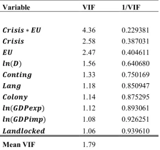
The correlation matrix in Table A.1 in the Appendix presents the Pearson’s correlation coefficient. It can be noted that some of the variables are in fact quite highly correlated with each other, the highest value being 0.79 between the variables 𝐵𝑜𝑡ℎ𝑖𝑛𝐸𝑈 and 𝐶𝑟𝑖𝑠𝑖𝑠 ∗ 𝐵𝑜𝑡ℎ𝑖𝑛𝐸𝑈. However, this is to be expected as the interaction dummy variables are combinations of the different EU, EMU, and crisis dummies. To eliminate the issue of potential multicollinearity, the EU and EMU related dummies along with their inter-action terms with the crisis dummy, will be run in separate regressions. This will result in a total of six different regression models. When the EU and EMU dummies along with the interaction terms between them and the crisis dummy are excluded, the largest value encountered in the matrix, 0.57, is between 𝑙𝑛(𝐸𝑥𝑝𝑜𝑟𝑡𝑠) and 𝑙𝑛(𝐺𝐷𝑃𝑒𝑥𝑝). The correla-tion matrix indicates that an issue of multicollinearity should not be present, as none of the variables, except for the interaction terms, are highly correlated when the EU and EMU dummies are separated.
However, to further confirm that there is no multicollinearity present, a variance inflation factor (VIF) test was conducted for both EU and EMU regression variables. As can be seen in tables A.2 and A.3 in the Appendix, the mean VIF values are 1.79 and 1.59 for EU and EMU, respectively. The highest VIF value for EU regression variables is 4.36 and 3.30 for the EMU regression variables, which indicate that there is no multicolline-arity problem in the variables. As a rule of thumb, a VIF value of 10 or higher might require further investigation (Gujarati and Porter, 2009).
6. Empirical Model and Analysis
6.1 Model
The model used is a differences-in-differences (DID) model. The chosen estimation method is pooled OLS with panel data, as several advantages come with it. With panel data, the sample size increases considerably, and the investigation of more complicated models is enabled. Panel data also studies the dynamics of change better as it is able to combine several cross-sectional observations (Gujarati and Porter, 2009).
According to Angrist and Pischke (2009) DID is a version of a fixed effect method using aggregate data. The DID is used to estimate the effect of a specific treatment through a comparison of the changes in the outcomes over time between a treatment group and a control group. The treatment group experiences the change through an interaction term of an explanatory variable and time dummies. The treatment group is exposed to the ment in one of the time periods, while the control group remains unaffected by the treat-ment during the entire period of the study (Wooldridge, 2002). In this study, the key as-sumption of the DID setup is that the trends in trade would be the same in both groups in the absence of the treatment, which in this case in the financial crisis. We consider the EU and EMU as the treatment groups, while the control groups are the ones defined in the section 5.2.
Pooled OLS assumes that the regression coefficients are the same across all subjects, resulting in no distinction between them. It also assumes that all errors are homoscedastic and independent of each other (Podestà, 2002). The explanatory variables are assumed to be nonstochastic (Gujarati and Porter, 2009). There are disadvantages to this method, as pooled OLS estimates may result in inconsistent estimation of the model if the assump-tions are not fulfilled (Egger, 2002). Furthermore, due to the assumption of homoscedas-ticity, pooled OLS might result in a heterogeneity bias. To control for this, several studies have used a fixed effect approach (Cheng and Wall, 2005).
In recent studies, the Fixed Effects (FE) model has often been employed by economists when estimating gravity equations (Head and Mayer, 2013). The benefit of the FE
ap-other estimators do not consider (Head and Mayer, 2013). There is a major drawback to the fixed effect model, however. The FE estimators cannot obtain coefficient estimates for time-invariant variables, such as distance and common language, which are of interest in a gravity model study (Prehn, Brümmer, and Glauben, 2016; Wooldridge, 2002). Hence, a fixed effect model is not considered useful when it comes to studying these effects (Wooldridge, 2002). As an alternative for the FE model, a random effect model (REM) could be applied. In order for the REM estimates to be consistent and unbiased, several strong assumptions have to be satisfied. One of the requirements is that the error terms are uncorrelated with the independent variables in the model. When it comes to the gravity model, REM is not commonly used due to strong assumptions of heterogeneity in the data. Because of this, the FE and pooled OLS are the dominant methods in gravity model studies (Shepherd, 2013).
The Hausman test can be used to differentiate between the Fixed and Random Effect Models (Wooldridge, 2002). Regarding this study, the Hausman test suggests that FE is the preferred model (Appendix, Table A.8). REM is not considered suitable when the Hausman test is rejected as this would lead to inconsistent coefficient estimates (Gujarati and Porter, 2009). In order to distinguish between pooled OLS and FE, a Wald test was conducted. The results suggest that a fixed effect model is the preferred method for this study (Appendix, Table A.9). However, as the fixed effect model cannot be employed in this study, we use pooled OLS as the base model, but apply the FE model as a robustness test in order to confirm that the pooled OLS provides suitable estimates in this particular study. Pooled OLS has been employed in previous gravity model estimations in several studies, e.g. Rose (2000) and McCallum (1995).
For estimation purposes, the classic gravity equation can be converted into a logarithmic version. The log-log model can be seen in Equation 2.
𝑙𝑛 (𝑇"#) = 𝛽7+ 𝛽<𝑙𝑛 (𝑌"Œ) + 𝛽>𝑙𝑛 (𝑌#Œ) + 𝛽?𝑙𝑛 (𝐷"#) + 𝑢"#Œ
In compliance with the theoretical framework, all empirical models included are based on the general gravity model. However, to better suit the purpose of this study, additional
variables have been included to be able to analyze the relationship between EU or EMU membership and trade during the financial crisis.
Equation 3 displays an augmented gravity model, with the objective to view the overall effects of EU membership. It includes all the independent variables as well as the 𝐸𝑈 dummy, and the interaction term between the 𝐸𝑈 and the 𝐶𝑟𝑖𝑠𝑖𝑠 dummies.
𝑙𝑛Ž𝐸𝑥𝑝𝑜𝑟𝑡𝑠"#Œ• = 𝛽7+ 𝛽<𝑙𝑛 (𝐺𝐷𝑃𝑒𝑥𝑝"Œ) + 𝛽>𝑙𝑛 (𝐺𝐷𝑃𝑖𝑚𝑝#Œ) + 𝛽?𝑙𝑛 (𝐷"#) + 𝛽X𝐿𝑎𝑛𝑔"# + 𝛽`𝐶𝑜𝑛𝑡𝑖𝑔"#+ 𝛽f𝐿𝑎𝑛𝑑𝑙𝑜𝑐𝑘𝑒𝑑"#+ 𝛽h𝐶𝑜𝑙𝑜𝑛𝑦"#+ 𝛽l𝐶𝑟𝑖𝑠𝑖𝑠 + 𝛽q𝐸𝑈 + 𝛽<7(𝐶𝑟𝑖𝑠𝑖𝑠 ∗ 𝐸𝑈) + 𝛽<<𝑻Œ+ 𝑢"#Œ
To further analyze the different aspects of EU membership and trade during the financial crisis, two additional equations will be used. By separating the 𝐸𝑈 dummy, we will be able to analyze whether there appears to be a difference between how the intra-EU and extra-EU trade were affected during the financial crisis. Equation 4 includes all the inde-pendent variables as well as the 𝑂𝑛𝑒𝑖𝑛𝐸𝑈 dummy and the interaction dummy between the 𝑂𝑛𝑒𝑖𝑛𝐸𝑈 and the 𝐶𝑟𝑖𝑠𝑖𝑠 dummies. Equation 5 shows how the intra-EU trade was impacted during the financial crisis by including the variable 𝐵𝑜𝑡ℎ𝑖𝑛𝐸𝑈 and the interac-tion term 𝐵𝑜𝑡ℎ𝑖𝑛𝐸𝑈 ∗ 𝐶𝑟𝑖𝑠𝑖𝑠. 𝑙𝑛Ž𝐸𝑥𝑝𝑜𝑟𝑡𝑠"#Œ• = 𝛽7+ 𝛽<ln (𝐺𝐷𝑃𝑒𝑥𝑝"Œ) + 𝛽>ln (𝐺𝐷𝑃𝑖𝑚𝑝#Œ) + 𝛽?ln (𝐷"#) + 𝛽X𝐿𝑎𝑛𝑔"# + 𝛽`𝐶𝑜𝑛𝑡𝑖𝑔"#+ 𝛽f𝐿𝑎𝑛𝑑𝑙𝑜𝑐𝑘𝑒𝑑"#+ 𝛽h𝐶𝑜𝑙𝑜𝑛𝑦"#+ 𝛽l𝐶𝑟𝑖𝑠𝑖𝑠 + 𝛽<>𝑂𝑛𝑒𝑖𝑛𝐸𝑈 + 𝛽<?(𝐶𝑟𝑖𝑠𝑖𝑠 ∗ 𝑂𝑛𝑒𝑖𝑛𝐸𝑈) + 𝛽<<𝑻Œ+ 𝑢"#Œ 𝑙𝑛Ž𝐸𝑥𝑝𝑜𝑟𝑡𝑠"#Œ• = 𝛽7+ 𝛽<𝑙𝑛 (𝐺𝐷𝑃𝑒𝑥𝑝"Œ) + 𝛽>𝑙𝑛 (𝐺𝐷𝑃𝑖𝑚𝑝#Œ) + 𝛽?𝑙𝑛 (𝐷"#) + 𝛽X𝐿𝑎𝑛𝑔"# + 𝛽`𝐶𝑜𝑛𝑡𝑖𝑔"#+ 𝛽f𝐿𝑎𝑛𝑑𝑙𝑜𝑐𝑘𝑒𝑑"#+ 𝛽h𝐶𝑜𝑙𝑜𝑛𝑦"#+ 𝛽l𝐶𝑟𝑖𝑠𝑖𝑠 + 𝛽<X𝐵𝑜𝑡ℎ𝑖𝑛𝐸𝑈 + 𝛽<`(𝐶𝑟𝑖𝑠𝑖𝑠 ∗ 𝐵𝑜𝑡ℎ𝑖𝑛𝐸𝑈) + 𝛽<<𝑻Œ+ 𝑢"#Œ
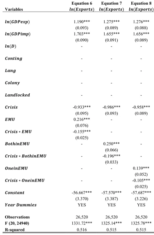
To be able to analyze the relationship between the EMU and trade during the financial crisis, the same models as previously will be used, but the 𝐸𝑈 dummies are replaced with 𝐸𝑀𝑈 dummies. Equation 6 shows the overall impact of EMU membership on trade dur-ing the crisis. It includes all the independent variables as well as the 𝐸𝑀𝑈 dummy and
(3)
(4)
𝑙𝑛Ž𝐸𝑥𝑝𝑜𝑟𝑡𝑠"#Œ• = 𝛽7+ 𝛽<𝑙𝑛 (𝐺𝐷𝑃𝑒𝑥𝑝"Œ) + 𝛽>𝑙𝑛 (𝐺𝐷𝑃𝑖𝑚𝑝#Œ) + 𝛽?𝑙𝑛 (𝐷"#) + 𝛽X𝐿𝑎𝑛𝑔"# + 𝛽`𝐶𝑜𝑛𝑡𝑖𝑔"#+ 𝛽f𝐿𝑎𝑛𝑑𝑙𝑜𝑐𝑘𝑒𝑑"#+ 𝛽h𝐶𝑜𝑙𝑜𝑛𝑦"#+ 𝛽l𝐶𝑟𝑖𝑠𝑖𝑠 + 𝛽<f𝐸𝑀𝑈 + 𝛽<h(𝐶𝑟𝑖𝑠𝑖𝑠 ∗ 𝐸𝑀𝑈) + 𝛽<<𝑻Œ+ 𝑢"#Œ
To study the trade effects when only one of the countries in the country pair is a member of the EMU, Equation 7 is used. Equation 8 displays the intra-EMU effects on trade dur-ing the financial crisis with both countries in the country pair bedur-ing members of the EMU.
𝑙𝑛Ž𝐸𝑥𝑝𝑜𝑟𝑡𝑠"#Œ• = 𝛽7+ 𝛽<𝑙𝑛 (𝐺𝐷𝑃𝑒𝑥𝑝"Œ) + 𝛽>𝑙𝑛 (𝐺𝐷𝑃𝑖𝑚𝑝#Œ) + 𝛽?𝑙𝑛 (𝐷"#) + 𝛽X𝐿𝑎𝑛𝑔"# + 𝛽`𝐶𝑜𝑛𝑡𝑖𝑔"#+ 𝛽f𝐿𝑎𝑛𝑑𝑙𝑜𝑐𝑘𝑒𝑑"#+ 𝛽h𝐶𝑜𝑙𝑜𝑛𝑦"#+ 𝛽l𝐶𝑟𝑖𝑠𝑖𝑠 + 𝛽<l𝑂𝑛𝑒𝑖𝑛𝐸𝑀𝑈 + 𝛽<q(𝐶𝑟𝑖𝑠𝑖𝑠 ∗ 𝑂𝑛𝑒𝑖𝑛𝐸𝑀𝑈) + 𝛽<<𝑻Œ+ 𝑢"#Œ 𝑙𝑛Ž𝐸𝑥𝑝𝑜𝑟𝑡𝑠"#Œ• = 𝛽7+ 𝛽<𝑙𝑛 (𝐺𝐷𝑃𝑒𝑥𝑝"Œ) + 𝛽>𝑙𝑛 (𝐺𝐷𝑃𝑖𝑚𝑝#Œ) + 𝛽?𝑙𝑛 (𝐷"#) + 𝛽X𝐿𝑎𝑛𝑔"# + 𝛽`𝐶𝑜𝑛𝑡𝑖𝑔"#+ 𝛽f𝐿𝑎𝑛𝑑𝑙𝑜𝑐𝑘𝑒𝑑"#+ 𝛽h𝐶𝑜𝑙𝑜𝑛𝑦"#+ 𝛽l𝐶𝑟𝑖𝑠𝑖𝑠 + 𝛽>7𝐵𝑜𝑡ℎ𝑖𝑛𝐸𝑀𝑈 + 𝛽><(𝐶𝑟𝑖𝑠𝑖𝑠 ∗ 𝐵𝑜𝑡ℎ𝑖𝑛𝐸𝑀𝑈) + 𝛽<<𝑻Œ+ 𝑢"#Œ 6.2 Robustness Test
For both the EU and the EMU models, several diagnostic tests were applied to test the credibility of the results. Refer to the Appendix for detailed diagnostics and robustness tests and results. As the data showed signs of first-order autocorrelation as well as heter-oscedasticity, the estimations have been conducted using robust standard errors.
As previously mentioned, an additional robustness test is conducted by estimating the model using a fixed effects approach, despite of the issue of the omitted time-invariant variables. As the fixed effects estimators are always consistent (Gujarati and Porter, 2009), we can use FE to conduct a robustness test to ensure that the obtained results from pooled OLS are robust and sensible. For this robustness investigation, we are mostly in-terested in the values and probabilities of the dummy variables for 𝐶𝑟𝑖𝑠𝑖𝑠, 𝐸𝑈 and 𝐸𝑀𝑈, as well as their interaction terms.
(6)
(7)
6.3 Results
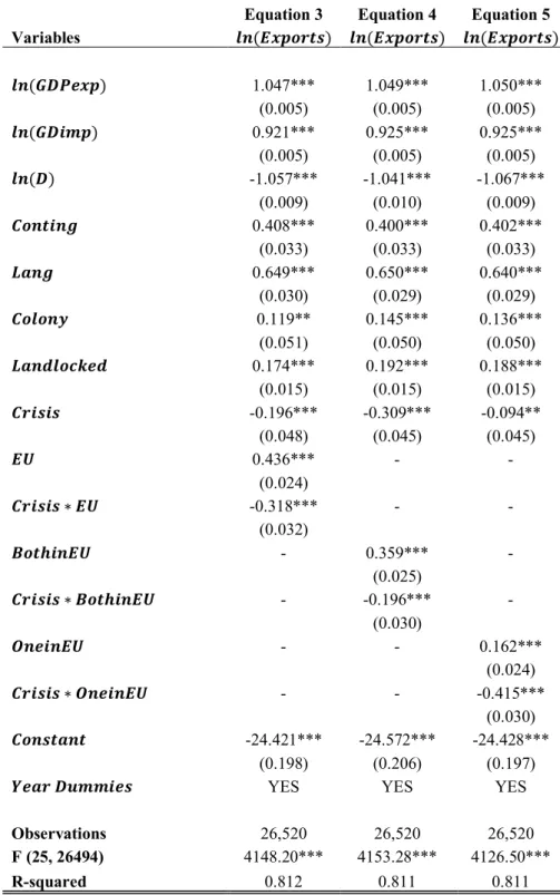
When looking at the regression outputs for EU (Table 6.1) and EMU (Table 6.2), nearly all coefficient estimates are significant at the 1 percent level, while a few are significant at the 5 percent level. For both the EU and EMU regressions, all coefficients except 𝐿𝑎𝑛𝑑𝑙𝑜𝑐𝑘𝑒𝑑 show the expected signs. The estimated models seem to be a good fit as the R-squared values are approximately 0.81 for all of the models. As mentioned, robust standard errors were used to correct for autocorrelation and heteroscedasticity.
Looking at the coefficient estimates in tables 6.1 and 6.2, it is clear that the most funda-mental variables of the gravity model have large effects on trade, which was expected. The GDP of an exporting country and the GDP of an importing country are consistent across all six models for the EU and EMU regressions. The strong negative effect that distance has on trade does not vary greatly between the EU and EMU regression outputs either. The geographical and cognitive distance control variables10 are all significant and
positively related to the trade between countries. Common language appears to have the greatest impact on trade out of all of them.
For the three EU regressions (Table 6.1) the 𝐶𝑟𝑖𝑠𝑖𝑠 coefficient estimates vary between -0.09 and -0.31, indicating that the average effect of the financial crisis was negative for the sample group. The 𝐸𝑈 coefficient of 0.44 is positive, implying that when at least one country from the country pair is a member of the Union, bilateral trade is increased. When one country is a member of the Union, the coefficient value is 0.16, and when both coun-tries of the country pair are EU members, the coefficient value is 0.36, implying that EU membership has a positive effect on trade. The crisis and EU interaction terms are nega-tive for all three equations, which implies an additional neganega-tive effect on trade for mem-ber countries, with the interaction term ranging from about -0.20 to -0.42.
Table 6.1 Regression Coefficient Estimates EU
Equation 3 Equation 4 Equation 5 Variables 𝒍𝒏(𝑬𝒙𝒑𝒐𝒓𝒕𝒔) 𝒍𝒏(𝑬𝒙𝒑𝒐𝒓𝒕𝒔) 𝒍𝒏(𝑬𝒙𝒑𝒐𝒓𝒕𝒔) 𝒍𝒏(𝑮𝑫𝑷𝒆𝒙𝒑) 1.047*** 1.049*** 1.050*** (0.005) (0.005) (0.005) 𝒍𝒏(𝑮𝑫𝒊𝒎𝒑) 0.921*** 0.925*** 0.925*** (0.005) (0.005) (0.005) 𝒍𝒏(𝑫) -1.057*** -1.041*** -1.067*** (0.009) (0.010) (0.009) 𝑪𝒐𝒏𝒕𝒊𝒏𝒈 0.408*** 0.400*** 0.402*** (0.033) (0.033) (0.033) 𝑳𝒂𝒏𝒈 0.649*** 0.650*** 0.640*** (0.030) (0.029) (0.029) 𝑪𝒐𝒍𝒐𝒏𝒚 0.119** 0.145*** 0.136*** (0.051) (0.050) (0.050) 𝑳𝒂𝒏𝒅𝒍𝒐𝒄𝒌𝒆𝒅 0.174*** 0.192*** 0.188*** (0.015) (0.015) (0.015) 𝑪𝒓𝒊𝒔𝒊𝒔 -0.196*** -0.309*** -0.094** (0.048) (0.045) (0.045) 𝑬𝑼 0.436*** - - (0.024) 𝑪𝒓𝒊𝒔𝒊𝒔 ∗ 𝑬𝑼 -0.318*** - - (0.032) 𝑩𝒐𝒕𝒉𝒊𝒏𝑬𝑼 - 0.359*** - (0.025) 𝑪𝒓𝒊𝒔𝒊𝒔 ∗ 𝑩𝒐𝒕𝒉𝒊𝒏𝑬𝑼 - -0.196*** - (0.030) 𝑶𝒏𝒆𝒊𝒏𝑬𝑼 - - 0.162*** (0.024) 𝑪𝒓𝒊𝒔𝒊𝒔 ∗ 𝑶𝒏𝒆𝒊𝒏𝑬𝑼 - - -0.415*** (0.030) 𝑪𝒐𝒏𝒔𝒕𝒂𝒏𝒕 -24.421*** -24.572*** -24.428*** (0.198) (0.206) (0.197)
𝒀𝒆𝒂𝒓 𝑫𝒖𝒎𝒎𝒊𝒆𝒔 YES YES YES
Observations 26,520 26,520 26,520
F (25, 26494) 4148.20*** 4153.28*** 4126.50***
R-squared 0.812 0.811 0.811 *** p<0.01, ** p<0.05, * p<0.1 Robust standard errors in parentheses
Table 6.2 Regression Coefficient Estimates EMU
Equation 6 Equation 7 Equation 8 Variables 𝒍𝒏(𝑬𝒙𝒑𝒐𝒓𝒕𝒔) 𝒍𝒏(𝑬𝒙𝒑𝒐𝒓𝒕𝒔) 𝒍𝒏(𝑬𝒙𝒑𝒐𝒓𝒕𝒔) 𝒍𝒏(𝑮𝑫𝑷𝒆𝒙𝒑) 1.037*** 1.046*** 1.046*** (0.005) (0.005) (0.005) 𝒍𝒏(𝑮𝑫𝒊𝒎𝒑) 0.923*** 0.922*** 0.922*** (0.005) (0.005) (0.005) 𝒍𝒏(𝑫) -1.076*** -1.085*** -1.090*** (0.008) (0.008) (0.008) 𝑪𝒐𝒏𝒕𝒊𝒏𝒈 0.377*** 0.356*** 0.397*** (0.033) (0.033) (0.033) 𝑳𝒂𝒏𝒈 0.622*** 0.620*** 0.644*** (0.030) (0.030) (0.030) 𝑪𝒐𝒍𝒐𝒏𝒚 0.156*** 0.157*** 0.120** (0.052) (0.051) (0.052) 𝑳𝒂𝒏𝒅𝒍𝒐𝒄𝒌𝒆𝒅 0.177*** 0.181*** 0.176*** (0.015) (0.015) (0.015) 𝑪𝒓𝒊𝒔𝒊𝒔 -0.178*** -0.260*** -0.172*** (0.045) (0.044) (0.046) 𝑬𝑴𝑼 0.442*** - - (0.022) 𝑪𝒓𝒊𝒔𝒊𝒔 ∗ 𝑬𝑴𝑼 -0.376*** - - (0.028) 𝑩𝒐𝒕𝒉𝒊𝒏𝑬𝑴𝑼 - 0.397*** - (0.029) 𝑪𝒓𝒊𝒔𝒊𝒔 ∗ 𝑩𝒐𝒕𝒉𝒊𝒏𝑬𝑴𝑼 - -0.338*** - (0.037) 𝑶𝒏𝒆𝒊𝒏𝑬𝑴𝑼 - - 0.273*** (0.023) 𝑪𝒓𝒊𝒔𝒊𝒔 ∗ 𝑶𝒏𝒆𝒊𝒏𝑬𝑴𝑼 - - -0.265*** (0.029) 𝑪𝒐𝒏𝒔𝒕𝒂𝒏𝒕 -24.022*** -24.047*** -24.092*** (0.193) (0.193) (0.194)
𝒀𝒆𝒂𝒓 𝑫𝒖𝒎𝒎𝒊𝒆𝒔 YES YES YES
Observations 26,520 26,520 26,520
F (25, 26494) 4149.21*** 4194.85*** 4091.77***
R-squared 0.812 0.810 0.810 *** p<0.01, ** p<0.05, * p<0.1 Robust standard errors in parentheses
The EMU membership coefficients (Table 6.2) all have a positive effect on trade between the country pairs. The 𝐶𝑟𝑖𝑠𝑖𝑠 variable is negatively related to trade in all three models,
and the EMU dummies, which display the extra trade effect for the EMU member coun-tries during the crisis, is negatively related to trade. For the different EMU models, the interaction term ranges from about -0.27 to -0.38.
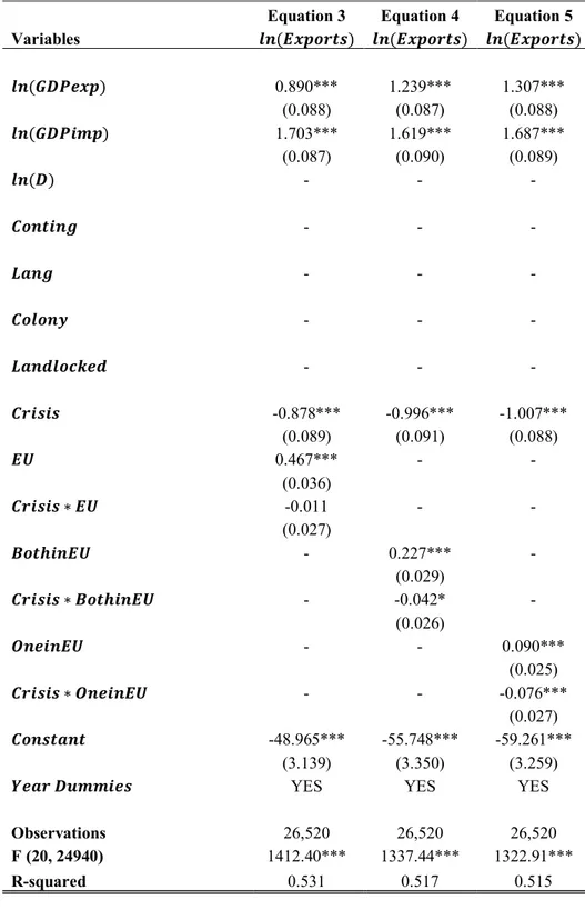
In the fixed effect estimation, all time-invariant variables are omitted (Appendix, tables A.10 and A.11). The coefficient estimates display the same expected signs as the pooled OLS regressions. All estimates, except for the 𝐶𝑟𝑖𝑠𝑖𝑠 ∗ 𝐸𝑈 interaction term, are highly significant. The magnitude of the 𝐶𝑟𝑖𝑠𝑖𝑠 coefficient for both EU and EMU regressions is larger in the FE regression estimates. The crisis and EU as well as the crisis and EMU interaction terms show a smaller additional effect of the crisis, compared to the pooled OLS values. Since nearly all coefficient values are significant and show the same signs as the OLS estimator coefficients, we can conclude that the OLS estimators provide ro-bust results when estimating the models of this study.
6.4 Analysis
The fundamental variables in the gravity model, the distance and the size of the economy, show the expected results in all of the regressions. As the coefficient estimates display relatively large values, they are of great importance as they all have a highly significant impact on the bilateral trade flows. Furthermore, the coefficients are in accordance with the findings from previous studies, which confirm these results (Bun and Klaassen, 2007; Rose, 2000).
Overall, the geographical and cognitive distance control variables show the expected re-sults and are in line with previous studies. The only variable displaying a sign different from the expected sign is 𝐿𝑎𝑛𝑑𝑙𝑜𝑐𝑘𝑒𝑑. This could be due to the fact that EU countries, which make up more than half of the sample in the study, are highly economically inte-grated due to free trade within the Union. It could mean that landlockedness does not limit their trade abilities as much as for countries that are not surrounded by a free trade area, and thus, landlockedness might not pose as many negative effects on countries within the Union. This positive impact of landlockedness in our regressions is in line with earlier studies, which argue that European countries are less impacted by landlockedness than non-European countries (Coulibaly and Fontagné, 2005; Raballand, 2003).