Contingent Hedging : Applying Financial Portfolio Theory on Product Portfolios

(1)

Contingent Hedging

Applying Financial Portfolio Theory on Product Portfolios

Bachelor’s thesis within Business Administration (Finance)

Authors: Viktor Eklöf

Victor Karlsson Rikard Svensson

Tutors: Johan Eklund

Andreas Högberg Jönköping June 2012

(2)

Bachelor’s Thesis in Business Administration (Finance)

Title: Contingent Hedging: Applying Financial Portfolio Theory on Product

Portfolios

Authors: Viktor Eklöf ekvi09im@student.hj.se

Victor Karlsson kavi0999@student.hj.se

Rikard Svensson svri09im@student.hj.se

Tutors: Johan Eklund

Andreas Högberg

Date: 2012-06-21

Subject terms: Finance, Modern Portfolio Theory, Product Portfolios, Black-Litterman,

Efficient Frontier, Investment Decisions, Commodities, Hedging, Risk Management, Contingent Hedge, Diversification, Risk Minimization, Return Optimization, Mining, Metals.

Abstract

In an ever-changing global environment, the ability to adapt to the current economic climate is essential for a company to prosper and survive. Numerous previous re-search state that better risk management and low overall risks will lead to a higher firm value. The purpose of this study is to examine if portfolio theory, made for fi-nancial portfolios, can be used to compose product portfolios in order to minimize risk and optimize returns.

The term contingent hedge is defined as an optimal portfolio that can be identified today, that in the future will yield a stable stream of returns at a low level of risk. For companies that might engage in costly hedging activities on the futures market, the benefits of creat-ing a contcreat-ingent hedge are several. These include creatcreat-ing an optimized portfolio that minimizes risk and avoid trading contracts on futures markets that would incur hefty transaction costs and risks.

Using quantitative financial models, product portfolio compositions are generated and compared with the returns and risks profile of individual commodities, as well as the actual product portfolio compositions of publicly traded mining companies. Us-ing Modern Portfolio Theory an efficient frontier is generated, yieldUs-ing two inde-pendent portfolios, the minimum risk portfolio and the tangency portfolio. The Black-Litterman model is also used to generate yet another portfolio using a Bayesian approach. The portfolios are generated by historic time-series data and compared with the actual future development of commodities; the portfolios are then analyzed and compared. The results indicate that the minimum risk portfolio provides a signif-icantly lower risk than the compositions of all mining companies in the study, as well as the risks of individual commodities. This in turn will lead to several benefits for company management and the firm’s shareholders that are discussed throughout the study. However, as for a return-optimizing portfolio, no significant results can be found.

Furthermore, the analysis suggests a series of improvements that could potentially yield an even greater result. The recommendation is that mining companies can use the methods discussed throughout this study as a way to generate a costless contin-gent hedge, rather than engage in hedging activities on futures markets.

(3)

1 Introduction ... 1

2 Theoretical Framework and Previous Studies ... 3

2.1 Reasons for Diversification ... 3

2.2 Risk Management ... 5

2.3 Modern Portfolio Theory ... 7

2.4 The Black-Litterman Model ... 12

2.4.1 Market View ... 13

2.4.2 Investor Views ... 14

2.4.3 Applications of the Black-Litterman Model ... 14

2.5 Short-term Fluctuations and Long-term Mechanics of Commodity Markets ... 16

2.6 Previous Studies ... 17

3 Methodology and Data Collection ... 21

3.1 Assumptions ... 22

3.2 Modern Portfolio Theory ... 22

3.3 Black-Litterman ... 24

3.3.1 Market view ... 24

3.3.2 Investor Views ... 25

3.3.3 Posterior Portfolio ... 27

3.4 Optimal Portfolio Testing ... 28

3.5 Application to Existing Mining Companies ... 29

4 Results and Analysis ... 30

4.1 Optimized Portfolios vs. Individual Metals ... 30

4.2 Application to Existing Mining Companies ... 34

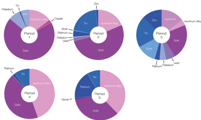
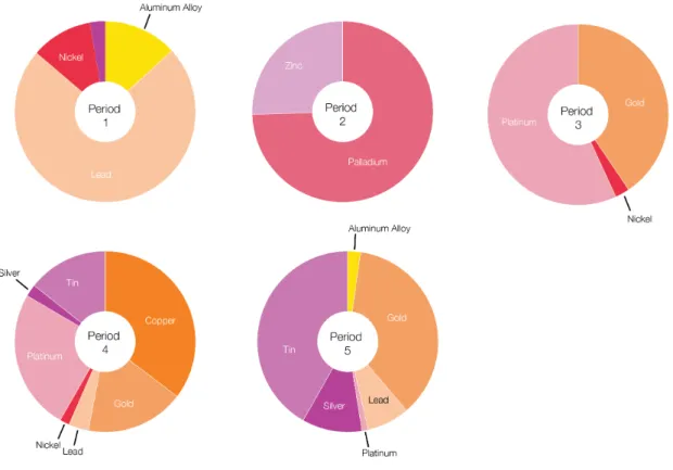
4.2.1 Period 1: From 1996’s Annual Reports ... 34

4.2.6 Summary: Optimized Portfolios vs. Companies’ Portfolios ... 38

5 Conclusion ... 41

6 Drawbacks & Suggestions for Future Research ... 43

6.1.1 Geometric Brownian motion ... 43

6.1.2 The Black-Litterman Model ... 43

6.1.3 Usage by Company Management ... 43

6.1.4 For Future Research ... 44

List of references ... 45

Appendix ... 52

Period 1: Using data from 1993-1996 ... 52

(4)

Period 5: Using data from 2005-2008 ... 68 Minimum variance portfolios of Black-Litterman and

Mean-Variance approaches ... 72

Figures

Figure 2.1. Benefits of diversification. The lower the correlation between asset A and B, the more the investor will benefit from a diversification strategy, as shown by the concave line AB. ... 9 Figure 2.2. Illustration of the efficent frontier. ... 10 Figure 2.3. The efficent frontier and the Capital Market Line. ... 12 Figure 2.4. Bayesian probability. As the number of observations increase,

the posterior return vector is titled further from the prior market view towards the investor view. ... 13 Figure 3.1. Portfolio collection and simulation. The portfolio composition

given by historical data from one time period is simulated on data from the subsequent time period. ... 22 Figure 3.2. The probability distribution of the market view. ... 25 Figure 3.3. The probability of the investor views combined with its

uncertainties. ... 26 Figure 3.4. Creation of the tilted portfolio by blending the quantitative

market view and the investor views. ... 28

Tables

Table 4.1 Comparisons of portfolios’ daily mean return, standard deviation of daily mean returns, return / risk ratio and total return. The

portfolios are obtained using data from September 1 1993 – August 30 1996 (783 trading days). The companies’ portfolios are obtained from 1996’s annual reports. Simulation period: September 2 1996 – September 1 1999 (783 trading days). Risk-free rate, yearly: 4.21%.34 Table 4.2 Comparisons of portfolios’ daily mean return, standard deviation

of daily mean returns, return / risk ratio and total return. The portfolios are obtained using data from September 2 1996 –

September 1 1999 (783 trading days). The companies’ portfolios are obtained from 1999’s annual reports. Simulation period: September 2 1999 – September 2 2002 (783 trading days). Risk-free rate,

yearly: 6.54%. ... 35 Table 4.3 Comparisons of portfolios’ daily mean return, standard deviation

September 2 2002 (783 trading days). The companies’ portfolios are obtained from 1999’s annual reports. Simulation period: September 3 2002 – September 1 2005 (783 trading days). Risk-free rate,

(5)

obtained from 1999’s annual reports. Simulation period: September 2 2005 – September 2 2008 (783 trading days). Risk-free rate,

September 2 2008 (783 trading days). The companies’ portfolios are obtained from 1999’s annual reports. Simulation period: September 3 2008 – September 2 2011 (783 trading days). Risk-free rate, yearly: 3.79%. ... 37 Table A.1 Comparisons of portfolios’ and individual assets’ daily mean

return, standard deviation of daily mean returns, return / risk ratio and total return. The portfolios are obtained using data from September 1 1993 – August 30 1996 (783 trading days). Simulation period:

September 2 1996 – September 1 1999 (783 trading days). Risk-free rate, yearly: 4.21%. ... 55 Table A.2 Comparisons of portfolios’ and individual assets’ daily mean

return, standard deviation of daily mean returns, return / risk ratio and total return. The portfolios are obtained using data from September 2 1996 – September 1 1999 (783 trading days). Simulation period: September 2 1999 – September 2 2002 (783 trading days). Risk-free rate, yearly: 6.54%. ... 59 Table A.3 Comparisons of portfolios’ and individual assets’ daily mean

return, standard deviation of daily mean returns, return / risk ratio and total return. The portfolios are obtained using data from September 2 2005 – September 2 2008 (783 trading days). Simulation period: September 3 2008 – September 2 2011 (783 trading days). Risk-free rate, yearly: 3.79%. ... 71

(6)

Definitions

Contingent Hedge – an optimal portfolio that can be identified today, that in the fu-ture will yield a stable stream of returns at a low level of risk

Risk – defined as the standard deviation of the asset or portfolio

Return – defined as the security’s yield or loss during a certain period of time Long-term – defined as longer or equal to one year (≥ 6 𝑚𝑜𝑛𝑡ℎ𝑠)

Short-term – defined as shorter than one year (< 6 𝑚𝑜𝑛𝑡ℎ𝑠). Studies show that short-term fluctuations pan out towards its long-term equilibrium after 6 months. Financial portfolio / Investment portfolio – a private or institutional investor’s portfolio consisting of the assets acquired

Product portfolio – The product mix of company

Return optimization – To maximize the return for a given degree of risk, as de-scribed by formula 2.5

Risk minimization – to obtain the lowest degree of standard deviation Volatility – See risk

Acknowledgements

We would like to thank several persons who have contributed throughout this study, mainly our tutors Johan Eklund and Andreas Högberg who have provided very useful inputs and feedback. In addition, Daniel Gunnarsson, Business Librar-ian at Jönköping International Business School, has been truly helpful during the data collection process, as well as Joakim Lennartsson at the University Library of Gothenburg. We would also like to express appreciation to colleagues and class-mates for providing inspiration and motivation.

(7)

1 Introduction

In a world of continuous development, planning and forecasting is crucial for managers to make sure that the company can adapt to and exploit the opportunities the future may bring. However, predicting the future is not financial executives’ easiest task, but there are tools that can facilitate this process. Minimizing a company’s volatility, also defined as risk, can be done by reducing the uncertainty about future revenues and thereby simplifying the budgeting and forecasting process. In addition to this, several other benefits come with risk management such as better financing possibilities and decreased costs of financial distress, which in turn will lead to an increased firm value (Smith and Stulz, 1985). The means by which risks can be managed are hedging, insuring and diversifying (Merton, 1993). Hedg-ing, a strategy that involves trading with derivative contracts, and insuring are both com-plex and imply costs as well as risks. Diversification on the other hand can be regarded as a strategy by which a firm can broaden its product offerings to find new market opportuni-ties to increase its revenue and at the same time distribute its risks (Ansoff, 1957). Thus, diversification can lead to the creation of a contingent hedge.

According to Modigliani and Miller (1958), risk management is redundant for a firm to en-gage in since it will not create any values for the shareholders. Instead, the shareholders can themselves manage risks in their own investment portfolios to obtain the wanted degree of risk, leaving risk management to corporate managers superfluously. However, the claims by Modigliani and Miller rest on several strong assumptions, such as perfect markets and no costs of bankruptcy, which have lead to numerous critiques and counter arguments. Incor-porating bankruptcy costs, several studies have shown that by engaging in strategies for hedging and diversification a firm can increase its value, such as Llewellyn (1971) and Levy and Haber (1986). However, the optimal hedge would be a costless hedge, as this would in-crease the firm’s value the most (Smith and Stulz 1985). Therefore diversification, the con-tingent hedge, would be the optimal way to reduce risks to make the firm value surge. But what is the optimal diversification strategy?

The purpose of our study is to examine the possibilities of an implementation of academic portfolio theory developed for financial portfolios on product portfolios in order to find an optimal diversification strategy that minimizes risk while maximizing profits.

Markowitz (1952) presents a model for investors to optimize a financial portfolio in order to maximize returns for a given degree of risk, or simply to minimize risk, by combining

(8)

several securities with certain weights depending on each asset’s return, risk and correlation with other assets. Markowitz’s theory has since been developed several times, by Sharpe (1964) and by Lintner (1965a, 1965b) among others in order to make the model more ap-plicable in practice. The philosophy the authors developep is known as Modern Portfolio Theory and is stilly widely applied both academically and professionally.

Based on the Modern Portfolio Theory, the Black-Litterman model extends beyond quanti-tative finance and provides investors with a way to blend their own views with the return of assets in order to generate a well-diversified financial portfolio to generate optimal fu-ture revenues.

In order to meet the purpose of the study, the following research questions will be scruti-nized:

1. Is it possible for companies to minimize their risks and maximizing their returns by diversification using portfolio theory developed for investors’ financial portfolios on their product portfolios?

2. If so, which of the approaches generates the most risk minimizing and the most op-timal portfolio, the Modern Portfolio Theory or the Black-Litterman model?

These questions are analyzed using 18 years of historical daily prices of 11 metals; alumi-num, aluminum alloy, copper, gold, lead, nickel, palladium, platialumi-num, silver, tin and zinc. By comparing the outcomes from the models with the actual product portfolios of six real world mining companies, the efficiency of these models are examined.

The structure of this paper is as follows. It begins with a brief explanation of the empirical findings and theories behind diversification and risk minimization and is followed by the framework behind Modern Portfolio Theory and the Black-Litterman model. Subsequently, previous studies on the use of portfolio theory on product portfolios are presented. In the methodology section, the approach that is used for collecting and analyzing the data is de-fined and explained. In the following section the results are presented and analyzed and thereafter concluded in the final section.

(9)

2 Theoretical Framework and Previous Studies

In a reality ruled by the findings of Modigliani and Miller (1958), neither capital structure, nor risk minimization, nor diversification is useful for companies since this will not lead to increased values for the shareholders. However, numerous studies refute these statements. As for financial portfolios, the fact that diversification can be used for risk minimization is well recognized and several developments have been made since the first outlines of the modern portfolio theory were drawn by Markowitz (1952). Still the concept and its devel-opments are used widely.

2.1 Reasons for Diversification

Modigliani and Miller (1958) claim that the capital structure of a firm is uncorrelated to the market value of the firm. Contrary to previous theory, increasing the firm’s leverage will not generate any benefits for its shareholders as these can instead simply increase the lever-age in their own investment portfolios by buying on margin. Investors can also undo the leverage of a company by acquiring an equal amount of the firm’s securities and debt. Therefore a company cannot increase its market value simply by increasing the leverage and its shareholders will not be better off if this is done. By the same token, a merger be-tween two companies is superfluously and will not lead to a market value greater than the sum of the two firms’ individual market value ex ante the merger. The reason for this is that investors can prior to the merger merely buy shares from the two companies and thereby artificially create a merger in their private investment portfolios that will provide the investors with the same benefits as a real world merger would do. If the two firms merge, this will not generate any benefits for the investors and consequently the company management cannot expect a premium in the market value compared to the sum of the two firms individually. The same argument goes for the diversification of product portfo-lios. A company selling one product will not be able to increase its market value by starting to sell another product, even if the demand of the two products are uncorrelated, since in-vestors could purchase shares from one firm selling one of the products and from another firm selling the other product. Investors would then be able to reap the benefits from a di-versified product portfolio and will not be better off if one of the firms decides to sell the other product as well.

Several assumptions are made by Modigliani and Miller (1958). These include that markets are perfect and of atomistic competition, which implies that the market consists of several

(10)

small firms without market power, that economies of scale does not exist, that there are no entry costs, that firms are price takers and that prices as well as profits are low. In addition, assumptions are made that there are no costs of bankruptcy and that neither taxes nor asymmetric information exist. The authors also assume that a company’s common stock will generate profits indefinitely. These strong assumptions in combination with the results Modigliani and Miller present have lead to numerous critiques. Stieglitz (1969) criticizes the implicit assumption that a bond of one firm with a low debt-equity ratio is indistinguishable to a bond of another firm with a high debt-equity ratio. These two bonds will yield differ-ent returns. In addition, when the risk of bankruptcy exists, the returns from bonds will be inconstant. Smith (1970, 1972) shows that in a world where the risk of bankruptcy is pre-sent Modigliani and Miller’s theorems do not hold. The amount of company leverage can-not be completely adjusted by individual investors through modifications in their private investment portfolios, such as by buying on margin or “undoing” leverage by purchasing equal amounts of a corporation’s stocks and bonds. If the rate of return of a company’s in-vestments is lower than the rate of interest on its debts, there exists a risk of default. Fur-thermore, if there were no risk of default, there would not be any difference between dif-ferent corporate bonds, bonds issued by the U.S Treasury and a savings account with the same maturity. Smith (1972) concludes that in corporate finance one cannot simply omit bankruptcy and that therefore the assertions by Modigliani and Miller cannot be seen as valid.

The claim that company diversification through conglomerates and product diversification is irrelevant has been criticized severely. Lewellen (1971) proves that firms diversifying their operations reduce the risk of running bankrupt. The same is said for lenders who can re-duce the risk of bankruptcy by diversifying among borrowers. When these two are com-bined, hence when a lender diversifies and finances several companies that all are all diver-sified, both actors’ risk of default is reduced. Levy and Sarnat (1970) argue that diversifica-tion by mergers can imply financial advantages for companies. These advantages include increased access to capital markets as well as lower financing costs; this because diversifica-tion leads to decreased risk of bankruptcy. Diamond (1984) discusses the benefits that come with diversification for independent projects, where the income from the different projects can be cross-pledged. This is useful when raising new capital, since one project’s revenues can be used as collateral for another project. Levy and Haber (1986) stress that when uncertainties regarding future demand and profitability from goods exist,

(11)

diversifica-tion in the product portfolio leads to increased expected returns. Amihud and Lev (1981) argue that in manager-controlled firms motivations to reduce the risk can be caused by the incentives of the company management. In this type of companies, by diversifying in the product portfolio, the risk of the firm’s income can be minimized and as a result manage-ment’s employment risk is reduced. As for owner-controlled firms, the incentives to con-glomerate acquisitions and diversification of product portfolios are not as strong since the owners might hold shares in other companies as well and thereby they diversify their own investment portfolios. Company managers on the other hand might earn their entire in-come from one single firm, and are therefore naturally more risk averse since all of their earnings depend on that of the company (Amihud and Lev, 1981).

2.2 Risk Management

In a Modigliani and Miller type of world, even risk management is pointless. However, this is based on strong assumptions as well, assumptions that may not be valid in the real world. Merton (1993) mentions three ways to manage risk; by hedging, insurance and diversifica-tion. Most of the research on the topic of risk management is about hedging. Smith and Stulz (1985) argue that hedging by companies will increase the firm value, as long as the hedging cost does not exceed the gains. The hedging can be done in various ways and af-fects the firm value through either taxes, contracting cost or the hedging policy’s effect on the investing decision. By hedging, a company can reduce the variability of its own value, which will result in a lower risk of having to face bankruptcy costs. An investment in a hedged financial portfolio can also reduce the potential bankruptcy costs, which would yield positive returns if the corporation were to face bankruptcy when lending is unattaina-ble. In turn this will benefit the shareholders who face less risk of losing their invested money in addition to the increased firm value of the hedged company. Even incomplete hedging, meaning that not all future cash flow insecurities are being covered for, will in-crease the value of a firm. However, the costs have to be accounted for since some hedging tend to be very expensive; something shareholders have to account for before making an investment (Smith and Stultz 1985).

Froot, Scharfstein and Stein (1994) find evidence for the usefulness of hedging when it is more expensive for a firm to raise external financing than internal. The authors argue that complete protection from risk is not the best hedging strategy in general. Still, a company should protect itself from some risk exposure since this can increase the value of the firm

(12)

by implying less variability in cash flows that can stabilize investment and financing plans. A disruption in these plans can lead to high costs that can be avoided to some extent by risk management. In addition, without hedging, a firm may have to forgo profitable in-vestment opportunities because of expensive external financing. Furthermore, the authors state that by using futures contracts, the firm may face extremely large margin calls and therefore that forwards are to prefer. However, the usage of forward contracts implies a credit risk and therefore no large positions should be taken in these contracts.

Mello and Parsons (2000) claim that a company with no financial constraints will not be better off by hedging, while a company with financial constraints has a lot to gain by hedg-ing, gains including reduced external financing expenses that make potential profitable in-vestments possible. However, the hedge needs to be adequately constructed, otherwise it may even reduce the firm’s value. By a proper hedging strategy, the financially constrained firm will be able to smoothen out the revenues from one period to another and reduce its costs for bankruptcy and thereby increase its value.

Stulz (1990) argues that if a firm diversifies among projects, the shareholders will benefit from the less volatile cash flow the diversification implies. Thus diversification can increase the wealth of shareholders. The same goes for hedging, Stulz claims. This is likely because of asymmetric information between shareholders and company management.

Fender (2000) stresses that the existence of asymmetric information on financial markets makes companies pursue hedging strategies by acquiring derivative contacts in order to manage risk. However, because of transaction costs, basis risk and counterparty risk, these hedging strategies may be superfluous.

Tufiano (1996) proposes alternatives to hedging. Using diversification, a firm can spend less time on managing financial risks and therefore diversification should be considered to some extent as a substitute to hedging.

Ansoff (1957) describes four ways for firms to develop their product offerings; market penetration, market development, product development and diversification. Diversification differs from the others, since it can lead to a situation where the firm needs to make organ-izational and operational changes. The reasons for diversification are several, such as to modernize outdated technology, to reinvest earnings and to spread the risks. As a result of the distribution of risks, diversification can stabilize a firm’s revenue and thereby simplify

(13)

planning and forecasting. A product portfolio consisting of several different products will make the firm less sensitive to negative events that cannot be predicted, such as economic recessions, technological breakthroughs or natural disasters. Furthermore, diversification can lead to company growth because of an increase of potential customers.

2.3 Modern Portfolio Theory

Since the seminal work by Markowitz (1952) on modern portfolio theory and diversifica-tion, investors have sought a properly diversified portfolio with minimum risk and maxi-mum excess returns. Markowitz introduces the theory that by diversifying the assets it is possible to get a portfolio with a higher return for taking on a lower degree of risk. Marko-witz presents a model called expected returns – variance of returns rule, or just E-V rule. If R is the return of the portfolio, then V(R) is the variance of returns of the portfolio, de-fined as: 𝑉 𝑅 = 𝑤_!𝑤_!𝜎_!" ! !!! ! !!! (2.1) where

𝑉 𝑅 is the variance of returns of the portfolio 𝑤_! is the weight in the portfolio of the i:th asset 𝑤! is the weight in the portfolio of the j:th asset

𝜎_!" represents the covariance between asset i and asset j

The formula for covariance between the return of asset i and asset j can be expressed as:

𝜎_!" = 𝜌_!"𝜎_!𝜎_! (2.2)

where

𝜌_!" represents the correlation between the returns of asset i and asset j

𝜎! is the standard deviation of returns for asset i

(14)

The formula for correlation between the return of asset i and asset j can be expressed as:

𝜌_!" =𝐸[ 𝑖 − 𝜇! 𝑗 − 𝜇! ]

𝜎_!𝜎_! (2.3)

where

𝜇_! is the mean of asset i 𝜇_! is the mean of asset j

𝜎_! is the standard deviation of returns for asset i. 𝜎_! is the standard deviation of returns for asset j. The return R of the portfolio is expressed as:

𝑅 = 𝑤_!𝑅_! (2.4)

where

𝑅_! is the return of the i:th asset and is a random variable

𝑤_! is the weight of that asset relatively to the entire portfolio and is decided upon by the investor (Σ wi = 1).

According to Markowitz (1952), the investor can choose between several combinations of return and risk by choosing different weights of the assets. Furthermore, Markowitz argues that the E-V rule will give a number of efficient portfolios, the highest possible return for the lowest possible risk, the majority of these are diversified. However, a portfolio cannot only be diversified in order to be efficient, it needs to be diversified correctly. Doing this, the risk will not be eliminated completely, but minimized.

To find all efficient portfolios available that maximize the return for the degree of risk tak-en on would be a tedious process. Every set of efficitak-ent portfolios can be explained by a set of corner portfolios and since there might be an infinite number of efficient portfolios, there are a definite number of corner portfolios. Since an efficient portfolio necessarily does not need to contain all assets, corner portfolios can be found where new assets are added or removed to the portfolio when moving along the E-V curve. For every point on this curve there is a unique relationship between the weights of the assets in the efficient

(15)

portfolio and the ratio between the return and the risk. By combining sets of corner portfo-lios it is possible to reach any point on the E-V curve (Sharpe, 1961).

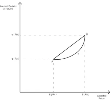
Sharpe (1964) develops Markowitz’s theory further, perhaps as a result of the deeply theo-retical approach that impregnated the paper. Furthermore, Markowitz only uses a portfolio combined of two assets, while Sharpe uses several; consequently Sharpe’s approach makes it easier for investors to implement the theories in practice. There are two different types of risk to be found among assets, a systematic component as well as an unsystematic compo-nent. The systematic risk is a risk caused by the market that all assets are subject to and that cannot be avoided by diversification. However, unsystematic risk can be removed by diver-sification. Therefore there exists a positive relationship between return and systematic risk among assets, which is the risk premium. Proper diversification can make investors remove all risk except for that caused by fluctuations in the economy, and only assets’ sensitivity to these fluctuations are useful when determining the level of risk the asset is subject to. An investment would be efficient if there for the same level of return are no investments with a lower degree of risk or for the same level of risk are no investments with a higher level of return. By diversification among assets, some of the risk can be avoided, how much depends on the correlation between the assets. This is shown in Figure 2.1, where points A and B represents two different assets. Point Z represents a portfolio consisting of these two assets. The lower the correlation between asset A and asset B, the more concave the curve between asset A and B, hence the more risk can be removed by diversification.

Figure 2.1. Benefits of diversification. The lower the correlation between asset A and B, the more the investor will benefit from a diversification strategy, as shown by the concave line AB.

(16)

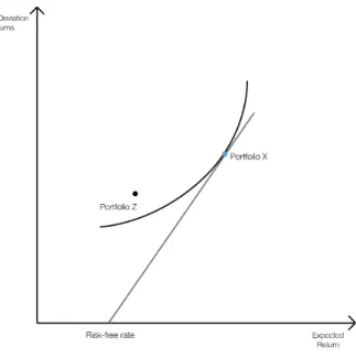
By introducing risk free assets to the model, which is an investment that offers a certain re-turn with a variance of zero, combinations of riskless assets and risky assets are found on a straight line as seen below. This line is the Capital Market Line. As seen in Figure 2.1, by investing in risk free assets as in point where the CML intersects the X-axis, and in risky as-sets as in Portfolio X, all investment combinations on the line are attainable. One combina-tion would be seen as the efficient and dominate the other combinacombina-tions. This combinacombina-tion is located on the Capital Market Line that intersects with the investment opportunity curve, which is the curve that contains all combinations of risky assets and consists of the numer-ous corner portfolios. Portfolio Z will always be dominated by Portfolio X, which is the tangent portfolio (Sharpe, 1964).

Figure 2.2. Illustration of the efficent frontier.

Lintner’s (1965a) developments originate from the concepts as described above, but are explained more in-depth and uses more assets than the previous studies. The relative size of risky investments versus risk-free investments is irrelevant when deciding the composi-tion of risky assets. This implies that the wealth of investors does not affect the relative size of risky assets in their portfolios. To find the optimal portfolio, is the one for which θ is maximized in the formula:

𝜃 = !ℎ!𝑥!

( _!"ℎ_!ℎ_!𝑥_!")(!!) (2.5)

ℎ! is the weight of asset i in the portfolio, !ℎ! = 1

(17)

𝑥_!" is the variance 𝜎!!"# when i = j and covariances when i ≠ j

To find the optimal weight of each asset in the portfolio, Lintner (1965a) proposes the fol-lowing formula:

ℎ_!! ₌ 𝜆!

𝜆! − _!!!ℎ!!𝑥!"/𝑥!! (2.6)

and

𝜆_! = 𝑥_!/𝑥_!! (2.7)

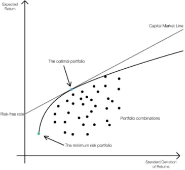
One may believe that stocks whose expected return is less than that of the risk-free rate, that is with a negative risk premium, would be excluded from an efficient portfolio; this is, however, not the case. Lintner (1965a) shows that even though some risky assets might be outperformed by risk-free assets, they are still valuable to hold long in the portfolio if they have a negative correlation with the other assets in the portfolio. By adding such stocks to a portfolio, investors are able to decrease the total variance of the portfolio’s return. There-fore Lintner (1965a) concludes that the presumption about the relation between risk pre-mium and the standard deviation of the asset’s return only is relevant when investors choose between a risk-free asset and one single risky asset, not when investors choose as-sets to an efficient portfolio. Therefore the variance and covariance with other asas-sets is the most suitable measurement of risk, these two variables will eventually decide each asset’s weight in the portfolio. As can be seen in Figure 2.3, a number of different combinations of assets create several portfolios, but only the ones on the efficient frontier are regarded as efficient. The optimal portfolio, or the tangent portfolio, is the one located where the Capi-tal Market Line is tangent to the efficient frontier; this is the portfolio where equation 2.5 is maximized (Lintner, 1965b).

(18)

Figure 2.3. The efficent frontier and the Capital Market Line.

Hence, the effects of diversification are important to a large extent, as Lintner concludes ”the added return available on the optimal portfolio will always more than compensate for the extra risk involved in holding it … and this optimal portfolio, by definition, is the one offering the best diversification” (Lintner, 1965b, p. 610). The minimum risk portfolio is located on the very left of the efficient frontier.

2.4 The Black-Litterman Model

Black and Litterman (1992) present a model to generate better inputs for portfolio optimi-zation. They argue that quantitative portfolio optimization methods when unconstrained generate extreme portfolios with large short positions in certain assets and large long posi-tions in assets with low market capitalization. Jones, Lim and Zangari (2007) state that prior to the development of the Black-Litterman model investors were not satisfied with the sometimes unreasonable and extreme portfolios that previous portfolio optimization niques generated. This led investors to forego the benefits of portfolio optimization tech-niques, or constrain the process so that the solution was to a large extent predetermined. The insight of Black and Litterman (1992) is that the extreme portfolios generated by port-folio optimization techniques were not necessarily a fault in the theory, but rather due to feeding the optimization process flawed risk and return inputs. Lee (2000) and Drobetz

(19)

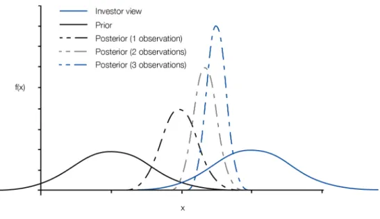
(2001) argue that the Black-Litterman model to a large extent mitigates the negative effects caused by estimation errors generated by previous portfolio optimization techniques. Building upon the existing theories within portfolio optimization, Black and Litterman (1992) develop a Bayesian approach to asset selection. The model blends a quantitative portfolio optimization process with the views of investors on the performance of individu-al assets or asset classes.

Figure 2.4. Bayesian probability. As the number of observations increase, the posterior return vector is titled further from the prior market view towards the investor view. Figure 2.4 indicates how the Black-Litterman model incorporate investor views; it tilts the quantitative market view generated towards the portfolio suggested by investor views. In effect, as the number of observations of investors with the same view grows, the posterior portfolio is tilted further towards the investor view.

2.4.1 Market View

The other component of the model is a quantitative market view. According to Idzorek (2002) the implied equilibrium returns are defined as:

Π = 𝜆Σ𝑤_!"# (2.8)

where

Π is the Implied Excess Equilibrium Return Vector (N × 1 column vector) 𝜆 is the risk aversion coefficient (the expected risk-return tradeoff)

(20)

Σ is the covariance matrix (N × N) of excess returns

𝑤_!"# is the market capitalization weighting factor (N × 1 column vector)

Idzorek (2002) further defines the risk aversion coefficient by the formula:

𝜆 = 𝐸 𝑟 − 𝑟_! 𝜎! _(2.9)

where

𝐸 𝑟 is the expected return

𝑟! is the return of the risk-free asset

𝜎! _{is the variance of the asset}

2.4.2 Investor Views

Jones et al (2007) state that a view is a forecast about an investment’s future risk and re-turn. With the equilibrium expected returns, an investor with private views on the future development of a certain asset can use this in the Black-Litterman model to generate a portfolio based on that view. Using the covariance matrix, the covariance of assets blends the implied excess return vector with the views of investors to generate balanced portfoli-os. These portfolios are tilted relative to the risk-aversion and the confidence of the private views of a particular investor.

2.4.3 Applications of the Black-Litterman Model

In the original article, Black and Litterman (1990) demonstrate how the model can be im-plemented using data from global bond markets. A follow-up article applied the model to three asset classes (currencies, bonds and equities) on 7 international markets (Germany, France, Japan, United Kingdom, United States, Canada and Australia) (Black and Litter-man, 1992).

Following the model described by He and Litterman (1999), Walters (2009) suggests that the new posterior combined return vector is calculated as:

E[R] = Π + 𝜏 Σ 𝑃!_{𝑃 𝜏 Σ 𝑃}! _{+ Ω}!! _{𝑄 − 𝑃 Π} _(2.10)

(21)

𝐸 𝑅 is the Combined Return Vector (N × 1 column vector)

Π is the Implied Equlibrium Return Vector (N × 1 column vector) 𝜏 is a scalar

Σ is the covariance matrix of excess returns (N × N matrix)

𝑃 is a matrix to identify the assets with views (K × N matrix, where K is the number of views and N is the number of assets.

Ω is a diagonal covariance matrix of error terms from the expressed views rep-resenting the uncertainty in views (K × K matrix where K is the number of views)

𝑄 is the view vector (K × 1 column vector)

According to Idzorek (2002) the value for the scalar 𝜏 is difficult to set, and there are nu-merous studies that all use different values for 𝜏. According to Blamont and Fioozye (2003) this scalar is the standard error of estimate; this scaling factor diminishes as the number of observations increase. Walters (2009) suggest using the formula 𝜏 = _!!!! where T is the number of samples and k is the number of assets. He and Litterman (1999) use a 𝜏 of 0.05. The Black-Litterman model also generates a posterior covariance matrix based on the tilted portfolio. He and Litterman (1999) and Walters (2009) calculate the posterior covariance matrix as:

Σ_! = Σ + 𝜏 Σ !!_{+ P}!_Ω!!_𝑃 !! _(2.11)

where

Σ_! is the posterior covariance matrix (N × N matrix)

Σ is the covariance matrix of excess returns (N × N matrix) 𝜏 is a scalar

𝑃 is a matrix to identify the assets with views (K × N matrix, where K is the number of views and N is the number of assets.

(22)

Ω is a diagonal covariance matrix of error terms from the expressed views rep-resenting the uncertainty in views (K × K matrix where K is the number of views)

The posterior combined return vector E[R] and the posterior covariance matrix Σ! could

be used as inputs to generate the efficient frontier directly, also Walters (2009) calculates the weights of the optimal tilt portfolio as:

w = Π(Δ Σ_!)!! _(2.12)

where

𝑤 is the posterior weights of the optimal tilt portfolio (1 × N column vector) Π is the Implied Equlibrium Return Vector (N × 1 column vector)

∆ is a scalar representing the global risk aversion coefficient Σ! is the posterior covariance matrix (N × N matrix)

2.5 Short-term Fluctuations and Long-term Mechanics of

Commodity Markets

Black (1976) develops the one-factor cost-of-carry formula, which is the basis for futures pricing. The formula assumes a risk-neutral world where the only source of uncertainty is the spot price of the underlying asset (Hilliard and Reis, 1998). The one-factor cost-of-carry formula can be calculated as 𝐹! = 𝑆!𝑒(!!!)!, where 𝛿 is the convenience yield. Hilliard and

Reis (1998) as well as Schwartz and Smith (2000) define the convenience yield of a com-modity as the premium the seller obtains from storing the comcom-modity that cannot be ob-tained when simply owning a futures contract on the same commodity.

According to Schwartz and Smith (2000) the spot price of commodities are subject to two different stochastic processes depending on the time horizon. In the long-run commodities are assumed to develop according to a Geometric Brownian motion. In the short-run the commodity spot prices are assumed to follow an Ornstein-Uhlenbeck process. The

(23)

Ornstein-Uhlenbeck process is a stochastic mean reverting process that reverts to an equi-librium price generated by the Geometric Brownian motion.

Geman (2005) defines the Geometric Brownian motion as a stochastic process St, which is

governed by the stochastic differential equation, which is calculated by: 𝑑𝑆!

𝑆_! = 𝜇𝑑!+ 𝜎𝑑𝑊! (2.13)

where

𝜇 is the constant drift of the Geometric Brownian motion 𝜎 is the constant volatility of the asset

𝑊_! is the standard Wiener process

Black (1976) states that there is no reason to believe that the price of futures contract would be a reliable indicator of the future spot price. He further expresses that “the spot price of an agricultural commodity tends to have a seasonal pattern: it is high just before a harvest, and low just after a harvest. The spot price of a commodity such as gold, however, fluctuates more randomly” (p. 167). The Geometric Brownian Motion assumes a constant drift rate (Hilliard and Reis, 1998). Therefore the applications to the commodity market would be limited to commodities with a clear bull and bear market trend rather than those subject to yearly cyclical trends such as agricultural commodities.

2.6 Previous Studies

Some studies have indicated that the use of financial portfolio theory can be used for other purposes than when composing financial portfolios. It has been applied for the analysis of product portfolio compositions, and for the analysis of commodities. However, sparsely of research have been made on this topic.

Cubbage and Redmond (1988) use Sharpe’s (1964) developments of the Modern Portfolio Theory to retrieve the price of timber from yearly prices of stumpage (price for the right to harvest timber) between 1951 and 1985 and added the growth rate changes. The same the-oretical framework is also used by Barry (1980) in his risk and return analysis of agricultural land in the period between 1950 and 1977. Using a mixture of stocks, bonds and farm real estate index, and weighting the outstanding market values against the annual return each

(24)

year; he concludes that Modern Portfolio Theory is applicable for portfolio analysis of in-vestment and that farm real estate is a promising resource to include in a well-diversified portfolio in order to decrease risk. Another known example is Holthausen and Hughes (1978) and their work, where Modern Portfolio Theory is used for the estimation of prices for beef, hogs, corn, eggs, poultry, soybeans and other food commodities. Holthausen and Hughes found theoretical difficulties for the application of the theory for commodities. They argue that the seasonal harvesting of a specific commodity cause variability over time in supply, they also stress that some commodities have storage cost and that commodities some times are being held as inventory as a security for future production targets. This is in line with the claims of Black (1976). Furthermore Holthausen and Hughes find that a secu-rity market index is representing the global capital market poorly when studying commodi-ties. As a result of the reasons mentioned they conclude that the use of MPT is less feasible for commodities than securities.

One field on which Modern Portfolio Theory has been used to a somewhat large extent is forestry. Mills and Hoover (1982) use portfolio theory in their research of hardwood for-estland in the Midwestern United States, which results in improved returns and reduced risk in their investment portfolio. Fortson (1986) uses a generalist approach when investi-gating whether MPT can be applied for forestry investments. He concludes that by using MPT that there are great advantages in forest products since they can handle long-term debt and account for a relatively low risk. Olsen and Terpstra (1981) investigates the spot market for softwood logs in Oregon between 1968 and 1978 by using MPT and the results prove that combinations can be found with the similar yields as U.S. T-bills.

Wind (1974) studies if modern portfolio theory can be used as a tool for decision of prod-uct portfolios for companies. Several studies including Gup (1977) and Cardozo and Smith (1983) state that using financial portfolio models for product portfolios and product mix is an interesting topic and warrants future research, even though no significant conclusions are drawn.

According to Wind (1974), “An ‘optimal’ product mix is achieved when a company for a given level of risk cannot improve its profits (or any other objective) by deleting, modifying or adding products” (p. 463). The main idea with this type of portfolio theory is to mini-mize the risk and maximini-mize the profit. Thus it is the same concept, which is used within stock portfolio allocation (Wind 1974). According to the concepts of financial portfolio

(25)

theory, a dominant theory is to prefer, meaning either a portfolio yielding maximum return or minimum risk. These concepts are proven to be more efficient than so called middle-of- the-road theories with an unclear positioning (Cardozo and Smith 1983). Wind (1974) pre-sents another theory of portfolio analysis. It states that it is in fact both theoretically and operationally feasible to use information about each existing or potential product, such as expected return, variance and the relationship with the other products returns. When using this information in an analysis, one can identify efficient portfolio combinations. This is in line with the claims by Markowitz (1952), Sharpe (1964) and Lintner (1965a, 1965b). Wind (1974) argues further that there are alterations between products and securities, which have to be taken into account when talking about portfolio theory in general. First and foremost securities will always be available for sale and with a given level of risk ap-plied, while certain products, which are calculated to be efficient alternatives for a portfolio might not be offered by the specific company of interest, that also prove to lack resources and competences needed within the specific field. To implement the new product into the production will be costly and hence change the original financial conditions. Another diffi-culty when applying portfolio theory on product portfolios is that the required quantity of the desired product might not be available and will affect the calculations in a negative manner.

In the empirical study conducted by Cardozo and Smith (1983), the authors stress that product-market investments show great positive covariance within return and risk meas-urements and hence can be great alternatives for the type of profit maximizing theories constructed for financial portfolios. The results gathered from the models should give stra-tegic management an important tool while designing and managing their product portfolios in order to be more efficient.

The systematic risk is something that all stocks and products face. Therefore it is not pos-sible to eliminate the entire systematic risk component through diversification, but by dif-ferentiating the portfolio one can eliminate the so called unsystematic risk, which is linked to a single unforeseeable event, such as a storm, a fire or a bad corn harvest which will af-fect only a company, industry or single product (Gup 1977). This is also in line with the ar-guments of Markowitz (1952), Sharpe (1964) and Lintner (1965a, 1965b).

Berck (1981) studies how farmers can use agricultural futures to a greater extent. The arti-cle states that a survey by the Commodity Futures Trade Commission shows that merely

(26)

5% of farmers directly participate in the futures market. Berck (1981) derives a model for production planning based on several factors, including the historical yield of a particular agricultural commodity, the yield of the futures prices for the same commodity and the cost of producing that commodity. The author concludes that diversification greatly bene-fits the farmers, as it reduces the variance of the entire portfolio and significantly improves the mean-variance trade-off. Furthermore, Berck concludes that the costs of hedging for producers of agricultural commodities are too high to be worthwhile. Berck (1981) also studies the effects of debt on the production of agricultural commodities and concludes that fixed debt leads to the selection of a riskier risk-return plan.

Black (1976) state that there is no reason to believe that the price of a commodity future should be a good indicator of the future spot price of that same commodity. Schwartz and Smith (2000) provide a mathematical model, which shows that the spot prices of commodi-ties are assumed to trade at levels higher than those of the futures; because of a risk-premium benefitted to the holder of the risky asset. Berck (1981) also concludes that the construction of a yield-predicting model for agricultural commodities should be construct-ed in such a manner, so that the prconstruct-edictions are not basconstruct-ed entirely on futures prices.

(27)

3 Methodology and Data Collection

For this study, historical closing spot prices has been collected from ThomsonReuters DataStream for aluminum, aluminum alloy, copper, gold, lead, nickel, palladium, platinum, silver, tin and zinc from September 1, 1993 to September 2, 2011. These 18 years of data is used to find optimized portfolios and test their future returns and volatility. Using daily closing prices gives the most accurate results because of the larger sample it provides (Ruppert, 2004). In addition, daily historical closing prices have been used when testing Modern Portfolio Theory previously by Brennan and Lo (2009) and Menédez and Fernán-dez Perez (2007). Greene (2003), Fabozzi, Kolm, Pachamanova and Focardi (2007) and El-ton et al (2007) claim that the more frequent the data, the better the results when studying publicly traded assets. The data that is used in order to obtain the composition of the effi-cient portfolios are the historical closing spot prices for the mentioned metals from Sep-tember 1, 1993 to SepSep-tember 2, 2008. The data is then divided into 3-year periods, with 783 observations, trading days, per period. The reason for using 3-year periods is based on findings made by Schumpeter (1939), who observes the existence of three different types of business cycles. Out of these the Kitchin Cycle, lasting about 3 years, is the shortest one. The Kitchin Cycle is recognized as the time for accumulation and deaccumulation of in-ventory, which motivates the usage of this time period in this study as the Kitchin Cycle is interpreted as the time in which a firm can rebalance its product portfolio. Coincidentally Berck (1981) also uses a three-year moving average in his model for predicting the future spot prices of agricultural commodities.

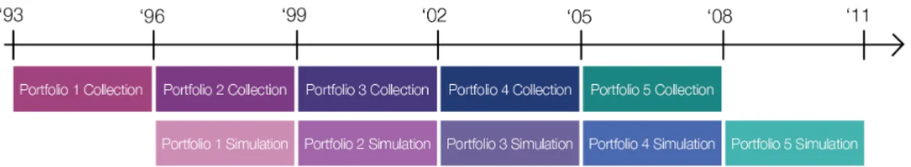
In order to get as unbiased results as possible, the data is divided into 6 time periods. Using several time periods instead of one may minimize the effects of temporary fluctuations in commodity prices that could exist if only one single time period is chosen. Furthermore, we believe that companies aspire to plan for and make forecasts about strategical changes in their product portfolios with shorter intervals than 9 years, which the data would have been divided into if only one sampling period and one testing period were to be used. A portfolio obtained from historical data from one period will be tested on data from the subsequent period; consequently there are 5 periods from which portfolio compositions are collected, and 5 periods on which the portfolios are tested. These are subsequently all ana-lyzed individually. The process is illustrated in Figure 4.1.

(28)

Figure 3.1. Portfolio collection and simulation. The portfolio composition given by historical data from one time period is simulated on data from the subsequent time period.

For every time period, first of all, the daily returns, the standard deviations, the variances and the means of the returns, which are the variables used by Markowitz (1952), Sharpe (1964) and Lintner (1965a, 1965b), are calculated for the commodities. Second, correlation and covariance matrices are constructed using formulas 2.2 and 2.3 in order to find rela-tionships between the different commodities as well as the indices. This is necessary in or-der to be able to calculate the standard deviation of a specific portfolio. Thereafter the tangent portfolio, the minimum risk portfolio and the Black-Litterman portfolio are ob-tained using this data.

The MATLAB code that is used to generate the portfolios is available upon request from the authors.

3.1 Assumptions

The following assumptions are made:

1. Producers cannot use short sales, only speculators

2. Lending and borrowing is both possible at the risk-free rate 3. The expected return is equal to the historical mean return 4. The risk free-rate is the yield of the 3-year U.S. T-bill

5. The production cost of a commodity is equal to its current market price

6. Non-agricultural commodities have no seasonal component

7. The market capitalization factor (𝑤_!"#) is assumed to be redundant.

3.2 Modern Portfolio Theory

The individual assets are plotted with respect to their mean return and their standard devia-tion, in a graph where the X-axis represents the standard deviation and the Y-axis repre-sents the mean return. Thereafter the portfolio with the smallest standard deviation, the minimum risk portfolio, is calculated and plotted in the graph, as well as with the portfolio with the highest mean return. These two portfolios are the ones located at the very far right

(29)

and at the very far left on the efficient frontier. The next step is to draw the efficient fron-tier, which is done by plotting an abundance of efficient portfolios, or corner portfolios as described by Markowitz (1952), between the minimum risk portfolio and the maximum re-turn portfolio. Subsequently, the tangency portfolio, i.e. the most efficient portfolio, needs to be found. This is the portfolio located where the Capital Market Line intersects with the efficient frontier. The CML has an intersect equal to the risk-free rate and its slope is also known as the Sharpe Ratio, obtained by the following formula (Sharpe, 1966):

𝜇_!− 𝜇_!

𝜎_! (3.1)

where

𝜇_! is the mean return of the market portfolio 𝜇_! is the return of the risk-free portfolio

𝜎_! is the standard deviation of returns of the market portfolio

As mentioned above, the tangent portfolio is the portfolio on the efficient frontier that in-tersects with the CML. The slope of the CML, the Sharpe ratio, is maximized on this point. Since 5 time periods are used to find optimized portfolios, a total of 5 tangent portfolios are found. In addition, the compositions of the 5 minimum risk portfolios, one for every time period, are found. These risk-minimizing portfolios are the ones with the lowest standard deviation on the efficient frontier and consequently located at the very left of this line. The future 3-year return, which is the simulation or testing period, is then calculated for every portfolio using the historical daily closing spot prices. For a tangent portfolio with a sampling period from September 1, 1993 to September 1, 1996, the prices from Septem-ber 2, 1996 to SeptemSeptem-ber 2, 1999 is used as the testing period during which the future re-turn as well as the standard deviation, variance and mean are calculated. For a risk-minimizing portfolio with a sampling period from September 1, 2001 to September 1, 2004, the prices from September 2, 2004 to September 2, 2007 is used for the analysis by finding the future return, standard deviation, variance and mean. The total returns as well as the yearly returns, along with the standard deviations and variances of these returns, are then compared to portfolios for every testing period consisting of all the commodities with equal weights. The individual commodities during the same testing periods will also be used for comparison to examine the effects of diversification.

(30)

3.3 Black-Litterman

The Black-Litterman model is a Bayesian approach to asset selection, blending the views generated by quantitative financial models with the views of investors. To maintain an un-biased study the investor views will be modeled using another quantitative model; Geomet-ric Brownian Motion.

3.3.1 Market view

The Implied Equilibrium Return Vector as Π = 𝜆Σ𝑤!"# where 𝑤!"# is a market

capitali-zation weighting scheme, which is used to constrain a portfolio and overcome the prob-lems associated with low market capitalization (Idzorek, 2002). There is no direct counter-part to market capitalization for commodity markets since commodities are held in a varie-ty of ways (Goldman Sachs, 2012; Holthausen and Hughes, 1978). Satchell and Scowcroft (2000) use an equally weighted market capitalization factor. Since there is no equivalent to the market capitalization factor for commodities we will use an equally weighted market capitalization scheme.

Goldman Sachs (2012) states that indices in equity markets are market capitalization weighted. Without a proper index, a scalar value for global risk aversion cannot be deter-mines; therefore in this study we rely on using the risk aversion coefficient as a vector with weights that equal 1. In turn the market capitalization factor becomes a scalar rather than a vector. The new Implied Equilibrium Return Vector remains as written in equation 2.8. The risk aversion coefficient 𝜆 is a 1 x N column vector calculated as in equation 2.9. The equal weighting scheme are in turn calculated as a scalar using 𝑤!" = _!! where 𝑛 is the

number of assets.

As Figure 3.2 illustrates below, the Prior Equilibrium Distribution is normally distributed (𝑁 ~ (Π, 𝜏Σ)) with the Implied Equilibrium Return Vector as a mean. In the article by He and Litterman (1999), they suggest using a 𝜏 of 0.05 or 5%, which is what we will rely on in this study since it is co-authored by one of the original authors of the Black-Litterman pa-per and can therefore be regarded as credible.

(31)

Figure 3.2. The probability distribution of the market view.

3.3.2 Investor Views

Black and Litterman (1992) use well-known investment strategies to generate views that would mimic the investment strategies of actual investors. In order to maintain an unbiased market forecasting view, we rely on quantitative models rather than subjective views. Schwartz and Smith (2000) state that the long-term dynamics of commodity spot prices can be modeled with a Geometric Brownian motion. Schwartz and Smith (2000) state that both spot and futures prices are assumed to follow two distinct processes:

• Long-term dynamics - Assumed to follow a Geometric Brownian motion.

• Short-term fluctuations: Assumed to follow an Ornstein-Uhlenbeck equilibrium-reverting process, set by an equilibrium generated by the long-term Geometric Browni-an motion.

Schwartz and Smith (2000) show that for oil futures prices, the mean-reversion of the Ornstein-Uhlenbeck process converts to its long-term equilibrium after six months. Schumpeter (1939) in his research into business cycles finds that a Kitchin inventory cycle is a three-year business cycle defined as a period of accumulation and deaccumulation of inventory. The time periods used throughout this study is set as three years long, therefore

(32)

short-term fluctuations in the spot commodity prices generated by the stochastic Ornstein-Uhlenbeck process can be disregarded since it is assumed to pan out to its long-term equi-librium. Coincidentally Berck (1981) uses a three-year moving average in his model for pre-dicting the future spot prices of agricultural commodities.

Geman (2005) defines the Geometric Brownian motion as described in formula 2.13 where the volatility (𝜎) factor is assumed to be constant and determined using historical volatility. The drift factor (𝜇) parameter is estimated using historical spot prices. The drift rate is as-sumed to be equivalent to the historical mean daily returns. To maintain unbiased investor views we generate views for all assets rather than just a few. The investor views (𝑄) are therefore set as a 1 x N column vector.

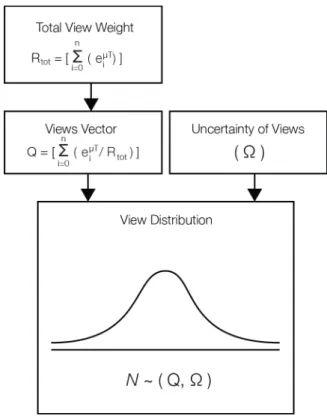
Figure 3.3 illustrates how the views, as generated by Geometric Brownian Motion, are blended with the uncertainty of each view to generate a expected return vector representing the investor views; using the simplification by Hull (2009) that the expected future value is the drift rate continuously compounded until time 𝑇. The range of every individual view, 𝑄_!, is −1 ≥ 𝑄! ≤ 1, with the entire view vector, 𝑄 = 1. The views are calculated so that

the weights of the entire view vector equal 1. Relying on the article of He and Litterman (1999) we use the same values for uncertainty of views (Ω), which is set at 5%.

(33)

3.3.3 Posterior Portfolio

Although the Implied Equilibrium Return Vector Π and the investor views are calculated in a different manner; the posterior combined return vector is calculated in the same way us-ing equation 2.10. The posterior covariance matrix of the tilted portfolio is also calculated in the same way using equation 2.11. The posterior combined return vector and the poste-rior covariance matrix can be used to generate an efficient frontier. However, the weights of the optimal tilt portfolio are generated using equation 2.12 by Walters (2009) rather than obtained using the tangent portfolio set forth by efficient frontier. This is also in line with the article by Black, Jensen and Scholes (1972) where they suggest that relaxation of the ex-istence of risk-free lending and borrowing leads them to generate an equilibrium Capital Asset Pricing Model, which is the foundation of the Black-Litterman formula.

Figure 3.4 shows how the tilted portfolio is generated by blending the quantitative view generated by the market view, with the investor views generated by the Geometric Browni-an motion. Since we assume that producers of commodities cBrowni-annot take short positions in assets, the weights of all assets are constrained so that all non-positive assets are set to a weight of 0 and the entire portfolios’ weight equals 1. To generate the weights for the op-timal tilt portfolio a scalar value for Δ. He and Litterman (1999) assume a Δ equal to 2.5, therefore we have used the same scalar value.

(34)

Figure 3.4. Creation of the tilted portfolio by blending the quantitative market view and the investor views.

3.4 Optimal Portfolio Testing

The first test of the efficient portfolios is done by comparing the future returns and stand-ard deviations on portfolios obtained from Modern Portfolio Theory and the Black Litter-man model. The individual commodities are also used for comparison in order to scruti-nize the validity of the models and the effects of diversification. Subsequently, the portfoli-os obtained from MPT are compared to the ones obtained from the Black Litterman in or-der to find which of the approaches that is the most risk minimizing, which is the portfolio with the lowest standard deviation calculated as the square root of equation 2.1. In addi-tion, it is examined which of the portfolios that optimize returns the most, which is meas-ured by equation 2.5.

(35)

3.5 Application to Existing Mining Companies

The efficient portfolios obtained from Modern Portfolio Theory and the ones given by the Black-Litterman model are then compared to the actual product portfolios of selected min-ing companies. The reason for choosmin-ing minmin-ing companies is because of the fact that his-torical prices for the products mining companies manufacture and sell are available. The mining companies that are used for as comparison are Boliden AB (listed on NASDAQ OMX Stockholm), Lundin Mining AB (listed on the Toronto Stock Exchange), BHP Billi-ton (dual-listed on the Australian Securities Exchange and the London Stock Exchange), Vale S.A. (listed on BM&F Bovespa), Rio Tinto plc. (listed on the London Stock Ex-change) and Xstrata plc. (listed on the London Stock ExEx-change). These companies are all public, which means that their financial statements are available to the public, even though some of these firms do not have reports stretching as far back as 18 years accessible. By looking at the yearly financial reports from these companies, the product portfolios are found. The compositions given by the annual reports are presented according to their re-spective heft; consequently this is converted to a market value weighted portfolio using the metal prices as of the last day of the fiscal year. The testing period will be from 1996 to 2011 and is done so that the mining companies’ actual portfolio composition as for one year is compared with the efficient portfolios obtained using the data from a 3-year period ending the same year. The future performances of these portfolios are then compared, us-ing data from the subsequent 3-year period. Values for mean return, standard deviation and return / risk ratio are compared and then analyzed using equation 2.1 and 2.5. This in order to investigate if the portfolio compositions given by the models provide a better risk mini-mization, measured by the standard deviation, or a higher degree of return optimini-mization, measured by the return / risk ratio than the mining companies’ product portfolio. Fur-thermore, it is examined whether the MPT or the Black-Litterman model is the most ap-propriate approach by comparing the outcomes from the models. Some of the firms may produce other commodities than the 11 that are used in this study; in these cases, those commodities are omitted.