Discrete Event Simulation for Aftermarket Supply Chain

IN

DEGREE PROJECT MECHANICAL ENGINEERING,

SECOND CYCLE, 30 CREDITS ,

STOCKHOLM SWEDEN 2020

Discrete Event Simulation

for Aftermarket Supply Chain

JAGATHISHVAR JAYAKUMAR

LAURA ALBORS MARQUÉS

KTH ROYAL INSTITUTE OF TECHNOLOGY

Discrete Event Simulation for Aftermarket Supply Chain

JAGATHISHVAR JAYAKUMAR

LAURA ALBORS MARQUÉS

KTH Supervisor: Jerzy Mikler

Volvo Supervisors: Joakim Andersson and Niklas Samuelsson

KTH Examiner: Daniel Tesfamariam Semere

© LAURA ALBORS MARQUÉS, JAGATHISHVAR JAYAKUMAR, 2020.

Department of Production Engineering and Management

School of Industrial Engineering and Management

KTH ROYAL INSTITUTE OF TECHNOLOGY

Stockholm, Sweden 2020

i

ABSTRACT

Planning of an Aftermarket Supply Chain is a very complex task. This is due to an unpredictable demand driven by the need for maintenance and repair. This drive translates to a high variety of lead times, a large number of stock-keeping units (SKUs) and promise to deliver spare parts during its full lifecycle. With all these complexities in place, optimizing and parametrizing the planning process is a difficult and time-consuming task. Moreover, the current optimization tool focuses only on one node (each warehouse individually) of the whole Supply Chain, without considering the information such as inventory levels of the other nodes. Hence, the Supply Chain is not completely connected, making it difficult to get a better understanding of the system performance to identify cost draining areas. This leads to capital being tied up in the upstream of the Supply Chain and later adding unnecessary costs like high inventory costs, rush freight costs, return or scrapping cost.

In this study, Discrete Event Simulation (DES) is explored as an additional optimization tool that could analyse and improve the performance of the whole Supply Chain. To do that, the functioning of a node is modelled by replicating the logics behind the flow of material, which includes analysing some manual workflows which are currently present. In addition, the information needed from the orders, order lines and parts are mapped. The later part of the study aims to connect all the nodes to form a whole overview of the Supply Chain and further perform optimizations globally.

As an outcome, Multi-Echelon Inventory Optimization has been performed on the whole Supply Chain connecting all the nodes and thus getting an overview. Furthermore, the impact of different parameters has been studied on the whole model to understand the sensitivity of parameters such as variations in lead time and demand. Finally, different what-if scenarios such as COVID-19 and problems with delay in suppliers were studied, which could help understand the impact of unforeseen situations are analyzed.

KEYWORDS:

Aftermarket, Demand Planning, Discrete Event Simulation, Multi-Echelon Inventory Optimization, Supply Chain, Digital Supply Chain

ii

SAMMANFATTNING

Planeringen av en eftermarknadskedja är en mycket komplex uppgift. Detta beror på en oförutsägbar efterfrågan som drivs av behovet av underhåll och reparation. Enheten översätter till många olika ledtider, ett stort antal lagerhållningsenheter (SKU) och kapacitet att leverera reservdelar under hela dess livscykel. Med alla dessa komplexiteter på plats är optimering och parametrering av planeringsprocessen en svår och tidskrävande uppgift. Dessutom fokuserar det nuvarande optimeringsverktyget bara på en nod (varje lager separat) i hela leveranskedjan utan att beakta informationen som lagernivåerna för de andra noderna. Därför är försörjningskedjan inte helt ansluten, vilket gör det svårt att få en bättre förståelse för systemets prestanda för att identifiera kostnadsavtappningsområden. Detta leder till att kapital binds i den övre strömmen i försörjningskedjan och senare lägger till onödiga kostnader som höga lagerkostnader, snabba fraktkostnader, retur- eller skrotningskostnader.

I denna studie undersöks Discrete Event Simulation (DES) som ett ytterligare optimeringsverktyg som kan analysera och förbättra prestanda för hela försörjningskedjan. För att göra det modelleras en nods funktion genom att replikera logiken bakom materialflödet, vilket inkluderar analys av några manuella arbetsflöden som för närvarande finns. Dessutom kartläggs all information som behövs från beställningar, orderrader och delar. Den senare delen av studien syftar till att ansluta alla noder för att bilda en hel översikt över försörjningskedjan och ytterligare utföra optimeringar globalt.

Som ett resultat har Multi-Echelon Lageroptimering utförts i hela försörjningskedjan efter att alla noder har anslutits och därmed fått en översikt. Dessutom har effekterna av olika parametrar studerats på hela modellen för att förstå känsligheten hos parametrar som variationer i ledtid och efterfrågan. Slutligen studerades olika tänkbara scenarier som COVID och problem med förseningar hos leverantörer, vilket kan hjälpa till att förstå effekterna av oförutsedda situationer.

NYCKELORD:

Aftermarket, Demand Planning, Discrete Event Simulation, Multi-Echelon Inventory Optimization, Supply Chain, Digital Supply Chain

iii

ACKNOWLEDGEMENTS

First, we would like to thank our supervisors at Volvo, Joakim Andersson and Niklas Samuelsson. Their support and feedback guided us throughout the thesis. Their involvement and experience even through the COVID-19 Pandemic has helped us to get a better understanding of Volvo’s Aftermarket Supply Chain and encouraged us towards the thesis’ goal. We would also like to thank all the involved people at Volvo, especially in Service Market Logistics, for their time and help to get the right information we needed. Their enthusiasm in the project motivated us to work harder and get things done.

We would also like to thank our supervisor at KTH, Jerzy Mikler. His time and experience guided us through building the model. His interest in our questions and findings drove us to get a more detailed and understandable model.

iv

NOMENCLATURE

ABBREVIATIONS

SKU: Stock Keeping Units DES: Discrete Event Simulation IP: Inventory Position

OL: Order Level

TSL: Target Service Level

OEM: Original Equipment Manufacturer IMS: Inventory Management System

MEIO – Multi-Echelon Inventory Optimization VCE: Volvo Construction Equipment

DIM: Dealer Inventory Management DIP: Dealer Inventory Planning CDC: Central Distribution Centre RDC: Regional Distribution Centre

v

CONTENTS

Chapter 2 –Theoretical Framework ... 5

2.1. Aftermarket Supply Chain ... 5

2.2. Inventory Management ... 6

2.3. Discrete Event Simulation ... 7

2.4. Discrete Event Simulation in Supply Chain ... 8

2.5. Modelling Stochastic Variables ... 8

2.6. Case Studies using Simulation ... 9

Chapter 3 – Methodology or Model Specification ...10

3.1. Research Design ...10

3.2. Research Quality ...11

3.3. Modelling the Supply Chain ...11

3.4. Material Flow Component ...12

3.5. Control System ...16

3.6. Performance Measurement or KPIs ...19

3.7. Data Management ...20

3.8. Modelling MEIO using DES ...21

3.9. Sensitivity Analysis and Scenario Comparison ...21

Chapter 4 – Quantitative Analysis ...22

4.1. Validation ...22

4.2. MEIO Implementation ...24

4.3. Sensitivity Analysis ...25

4.4. What-if Scenarios ...26

Chapter 5 – Implementation Plan ...28

5.1. Expansion of the model ...28

5.2. Workflow ...28

vi

6.1. Research Finding ...30

6.2. Future Work ...31

References ...32

Appendices ...35

Appendix 1. Relationship between parameters ...35

vii

List of Figures

Figure 1. Volvo's Supply Chain Design. ... 3

Figure 2. Decision players in the Aftermarket Supply Chain. ... 3

Figure 3. Classification of the issues from Strategical to Operational. ... Error! Bookmark not defined. Figure 4. Inventory levels in the SC. ... Error! Bookmark not defined. Figure 6. The components of a node... 11

Figure 7. Ordering flow in a node. ... 12

Figure 8. Refilling Logic – Decision Tree for Normal and Rush Orders ... 12

Figure 9. Order Classifications based on constraints. ... 13

Figure 10. Parameters which define the Order Level and Order Quantity. ... 16

Figure 11. Comparison of the forecast and demand in MMI system and model for one part. ... 22

Figure 12. Comparison Order Level Calculations. ... 23

Figure 13. Costs for the different optimizations in the Supply Chain. ... 25

Figure 14. Costs for the different scenarios. ... 27

Figure 15. Workflow Structure. ... 28

Figure A 1. Study of the CDC costs when varying TSL in CDC. ... 35

Figure A 2. Study of the system when varying the demand distribution. ... 36

Figure A 3. Study of the system when varying LT in RDC. ... 36

Figure A 4. Study of the system when varying LT in CDC. ... 37

Figure A 5. Study of the system when varying the daily demand. ... 37

Figure A 6. Nodes and flow of material between them in the model. ... 38

viii

List of Tables

Table 1. Costs Comparison: MMI and DES, for one part. ... 23

Table 2. Results for the minimization of costs. ... 24

Table 3. Results for the maximization of service level. ... 25

Table 4. Results for the COVID19 scenario. ... 26

1

Chapter 1 – Introduction

In this chapter, the background of the study is presented both from a theoretical and company perspective. The

existing problem which translates to the problem statement is explained. Following is the formulation to the aim

of this study. Later the delimitations of performing this from a practical view is described.

1.1. Theoretical Background

Supply Chain consists of all the activities involved in satisfying a customer’s request. These activities encompass right from sourcing of raw materials to manufacturing goods and finally delivering to customers (Chopra and Meindl, 2016). The pursuit for competitiveness advantage has driven Original Equipment Manufacturers (OEMs) to not only focus on bringing new products to the market but also focus on servicing of sold products. This has led to two classifications within the Supply Chain based on what commodity is delivered: i) Manufacturing Supply Chain and ii) Aftermarket Supply Chain (Sengupta, Heiser and Cook, 2006). The Manufacturing Supply Chain, which is the traditional Supply Chain, focuses on delivering new products to customers whereas, the Aftermarket Supply Chain focuses on maintenance/repair of existing products.

Realizing the potential within the Aftermarket Supply Chain, OEMs have started focusing on establishing and continuously developing the same (Theodore Farris, Wittmann and Hasty, 2005). This is nowadays contributing to nearly 50% or even more of the revenue for some of the OEMs (Cohen and Agrawal, 2008). Moreover, studies prove that this is directly related to an increase in customer loyalty which could later influence their decision when buying new products (Cohen and Agrawal, 2008).

Even though the opportunities look very appealing, the Aftermarket Supply Chain is very complicated as there are lot uncertainties involved compared to the Manufacturing Supply Chain (Andersson and Jonsson, 2018). For example, there could be similar characteristics between these two types of the Supply Chain such as a unique demand driver or a demand pattern or a Supply Chain network design (For et al., 2019).

However, the factors influencing these characteristics are entirely different. One such characteristic is the demand driver that depends on a customer’s need for a new product, for a Manufacturing Supply Chain. On the other hand, it depends on the need for maintenance or repair of an existing product in the Aftermarket Supply Chain. New approaches within Manufacturing Supply Chain such as “make to stock” or “engineer to order” have led to reduced stock-keeping units (SKUs) (Olhager and I. Prajogo, 2012). However, this is not the case in an Aftermarket Supply Chain, as the SKUs are nearly 10-100 times of the actual demand leading to large sums of capital tied up. Even though there is huge potential within the Aftermarket Supply Chain, it could present difficulties when planning the same.

A lot of research has been carried out over the years to address the issue of reducing the high SKUs in the Aftermarket Supply Chain. Especially by focusing on improving the Inventory Management System (Tako and Robinson, 2012). Various research focusing on different areas independently or on the whole system is being explored constantly. This has led to the application of Machine Learning (Carbonneau, Laframboise and Vahidov, 2008), Big Data Analytics (Andersson and Jonsson, 2018; Tiwari, Wee and Daryanto, 2018), and Information Sharing (Hall and Saygin, 2012) on Inventory Management Systems.

2

There has been a constant addition of technology to improve the performance of the Inventory Management System. However, a hurdle in the Inventory Management System is that the basics of the system is based on the classical analytical model or mathematical model. The analytical model generally consists of simple equations to define the inventory levels based on the demand that flows towards the warehouse. This approach leads to an optimal setting for a warehouse individually and the effect of this is the local minima or local inventory optimizations (Riddalls, Bennett and Tipi, 2000). The local minima will

not be an optimal solution as in the real world, as optimizing one warehouse could influence other warehouses. Understanding the consequence of the local minima, efforts have been made to develop complex analytical models to find global minima or the Multi-Echelon Inventory Optimization (MEIO). Clark-Scarf and Metric are two famous analytical approaches that could perform MEIO by considering the neighbouring warehouse in the Supply Chain. Axsäter gives a summary of both these approaches (Axsäter, 2015). However, these approaches were too complex to implement. Dominguez(Dominguez, Framinan and Cannella, 2014) suggests a contradiction that an analytical model could not be used to solve

the dynamics, stochastics and uncertainties problems, given their complexity and non-linearity. Instead, this problem could be easily solved using a simulation with an optimizing algorithm. As the optimizing algorithm only needs an objective, some constraints and input variables. The output will be a global minimum; however, the immaturity of simulation environments previously prevented their implementation in industrial solutions.

Recent Advancements in simulation environments and versatility in its applications has enabled the use of simulations like Discrete Event Simulation (DES), Continuous Event Simulation, Agent-Based Simulation and Dynamic Systems in various industries(Banks, 1998). Moreover, these simulation models have the potential to act as decision support systems by visualizing the complexity and modelling the uncertainties which are not feasible in analytical models. Thus, forming the basis for a digital platform for Supply Chain that can act as a testbed for developing and testing new technology and further helping in understanding the dynamics involved. Simulations also help in releasing the full potential of other technologies discussed earlier.

DES, in particular, has been gaining attention due to its versatility and simplicity in solving various Supply Chain issues (Tako and Robinson, 2012). Banks(Banks, 1998) explains in details the vast applications with examples which contribute to its continuous platform development and its ability to be combined with other platforms to form hybrids models which make them an interesting simulation environment.

1.2. Company Background

Volvo Group AB, from here on termed as Volvo is an iconic symbol of Sweden and known throughout the world as a leader of manufacturing trucks, buses, construction equipment, marine and industrial engines. Volvo has segregated all its production and logistics operations into a separate organization called the Group Truck Operations, under which comes the Service Market Logistics department. The Service Market Logistics department manages the Aftermarket Supply Chain ensuring that Volvo’s sold products keep the optimal uptime with no unplanned stops, with the lowest possible operating costs.

The setup of Volvo’s Aftermarket Supply Chain structure is a divergent system that can be referred to a tree-like structure as shown in Figure 1, where the warehouse is supplied only by its immediate successor.

A Central Distribution Centre (CDC) acts as a sourcing point from an external supplier and distributes goods to the Regional Distribution Centre (RDC) in key areas throughout the globe. These RDCs supply the Dealers which come under its region to satisfy all Volvo customers. This setup could also be expressed as a 3 Level Echelon structure as shown on the left side of Figure 1.

3

Owing to a large Aftermarket Supply Chain network with thousands of warehouses throughout the globe. Volvo has classified its human resources into different team’s majority based on the duties. An Analyst Team that optimizes the performance of the warehouses individually by finding the right balance between the costs and customer service level that is the local minima. The Operation Team ensures the correct functioning of the warehouses based on the settings set by the analysts. This is done by ensuring that the orders are placed or recovering any orders that have not been sent. The analyst team who handle the CDCs and RDCs are called Dealer Inventory Planning (DIP) and the ones who handle the dealers are called Dealer Inventory Management (DIM) Team. The Operations Team who are responsible for the CDCs are called the Material Planners and the ones responsible for the RDCs are called Refillers. As shown in Figure 2, each team is responsible for specific warehouse and operations within the Aftermarket Supply Chain.

The dealers handle their operations locally, Volvo has no governance over them.

1.3. Problem Statement

As it was seen in Section 1.1, over the years the current analytical model has led to obtaining a different

local minimum for each warehouse. This approach has ignored the consequences of local optimization on the neighbouring warehouses. To improve the current scenario, it is necessary to get an overview of the whole Supply Chain by exploring MEIO instead of local optimization.

Previously, Volvo carried out a study in collaboration with Syncron AB, to explore the use of the METRIC approach to implement MEIO. This study was conducted on a particular brand within Volvo Group - Volvo Construction Equipment and focused only on the two levels of echelons, which encompasses only

Figure 1. Volvo's Supply Chain Structure.

4

one RDC and the dealers within its region. This project concluded with some important findings that the obtained customer service level was increased while reducing the cost when an MEIO of the Supply Chain was introduced. On the other hand, the demerit was that the hindrance of expansion of the model to the whole Supply Chain which coincides with the theoretical background (Dominguez, Framinan and Cannella, 2014).

The learning from the previous study has led Volvo to explore the use of simulation models, especially DES for solving not only the MEIO problem but also understanding the dynamics involved which is not possible with analytical models. To perform this study a similar approach to the previous study opted, where all three levels of the echelon within the Supply Chain were considered.

1.4. Aim

The problem statement lays the foundation for the initial aim of this thesis, that is to test the feasibility of using Discrete Event Simulation for Volvo’s Aftermarket Supply Chain. This forms the basis of the first research question:

RQ1: How can the Aftermarket Supply Chain be modelled using a DES?

To answer RQ1, a bottom-up approach to building a simulation model of the current Inventory Management System has been performed. Once the model is developed, it is compared with the actual Inventory Management System to see how Volvo’ Aftermarket Supply Chain performs with MEIO. Thus, the second research question is as follows:

RQ2: How effective is the Multi-Echelon Inventory Optimization for proceeding with a DES model?

After comparing the effectiveness of MEIO, a study about other benefits of using the model have been carried out. This has been done by analysing the influence of the parameters in the final objectives. Thus, formulating the last research question:

RQ3. What are the main parameters influencing inventory optimization?

1.5. Delimitations

First of all, the scope has been narrowed down to be able to create a model with a good representation of the Supply Chain, modelling it in the limited time of the thesis project. The model is created only for one of Volvo’s brands, Volvo Construction Equipment.

Secondly, data reliability is another limitation, as not all aspects of the Supply Chain are managed by Volvo. Some data are not reliable or sometimes it could not be available. Moreover, as some of the data is missing, it would be difficult to compare the reliability of the model.

Thirdly, Volvo has quite an automated Supply Chain, meaning that most of the calculations and decisions are automated. However, there are some exceptions in which the decisions are made manually. These decisions are hard to model and simulate in a discrete event simulation model. Due to this, not all logics can be thoroughly represented.

Lastly, the COVID 19 situation has introduced new limitations to the thesis. The company had been affected and as a consequence, people were laid off for 10 weeks. This period corresponds to half the period of the thesis. The situation has impacted communication, complicating information gathering. Moreover, assumptions had to be that were initially not planned.

5

Chapter 2 –Theoretical Framework

In this chapter, an overview of the Aftermarket Supply Chain has been presented, followed by a focus on Inventory

Management. After that, the framework of the current inventory management system has been elaborated along

with its limitations. Following is the description of what is Multi-Echelon Inventory Optimization and its benefits.

The second section of this chapter focuses on Discrete Event Simulation, its ability to solve Multi-Echelon Inventory

Management, along with a brief discussion of how DES could be used to solve other issues in the Aftermarket

Supply Chain. Later, the consideration when developing a DES model is also elaborated. Finally, some previous

case studies have explained, which lay the foundation for the model to be built on.

2.1. Aftermarket Supply Chain

Understanding the Aftermarket Supply Chain better in practical terms could be done by expressing its objective and its associated different decision levels. The objective is to maintain a high service level, which is the percentage of orders delivered to orders received while reducing the costs incurred (Axsäter, 2015). The decision levels involved in the Aftermarket Supply Chain have been classified on a high level into three categories: strategical, tactical and operational (Chopra and Meindl, 2016). These levels are categorised based on the frequency of actions needed to be taken and the time horizon of the impact of the decisions. Strategical level decisions are the broad level decisions such as planning a Supply Chain configuration, the capacities of the warehouse, the location of the warehouse and the modes of transport between the warehouses. Similarly, some of the tactical level decision involves planning the forecast for the month and adaptations to prices of SKUs. Finally, the operational level involves daily decisions such as handling individual customer order, handling pickups and setting delivery schedules (Lee et al., 2002).

6

Tako (Tako and Robinson, 2012) further expanded this high-level classification elaborating the issues ranging from strategical to tactical to operational level as shown in Figure 3. This elaboration gives a

detailed scale of how the different decisions are taken. Starting at the top are purely strategical level decisions, moving down the scale gives an increased tactical decision level involved while reducing the strategical level decisions. Similarly, when moving from tactical to the operational level.

2.2.

Inventory Management

Complexities arise when handling many parts, especially for Volvo, as the stocked parts are around 700,000 parts. The ideal way to find an optimal order-level and order quantity would be to understand the pattern of demand and define a suitable forecasting and order-level calculation method to set the upcoming month’s forecast, order-level, and order quantity. However, unique calculations are not practical as its resource-intensive approach and this is where Inventory Management plays an important role, to have an organized structure to manage all the parts. The standard common way to control the order-level is done by grouping the parts based on ABC Classifications keeping Pareto Rule in mind, which is 20% of parts contribute to 80% of the revenue. More weights in the form of inventory policies are allocated to the parts that contribute to the major of the revenue.

Although all the decision level in the spectrum needs to be optimized to get an efficient Supply Chain as shown in Figure 3. There has been a lot of focus on inventory management specifically, as it involves both

tactical and operational level decision (Ivanov, 2010). Moreover, the influence of the decisions taken at inventory management level is quite broad starting from the lowest level issue in the spectrum up to bullwhip effect, as shown in Figure 3. The structure of Volvo’s Supply Chain explained under Section 1.2

further justifies the involvement from the two different decision levels. This involvement could be elaborated from a practical point of view of how Volvo works with its Supply Chain.

From a tactical perspective, it includes all the activities which concern the performance optimization in a warehouse, which could be related to the role of the Analysts Team in Volvo’s Supply Chain. This refers mainly to the configuring of what the reorder level is, referred to as order-level hereafter, and defining an economic order quantity, referred to as order quantity hereafter. This tactical level decision is reviewed periodically, it is done monthly in Volvo’s system, based on the previous month’s demand.

On the operations perspective, it includes all the activities which concern the material flow and could be related to the Operations Team. The main activities involved are ordering and delivering. Ordering refers to the act of defining an order size which is multiple of the order quantity generated when the current order level is below the set Inventory Position. Delivering refers to supplying the parts to customers. The traditional analytical model approach in inventory management is by finding a local minimum of order-level and order quantity for a part in a particular warehouse based on its demand data. The outcome

7

of this system is that the inventory levels are low in the dealers but high in the upper echelons as shown on the left in Figure 4. The limitations are that the inventory costs are high, and the system is not able to

deliver parts to the customers. This has led to the seek for global minima which could potentially reduce inventory level in the upper echelons and on the contrary increase the service levels at the lower echelons.

2.2.1.

Multi-Echelon Inventory Optimization

The concept of Multi-Echelon Inventory Optimization (MEIO) is simple, that is defining a feasible order-level and order quantity by considering the same in all the warehouses the part exists (Grob, 2018). The outcome of MEIO consists of reducing the inventory level throughout the Supply Chain. The amount of unnecessary inventory in the first and second echelon are reduced, optimizing the total stock level (De et

al., 2020), as shown on the right in Figure 4. Simultaneously, high availability is ensured in the network and

customer's demands are met. This concept leads to having a material flow only when a customer places an order, avoiding the Bullwhip Effect (Padmanabhan, 1997). The consequence of this could be reducing the flexibility in the upper echelons of the Supply Chain (Axsäter, 2015). However, this does not possess any risk as the availability of SKUs in the lower echelon are higher reducing backorders that are generated based on local minima.

The major approaches to implement MEIO are through analytical models, or Operational Research techniques or Simulations models. The analytical model such as METRIC (Sherbrooke, 1968) or Clark-Scarf’s methods (Clark and Scarf, 1960) uses a complex equation to model the order-level. Hence, the analytical models are complex to build and a lot of approximations must be considered, therefore there are not many implementations and still mostly in the research phase. Operation Research techniques like linear programming, queuing theory, Markov chain and dynamic programming can be used, however, they don’t consider the system dynamics perspective (Riddalls, Bennett and Tipi, 2000). Use of simulations was generally not seen as an option as it always considered to be underdeveloped technology that was not up to industry standards. However recent developments of robust simulations environment have provoked various industries to use simulations for different studies. Similarly, the approach of obtaining MEIO through simulation has been attempted and has proved very beneficial (Kleijnen, 2014).

2.3.

Discrete Event Simulation

Discrete event simulation (DES) is a tool used to model real-world systems as a sequence of events that change over time (Fishman, 2001). DES environment is built by abstract modelling where only the necessary features with precedence and mathematical relationships between the events are considered. This approach of DES models where changes occur only when there is a trigger by an event makes it less computationally intensive and diverse for various applications. ExtendSIM 9 is the DES software used in this thesis to build the model.

The architecture of ExtendSim like any other DES model is a collection of several elements in an organized manner (Banks, 1998) and some of these elements are as follows, but not limited to:

• _{Variables: are a collection of information that is used to define the state of the system at a given} time. Example, the on-hand inventory at any time during the simulation.

• Entity: is a dynamic object that moves through the system triggering changes. Example, the part. • _{Attribute: is the local variables which define properties of an entity. Example, details such as part}

number.

• Activity or Delay: is a known time period that could influence the flow of entities. Example, the delay in flow of entity due to lead time.

8

• Queue: is the arrangement of entity based on an entity’s attribute. Queue is used as a buffer to store and release entities based on rules such as first in first out.

2.4.

Discrete Event Simulation in Supply Chain

The exploration of various simulation environments such as DES, continuous event simulation, agent-based simulation and system dynamics in Supply Chain context has evolved over the years (Lee et al., 2002;

Schieritz and Größler, 2003; Behdani, 2012; Al-fedhly and Folley, 2020). DES models, in particular, have been of keen interest due to their simplicity and versatility. Previously, DES was considered as a black box, due to the lack of a common descriptive language and theoretical framework (Riddalls, Bennett and Tipi, 2000). These issue has been addressed in simulation platforms such as ExtendSim or Anylogic, that are based on C++ and Java respectively. Modelling the right amount of details has been leading DES models to act as decision support systems at all decision levels of Supply Chain. The level of details for the respective decision levels has been compared by Lee (Lee et al., 2002). Moreover, integrating with other

simulation environments can address issues that were not known before (Ingalls, 1998).

The DES based MEIO is done by feeding in parameters to an optimizer with some constraints. The optimizer is based on a common optimization algorithm. In this case of application, the input parameters are the inventory policies, the objective function is to minimize the cost of the whole Supply Chain while the constraint is to maintain a fixed target service level set for the whole Supply Chain. ExtendSIM gives access to the source code which makes it easier to customize the platform for specific applications. The inbuilt optimizer used in ExtendSIM, which like any general optimizer algorithm tries to find the best solution for a problem (Diamond et al., 2007). The optimization algorithm used in ExtendSIM is a

population-based meta-heuristic approach that is called the evolutionary algorithm. Diamond (Diamond, 2003)explains in detail how the algorithm works in ExtendSIM.

There are also other benefits to DES models which unlike any other analytical approaches does not have approximations that needs to be done. On the other hand, DES has more precise calculations based on the detail level of the model which is generally more accurate to any analytical approaches. This also provides an opportunity to do detailed studies like sensitivity analysis and what-if scenario comparisons. Sensitivity analysis helps understand how any parameter’s influence the final objectives of the Supply Chain that is the cost and service level. This is performed systematically using a design of experiment approach. The what-if Scenario is the approach of developing different configuration of the model to study the influence of the parameters.

2.5.

Modelling Stochastic Variables Demand Distribution

DES can model the stochastic nature of a Supply Chain which was not possible in an analytical approach (Lee, Cho and Kim, 2002). Two variables that could be modelled are the demand distribution and lead time. There have been different methods of modelling demand distribution based on previous studies. Syntetos (Syntetos, Babai and Altay, 2012) suggest using the Poisson distribution for all demand points, with a constant mean in which the variance-to-mean ratio for a particular item tends to increase as the period of observation lengthens. However, this approach is applicable only during the earlier phase, but it tends to change into binomial distribution as the time progress and when more data is available (Taylor, 1961). The major influence here is the lifecycle the part, if the part is just been introduced into the market or if it is in its prime phase, or declining phase or the final phase of its lifecycle.

Another approach is using default distribution based on the demand pattern, which is the normal distribution for fast-moving parts, Poisson distribution for slow-moving parts and negative binomial

9

distribution for lumpy-moving parts. This could be more accurate based compared to the previously suggested method and also agree with the order level calculations. However, there are other influences on the demand but they are too complex to model them. Rezaee (Rezaee et al., 2017) states that a simplified

version could be modelled using these apt distributions but not applicable as it leads to a lot of correction factors being introduced and loss of uniqueness based on demand points. These losses could be related to Volvo’s current situation as there are Operations Team just focusing on recovering backorders and constantly re-evaluating the forecast.

Modelling using robust stochastic demand by histograms is another approach which uses a goodness of test to define a type of distribution with parameters based on part’s historical data (Schmitt and Singh, 2009). The benefit is that the demand distribution ambiguity is addressed in this approach and is based on the Chi-squared test. Considering the benefits of this approach, this has been opted to perform in this study. This approach could help define a more accurate order-level if the same distribution is used in its calculations later on.

Lead time is another variable that is an important influential on the objectives of the Supply Chain. Modelling an accurate distribution could be more complex compared to demand as there could a lot of factors influencing it. Ching (Liao and Shyu, 1991) suggests using a normal distribution, however, a similar approach to demand distribution modelling has been used here that could be more accurate (Schmitt and Singh, 2009).

2.6.

Case Studies using Simulation

One of the biggest tech giants, Microsoft along with Goldratt Research Laboratory has developed a

self-configurable simulation model that could implement MEIO. As an outcome, the developed model was able to implement MEIO by using the inbuilt optimizer and a platform to perform sensitivity analysis and what-if scenarios. The model has been acting as a testbed to develop and test new improvements in a safe environment. Microsoft was able to save quarter billion dollars on inventory and hundreds of millions in

scrapping. Furthermore, led to solving four major issues in the Supply Chain: lesser shortages, lesser scraping of products, more revenue and lower inventory (Anylogic, 2020). This case has laid out how the optimization approach could be done in the model to result in real-time savings.

Another case study shows how Eldorado benefitted by using a simulation model as a decision support

system to address issues right from operational, to tactical and finally to strategical level. Moreover, the implementation cost was paid off during the first two months of the implementation. This shows the flexibility of simulation, which has been planned to deal with by introducing modularity in the model (Anylogic, 2020).

Another case is Diageo, which used simulation to not only perform Inventory Optimization but also embed logistics optimization model by including details of transportation costs like border crossing cost, waiting costs in transport, etc. This improved the forecasting accuracy by 20% and reduced SKUs by 40% and logistics cost per unit by 7% (Ivanov, 2018; Anylogic, 2020).

Even if many more case studies can be researched, the previous ones have laid out enough constraints to consider when building the model. Flexibility and modularity are a high priority to ensure the model is future proof and that it can be used to solve strategical level issues in the Supply Chain. A high level of details is required to ensure that other operational level issues like Distribution and Transportation Level can be studied later (Ingalls, 1998).

10

Chapter 3 – Methodology or Model

Specification

This chapter justifies and supports the different decisions taken within the thesis project. This justification is done

by the theoretical resources introduced in the literature review. It introduces the basic concepts needed for

understanding the goal of the project as Supply Chain or Inventory Management. Also, previous studies are reviewed

for comparing them with the new study that this project thesis implied and support the choices.

3.1. Research Design

As the aim of the project revolves around a deductive study, that is testing of a theory for a specific application. The research methodology selected is a quantitative approach based on the definition given by Bryman (Bryman and Bell, 2015). As Volvo’s Aftermarket Supply Chain is complex and enormous with thousands of warehouses, a simplified research process has been selected. The major process involved conducting semi-structured interviews to understand the detailed role of the analysts' team and operations team at different echelon levels. Following is the modelling process which needs to resemble the current process as close as possible. Here the modelling process and interview process was carried on a closed-loop until the model was validated. Once the model validated the final phase of studies occurred that was analysing the model further.

To answer the RQ1, “How can the Aftermarket Supply Chain be modelled using a DES to reduce the total cost?”, the

flow of a single past throughout the whole Supply Chain is mapped. This approach gives an understanding of a simplified version of the Aftermarket Supply Chain and enables the future expansion by replicating the process with other parts. The item selected is sourced from the supplier to the CDC in Gent, then supplied to the RDC in Singapore which covers 13 dealers within its region. The level of details intended to be represented in the model are very detailed including distribution planning.

As the focus is on a high detailed model, there have been complications involved in representing the manual process involved in the operational level. These complications are either simplified or omitted. Each of the simplification or omission has been described in detail in the later section when performed. The answer the first RQ.1 is done by a convergent validation process, where the current inventory management of Volvo has been compared to the performance of the DES model.

Once the model was proven to be validated, the next phase of the thesis was to answer RQ2: “How effective is Multi-Echelon Inventory Optimization using DES model?”. Comparisons of the objective of the Supply Chain

before and after using the DES model for MEIO were performed. To perform this, the DES model was simulated using the historical data of the year 2019 for the assumed part.

Once the results were compared, the next phase of the study was to understand how the parameters influence the objectives of the Supply Chain. Thus the final research question, RQ3: “What are the main parameters influencing the inventory optimization?” This question was answered by developing a sensitivity

analysis model to understand the influence of parameters on the objective of the Supply Chain. Moreover, different what-if scenarios were created to understand how the parameters react to the varying

11

configuration of the model. This was done by convergent validation process done with a comparison of the results obtained through RQ2.

3.2.

Research Quality

The quality of the study, especially in a simulation model involves three steps: verification, validation and reliability of the model. The goal is to create an accurate and reliable model that servers its purpose. The phase of the study can be conducted once the basic specifications have been introduced and the development of the model has been completed (Sargent, 2010).

First, the model is verified, corroborating that it is running without any errors. During this process, the model is debugged to ensure that all the parts of the model work. This can be tested by building the model in different stages and simulating each of them. To do this, the model should be run and checked each time a new logic/flow is included. Another way of verifying the model is by simplifying it and running a simple scenario whose results are expected, reductio-ad-absurdum (Diamond et al., 2007).

Secondly, the model is validated. In the validation, the accuracy of the model is tested, how accurate the model is when representing the real system. A model is considered valid when it is accurate based on the model’s intended purpose, it does not need to replicate every aspect. One of the ways of validating the model is comparing its results of the value of the key parameter indicators with reality, using historical data. Because of that, it is very important to start modelling the current scenario before introducing any improvement or optimization. Some of the parameters that could be compared for validating the model are the total cost, the inventory level in each month and the service level.

Finally, the reliability of the model needs to be studied. For that, the probability of the system to fail should be analysed. Also, how predictable, and detectable that failure is. For establishing high reliable systems, the principles of redundancy, diversity and physical and electrical separation are used as preventive measures against random and common mode failures (Singh and Billinton, 1977).

3.3.

Modelling the Supply Chain

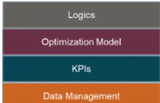
A virtual model of a warehouse is called as a "node" mimicking both its functions and behaviour. A node has been designed such that it comprises of four components: i) Material Flow, ii) Control System, iii) KPIs Monitor and iv) Data Management, as shown in Figure 5. The material flow component consists of

all the logics that are related to the physical flow of goods in a warehouse, which are all the operational

processes. Control System governs how the goods can flow in a cost-efficient way on a monthly basis which are all the tactical processes. KPIs monitor the performance of the node by monitoring the objectives. Data management component manages data needed for the previous components to function. Three different types of nodes have been modelled based on where the warehouse belongs in the echelon level in the Supply Chain. The different nodes are CDC, RDC and dealer. The major difference between the nodes is within the material flow component. The following sections contain the elaboration for each

12

component in a node and also the adaptations that have been done within each component for the different types of nodes.

3.4.

Material Flow Component

This component is the mimic of the ordering system that defines when to order (order-level) and how much to order (order size). In a simulation version, this could be translated to logics defining the flow of material

inwards and outwards a node, called refill and order lines respectively as shown in Figure 6. There are also

minor logics within each of the major logics such as how the material overstock should be treated: scrap and return logics from a refill perspective. Minor logic within order lines is the backorders, which are orders that not being able to be delivered when requested due to no stock. After some time, the backorder becomes a lost sale, due to customer unsatisfaction. The major logics along with their respective minor logics are explained below.

3.4.1.

Refilling Logic

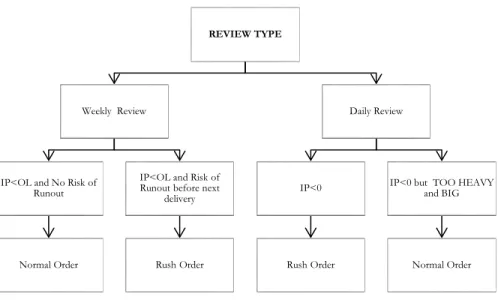
Figure 7. Refilling Logic – Decision Tree for Normal and Rush Orders

Refilling the warehouse is done by only its immediate upstream node. Volvo follows a weekly periodic review policy. During the review, the current Inventory Position (IP) is compared with the set order-level

REVIEW TYPE

Weekly Review

General Condition: IP<OL

Normal Order

Risk of Run Out before next delivery

Rush Order

Figure 6. Ordering flow in a node.

Node

13

(OL) and an order is generated with two defined attributes: order size and order type. The general equation for an Order Size is:

𝑂𝑂𝑂𝑂𝑂𝑂𝑂𝑂𝑂𝑂 𝑆𝑆𝑆𝑆𝑆𝑆𝑂𝑂 = 𝑂𝑂𝑂𝑂𝑂𝑂𝑂𝑂𝑂𝑂 𝐿𝐿𝑂𝑂𝐿𝐿𝑂𝑂𝐿𝐿 − 𝑂𝑂𝑂𝑂 𝐻𝐻𝐻𝐻𝑂𝑂𝑂𝑂 𝐼𝐼𝑂𝑂𝐿𝐿𝑂𝑂𝑂𝑂𝐼𝐼𝐼𝐼𝑂𝑂𝐼𝐼 + 𝑂𝑂𝑂𝑂𝑂𝑂𝑂𝑂𝑂𝑂 𝑄𝑄𝑄𝑄𝐻𝐻𝑂𝑂𝐼𝐼𝑆𝑆𝐼𝐼𝐼𝐼 (…1) There are three different types of orders: Normal Order, Rush Order and Urgent Order. The type of order is defined according to the urgency of the order and this urgency translates to the mode of transport opted. The Normal Order is generally delivered by a cheaper means of transport, with a longer Lead Time. The Rush Order is transported by a faster and more expensive means of transport. The general conditions under which an order is classified as Normal Order or Rush Order are shown in Figure 7. The refilling

logic is explained in detail for each of the types of nodes respectively:

- CDC

In the CDC, during the weekly review, the two orders type: Normal and Rush Orders with an order size based on the Eqn(...1) are generated. There is also another type of review in the case of CDC called the

daily review. Under the daily reviews, Urgent Orders are placed for the parts which have a bad availability and if any unexpected situations occur such as machine break downs or other safety reasons.

Urgent Orders are managed by a separate team called Vehicle Off Road (VOR) and they could take many different decisions. Usually, these decisions depend on each specific case and compliance needs to be done based on a checklist and sometimes noted to the manager. One approach of handling Urgent Order would be to set an order to the supplier, however, it depends on the lead-time the supplier can offer. Another approach would be internal reallocations of other orders or even buying from a support distribution centre. These orders have a high priority, and even the production could be stopped to solve these orders. The order size generally is only the amount required to get the machine up and running.

As different actions are taken for managing the Urgent Orders with many human decisions involved, there is no clear logic. In the case of CDC node, the refilling is simplified only to Normal and Rush Orders.

- RDC

Figure 8. Order Classifications based on constraints.

REVIEW TYPE

Weekly Review

IP<OL and No Risk of Runout

Normal Order

IP<OL and Risk of Runout before next

delivery

Rush Order

Daily Review

IP<0

Rush Order

IP<0 but TOO HEAVY and BIG

14

In the RDC node, there are two types of review: weekly and daily. During the weekly review, the Inventory Position is evaluated against the order-level and also the risk of runout is checked. The risk of runout is a

condition which anticipates if the part will be out of stock before the next order arrives. The order types are classified based on these conditions, as shown on the left branch of the tree in Figure 8. During the

daily review, the inventory position is checked, if it is below zero, an order is set. It is classified as Rush Order except when it is too big or heavy for sending it by rush transport, in that case, it is classified as Normal Order, as shown on the right branch of the tree in Figure 8. Regarding the relationship between

the order classification and the type of transport in the RDC, a Normal Order is sent by sea while a Rush Order is sent by air. The Order Size (OS) follows the general Eqn(…1). In the case RDC all the logics

explained above are modelled.

- Dealers

The dealers handle their refilling on their own. However, the logics followed for these refilling are the same as the ones used in the RDC node. Most of the dealers follow the general weekly review, but few of them have the reviews twice a week. In contrast RDC’s daily review, the Dealer daily review is based on manual decisions. The cause of this is that only Urgent Orders, which are Vehicle Off Road (VOR), take place in a Daily Review.

There is an additional logic known as redistribution in the Dealer. The redistribution takes place among a cluster of dealers and it is identified by a common Warehouse Group name. This redistribution is considered

when an order is being set and if there is a dealer from the same Warehouse Group which has an excess

stock, then the excess is redistributed, and the rest of the refill is sent by the upstream echelon. The excess stock is defined as stock balance above the excess threshold:

𝑆𝑆𝐼𝐼𝐼𝐼𝑆𝑆𝑆𝑆 𝐵𝐵𝐻𝐻𝐿𝐿𝐻𝐻𝑂𝑂𝑆𝑆𝑂𝑂 = 𝐶𝐶𝑄𝑄𝑂𝑂𝑂𝑂𝑂𝑂𝑂𝑂𝐼𝐼 𝑆𝑆𝐼𝐼𝐼𝐼𝑆𝑆𝑆𝑆 – (𝑅𝑅𝑂𝑂𝑅𝑅𝑂𝑂𝑂𝑂𝐿𝐿𝑂𝑂𝑂𝑂 𝑆𝑆𝐼𝐼𝐼𝐼𝑆𝑆𝑆𝑆 + 𝐵𝐵𝐻𝐻𝑆𝑆𝑆𝑆𝐼𝐼𝑂𝑂𝑂𝑂𝑂𝑂𝑂𝑂𝑅𝑅) (…2)

Excess Threshold = Order Level + Order Quantity + (Monthly Forecast *FC

Parameter) (…3)

where ‘FC Parameter’ is one of the Inventory Policy parameters.

There are different combinations for the redistributions. Currently, the redistribution combination is chosen manually. However, there are some guidelines which should be followed; when redistribution is available it would have priority over a normal order to the RDC. There are some priorities for each of the dealers, meaning that each target has different source options with different priorities, those priorities should be taken into account. In the case of modelling dealers, all the logics explained above are considered except the Urgent Order.

3.4.2.

Scrapping and Return Logics

When situations arise that the Inventory Position is too high compared to order-level for a prolonged time then the parts could be either scrapped or returned to the previous upstream node. Some conditions need to be met to return or scrap a part. Each type of node has its respective logic for scrapping and return.

- CDC

At the CDC node, there are different types of scrapping: obsolescence scrapping and quality scrapping. Obsolescence scrapping is performed only when the parts stocked are in the warehouse for long periods.

15

There are also additional conditions that need to be checked for the parts to be scrapped. These conditions rely on the obsolescence level and the responsibility year.

One category is that, if the responsibility year is previous to the year in which the condition is checked and the demand from the previous 3 years is zero, then the part has to be fully scrapped. The next category is, if the demand is zero for the previous 5 years and the same condition for the responsibility year is met, these stocks are also fully scrapped. Partial scrapping for 5 years stock is done if the demand is higher than 0 for the previous 5 years and the coverage time is higher than 5 years. At circumstances where many parts need to be scrapped, those with the oldest sales date have higher priority.

The final scrapping decision is based on the overall financial situation within Volvo. This is due to the impact on the profit because of scrapping. The cost of Obsolescence Scrapping is around 15-20 MSEK per year for VCE. Usually, the scrap is performed 3-6 times per year. However, it depends on how often the organization is willing to scrap in terms of scrap approvals and manpower.

From a model perspective, it is assumed that the scrapping is performed 4 times per year. There is no return logic in the CDC, as the parts are not returned to the suppliers. Quality scrapping is performed within the warehouse due to damaged parts and it is not considered for the model.

- RDC

In an RDC, scrapping or returning of a part is decided based on the capacity of the CDC and also some more conditions. The first condition is if the part is considered as deadstock, this depends on the last sales date and receiving date at the RDC and the price of the article. In this case, the whole amount is returned. The second condition is if the part is considered as overstock, this depends on the last receiving date and the coverage period. In this case, the overstock quantity alone is returned.

Some conditions need to be checked at the CDC level if the part could be returned from an RDC. The part should be a categorised as a moving part at the CDC, the stock coverage has to be less than 18 months and the part cannot be replaced. Also, it is necessary to establish priorities among the RDCs which return to the same CDC. A higher priority will be assigned to an RDC with higher coverage for the part selected to return.

If the parts cannot be returned, it should be checked for scrap. The decision for scrapping the parts depends on the last receive date, the last sales date and the price. If the part is selected for scrap the quantity to scrap will be the total stock available.

The scrap and return can be performed at different times for each of the RDCs and following different strategies. Usually, it is performed twice per year. As the logics are clear for an RDC, all the conditions have been modelled.

- Dealers

The parts in the dealers’ warehouses are checked twice per year, once at the beginning of the spring and another time during autumn, to know if the parts should be returned. The parts assigned for returning are those whose last sales date is higher than 18 months. In that case, all the parts which meet that condition will be returned to the RDC. From the modelling perspective, it is assumed that the quantity to return is the whole amount.

16

3.4.3.

Order Lines

An Order line is a bill of needed items set by a downstream node to an upstream node, or by customers towards a downstream node. These orders are being satisfied based on the FIFO (first-in, first-out) queuing system. There could be situations in which the orders are not being fulfilled due to no stocks in the inventory or only partial orders are being sent. Then, the remaining order becomes a backorder and has higher priority than the other orders. The backorders are checked daily and recovered by a separate operations team called the Back Order Recovery. The situation in which after making an order, the customer

do not want it anymore, is termed as lost order or lost sales.

3.5.

Control System

The second component is the control system, which is an inventory control method. It redefines the order-level (OL) and the order quantity (OQ) at the beginning of each month. The order-order-level and order quantity mainly depend on previous months demand quantity ‘Dt-1’. However, there are many other parameters

which influence them, and it could be commonly termed as Inventory Policies. Figure 10, shows some of

the parameters of the Inventory Policies on the right branch of the tree.

There an ABC classification of parts that are done based on demand type, the most common is Normal,

Slow and Lumpy as described by Syntetos (Syntetos, Boylan and Croston, 2017). Volvo uses a similar categorization, and this defines how the OL and OQ are defined for unique demand type. Different demand type leads to a unique forecasting technique and forecasting error method and also different Inventory

Policies. Further, each has its own method of calculation of the OL and OQ. The following section contains the forecasting techniques, inventory policies, order level and order quantity calculations for the respective demand type.

- Forecasting Techniques

For a normal moving part, the forecasting technique used is a Winter Holts Smoothing, in which the forecasting error uses the population mean ′𝜎𝜎𝑁𝑁𝑁𝑁𝑁𝑁𝑁𝑁𝑁𝑁𝑁𝑁_{′. For a slow and lumpy, the forecasting technique}

Order Level and

Order Quantity

Historical

Demand

Forecast

Deviations

Inventory

Policies

Target

Service Level

Picks Class

VAU Class

No Of Order

Per Year

17

used is the 13 month moving average and the forecasting error is measured using population sample ′𝜎𝜎𝑆𝑆𝑁𝑁𝑁𝑁𝑆𝑆_{′. Since forecasting used for slow and lumpy are the same, the forecast is represented by ′𝐹𝐹}

𝑡𝑡𝑆𝑆𝑁𝑁𝑁𝑁𝑆𝑆′ and

for the normal part, the forecast is represented by ′𝐹𝐹𝑡𝑡𝑁𝑁𝑁𝑁𝑁𝑁𝑁𝑁𝑁𝑁𝑁𝑁′.

i. Winter Holts Smoothing:

𝐹𝐹𝑡𝑡𝑁𝑁𝑁𝑁𝑁𝑁𝑁𝑁𝑁𝑁𝑁𝑁= 𝑇𝑇𝑂𝑂𝑂𝑂𝑂𝑂𝑂𝑂𝑡𝑡+ 𝐿𝐿𝑂𝑂𝐿𝐿𝑂𝑂𝐿𝐿𝑡𝑡 (…4)

𝑇𝑇𝑂𝑂𝑂𝑂𝑂𝑂𝑂𝑂𝑡𝑡 = (1 − 𝛽𝛽) × 𝑇𝑇𝑂𝑂𝑂𝑂𝑂𝑂𝑂𝑂𝑡𝑡−1+ 𝛽𝛽(𝐿𝐿𝑂𝑂𝐿𝐿𝑂𝑂𝐿𝐿𝑡𝑡 − 𝐿𝐿𝑂𝑂𝐿𝐿𝑂𝑂𝐿𝐿𝑡𝑡−1) (…5)

𝐿𝐿𝑂𝑂𝐿𝐿𝑂𝑂𝐿𝐿𝑡𝑡 = (1 − 𝛼𝛼) × (𝐿𝐿𝑂𝑂𝐿𝐿𝑂𝑂𝐿𝐿𝑡𝑡−1+ 𝑇𝑇𝑂𝑂𝑂𝑂𝑂𝑂𝑂𝑂𝑡𝑡−1) + (𝛼𝛼 × 𝐷𝐷𝑡𝑡−1) (…6)

ii. 13 Months Moving Average:

𝐹𝐹𝑡𝑡𝑆𝑆𝑁𝑁𝑁𝑁𝑆𝑆 = 𝐷𝐷𝑡𝑡−1+ 𝐷𝐷𝑡𝑡−2+ 𝐷𝐷₁₃𝑡𝑡−3+ … + 𝐷𝐷𝑡𝑡−13 (…7)

Where: ′𝛼𝛼′ and ′𝛽𝛽′ are the smoothing parameters used.

- Inventory Policies

Since Volvo has classified the inventory by using Pareto’s Classification Rule. This has led to an ABC classification of parts and handling them in clusters as stated in Section 2.2. The outputs of inventory

policies are Target Service Level (TSL) which influences the Order Level (OL) and Orders per Year which

influences the Order Quantity (OQ).

Target Service Level and Order Per Year are calculated by using a lookup table with three parameters as inputs:

VAU Class, Picks Class and demand type. Where VAU Class defines the forecasted annual sales values and

Frequency Class define the frequency of sales periods. Pick Class defines the number of order lines irrespective of the quantity. So, basing on what cluster the item belongs to, the respective factors that are the Target Service Level and Order per Year is defined.

- Order Level and Order Quantity

The Order Level follows a unique formula similar to foresting methods for different demand type. Order

Level is conditional rounding of a Safety Stock (SS). The general approach of finding a Safety Stock is to have an iterative process starting from 0 until the order-level for a set Target Service Level is reached.

For Normal moving Parts, the Order Level is calculated based on the loss function ′𝐿𝐿(𝑆𝑆)′

𝐿𝐿(𝑆𝑆) = Ψ(𝑆𝑆) − 𝑆𝑆�1 − Φ(𝑆𝑆)� (…8) where ′Ψ(𝑆𝑆)′ is the Probability Density Function of the standard normal distribution evaluated at point z, ′Φ(𝑆𝑆)′ is the Cumulative Distribution Function of the standard normal distribution evaluated at point z. The formula to calculate 𝑆𝑆𝑆𝑆𝑁𝑁𝑁𝑁𝑁𝑁𝑁𝑁𝑁𝑁𝑁𝑁 is given below.

𝑆𝑆𝑆𝑆𝑁𝑁𝑁𝑁𝑁𝑁𝑁𝑁𝑁𝑁𝑁𝑁= 𝑂𝑂 (…9)

18 𝑇𝑇𝑆𝑆𝐿𝐿 = 1 −𝜎𝜎𝑁𝑁𝑁𝑁𝑁𝑁𝑁𝑁𝑁𝑁𝑁𝑁_{𝑂𝑂𝑄𝑄} × ⎝ ⎜ ⎛ 𝐿𝐿 ⎝ ⎛ 𝑂𝑂 − 𝜇𝜇 𝜎𝜎𝑁𝑁𝑁𝑁𝑁𝑁𝑁𝑁𝑁𝑁𝑁𝑁_{× �} 𝐿𝐿𝑂𝑂𝐻𝐻𝑂𝑂 𝑇𝑇𝑆𝑆𝑇𝑇𝑂𝑂 𝐶𝐶𝐼𝐼𝐿𝐿𝑂𝑂𝑂𝑂𝐻𝐻𝐶𝐶𝑂𝑂 𝑃𝑃𝑂𝑂𝑂𝑂𝑆𝑆𝐼𝐼𝑂𝑂⎠ ⎞ − 𝐿𝐿 ⎝ ⎛ 𝑂𝑂 + 𝑂𝑂𝑄𝑄 − 𝜇𝜇 𝜎𝜎𝑁𝑁𝑁𝑁𝑁𝑁𝑁𝑁𝑁𝑁𝑁𝑁 _{× �} 𝐿𝐿𝑂𝑂𝐻𝐻𝑂𝑂 𝑇𝑇𝑆𝑆𝑇𝑇𝑂𝑂 𝐶𝐶𝐼𝐼𝐿𝐿𝑂𝑂𝑂𝑂𝐻𝐻𝐶𝐶𝑂𝑂 𝑃𝑃𝑂𝑂𝑂𝑂𝑆𝑆𝐼𝐼𝑂𝑂⎠ ⎞ ⎠ ⎟ ⎞ (…10)

where ′𝜇𝜇′ is the Forecast over the coverage period. In Eqn.10, the loss function is run iteratively until a feasible TSL that corresponds to ′𝑆𝑆𝑆𝑆𝑁𝑁𝑁𝑁𝑁𝑁𝑁𝑁𝑁𝑁𝑁𝑁′ is found.

For Safety Stock for Slow Moving Parts, the method used to calculate the 𝑆𝑆𝑆𝑆𝑠𝑠𝑁𝑁𝑁𝑁𝑆𝑆 is an iterative method

using the probability mass function of Poisson Distribution. The formula used is:

𝑆𝑆𝑆𝑆𝑠𝑠𝑁𝑁𝑁𝑁𝑆𝑆 = 𝑂𝑂 (…11) � 𝑓𝑓(𝑆𝑆) 𝑛𝑛 𝑖𝑖=0 < 𝑇𝑇𝑆𝑆𝐿𝐿 (…12) 𝑓𝑓(0) = 𝑂𝑂−𝜆𝜆 _(…13) 𝑓𝑓(𝑂𝑂) =_{𝑂𝑂 ×}𝜆𝜆 [𝑓𝑓(𝑂𝑂 − 1)] (…13) where ′𝜆𝜆′ is the Demand over Lead Time.

For Safety Stock for Lumpy Moving Part, the method used to calculate the 𝑆𝑆𝑆𝑆𝑠𝑠𝑁𝑁𝑁𝑁𝑆𝑆 is also an iterative

method using the probability mass function of Negative Binomial Distribution. The formula used is: 𝑆𝑆𝑆𝑆𝑁𝑁𝑙𝑙𝑁𝑁𝑙𝑙𝑙𝑙 = 𝑂𝑂 (…14) � 𝑓𝑓(𝑆𝑆) 𝑛𝑛 𝑖𝑖=0 < 𝑇𝑇𝑆𝑆𝐿𝐿 (…15) 𝑓𝑓(0) =1_𝑆𝑆� 𝜇𝜇 2 𝜎𝜎2_{−𝜇𝜇�} (…16) 𝑓𝑓(𝑂𝑂) = �� 𝜆𝜆𝑆𝑆 − 1� + (𝑂𝑂 − 1)_𝑂𝑂 � × �𝑆𝑆 − 1_{𝑆𝑆 � ×}[𝑓𝑓(𝑂𝑂 − 1)] (…17) 𝑆𝑆 = �𝐿𝐿𝑂𝑂𝐻𝐻𝑂𝑂 𝑇𝑇𝑆𝑆𝑇𝑇𝑂𝑂 × 𝜎𝜎_𝜆𝜆 2� (…18)

19

Finally, the Order Quantity (OQ) calculation is standard irrespective of the demand type,

𝑂𝑂𝑄𝑄 =_{𝑁𝑁𝐼𝐼 𝑂𝑂𝑂𝑂𝑂𝑂𝑂𝑂𝑂𝑂 𝑃𝑃𝑂𝑂𝑂𝑂 𝑌𝑌𝑂𝑂𝐻𝐻𝑂𝑂}𝐹𝐹𝐼𝐼𝑂𝑂𝑂𝑂𝑆𝑆𝐻𝐻𝑅𝑅𝐼𝐼 × 12 (…19)

3.6.

Performance Measurement or KPIs

This KPIs are the components monitoring the two objectives of the Inventory Management System that is the Fill Rate and Cost. This component is performed on different time scales. The calculations of the KPIs are the same for all the types of node, however, there could be some difference based on the nodes types for certain costs. The Eqn for fill rate performed when an Order Line is shipped and is defined by:

𝐹𝐹𝑆𝑆𝐿𝐿𝐿𝐿 𝑅𝑅𝐻𝐻𝐼𝐼𝑂𝑂 =𝐷𝐷𝑂𝑂𝐿𝐿𝑆𝑆𝐿𝐿𝑂𝑂𝑂𝑂𝑂𝑂𝑂𝑂 𝑄𝑄𝐼𝐼𝐼𝐼_{𝑂𝑂𝑂𝑂𝑂𝑂𝑂𝑂𝑂𝑂𝑂𝑂𝑂𝑂 𝑄𝑄𝐼𝐼𝐼𝐼 ∗ 100} (…20)

- Costs

In this part of the component, there had to some adaptations done to make the calculations DES Suited. In DES the costs are calculated daily. General notations are given below:

‘x’ defined the type of order, it could be a Normal, Rush, or Return Order

Inventory Cost: Cost of storing parts in the inventory. This is the main cost in all the nodes. It is defined

by the equation

𝐼𝐼𝑂𝑂𝐿𝐿𝑂𝑂𝑂𝑂𝐼𝐼𝐼𝐼𝑂𝑂𝐼𝐼 𝐶𝐶𝐼𝐼𝑅𝑅𝐼𝐼 = 𝐼𝐼𝑂𝑂𝐿𝐿𝑂𝑂𝑂𝑂𝐼𝐼𝐼𝐼𝐼𝐼 𝐿𝐿𝑂𝑂𝐿𝐿𝑂𝑂𝐿𝐿 × 𝐼𝐼𝐼𝐼𝑂𝑂𝑇𝑇𝑃𝑃𝑁𝑁𝑖𝑖𝑃𝑃𝑃𝑃× 𝐼𝐼𝑂𝑂𝐼𝐼𝑂𝑂𝑂𝑂𝑂𝑂𝑅𝑅𝐼𝐼 𝑅𝑅𝐻𝐻𝐼𝐼𝑂𝑂 (…21)

Here 𝐼𝐼𝐼𝐼𝑂𝑂𝑇𝑇𝑃𝑃𝑁𝑁𝑖𝑖𝑃𝑃𝑃𝑃 and 𝐼𝐼𝑂𝑂𝐼𝐼𝑂𝑂𝑂𝑂𝑂𝑂𝑅𝑅𝐼𝐼 𝑅𝑅𝐻𝐻𝐼𝐼𝑂𝑂 are variables that are unique for a warehouse. This cost is calculated

on a daily basis at the end of the day.

Transport Cost: It is the cost related to the transport of all of the parts and is calculated whenever there

is an order shipped. It includes rush transport, normal transport and transport for the returned parts. This cost depends on the weight or volume of each of the orders. The equation is defined as:

𝑇𝑇𝑂𝑂𝐻𝐻𝑂𝑂𝑅𝑅𝑇𝑇𝐼𝐼𝑂𝑂𝐼𝐼 𝐶𝐶𝐼𝐼𝑅𝑅𝐼𝐼𝑥𝑥 = 𝑄𝑄𝐼𝐼𝐼𝐼 𝐷𝐷𝑂𝑂𝐿𝐿𝑆𝑆𝐿𝐿𝑂𝑂𝑂𝑂𝑂𝑂𝑂𝑂𝑥𝑥× 𝐼𝐼𝐼𝐼𝑂𝑂𝑇𝑇𝑊𝑊𝑃𝑃𝑖𝑖𝑒𝑒ℎ𝑡𝑡× 𝑇𝑇𝑂𝑂𝐻𝐻𝑂𝑂𝑅𝑅𝑇𝑇𝐼𝐼𝑂𝑂𝐼𝐼 𝐶𝐶𝐼𝐼𝑅𝑅𝐼𝐼 𝑃𝑃𝑂𝑂𝑂𝑂 𝐾𝐾𝐶𝐶𝑥𝑥 (…22)

Order handling Cost: This cost is the price of handling the different orders and calculated just like the transport cost that is when an order is shipped. The equation is as follows:

𝑂𝑂𝑂𝑂𝑂𝑂𝑂𝑂𝑂𝑂𝑆𝑆𝑂𝑂𝐶𝐶 𝐶𝐶𝐼𝐼𝑅𝑅𝐼𝐼𝑥𝑥 = 𝑂𝑂𝑂𝑂𝑂𝑂𝑂𝑂𝑂𝑂 𝐿𝐿𝑆𝑆𝑂𝑂𝑂𝑂𝑅𝑅𝑥𝑥× 𝑂𝑂𝑂𝑂𝑂𝑂𝑂𝑂𝑂𝑂𝑆𝑆𝑂𝑂𝐶𝐶 𝐶𝐶𝐼𝐼𝑅𝑅𝐼𝐼𝑥𝑥 (…23)

Scrapping Cost: Those parts which are scrapped have a cost assigned, this cost is assigned for parts that

are scrapped in their warehouse. This cost is only computed whenever a scrap is occurred based on conditions 3.2.3 for different types of node. The equation to compute the scrapping cost is as follows.

𝑆𝑆𝑆𝑆𝑂𝑂𝐻𝐻𝑇𝑇𝑇𝑇𝑆𝑆𝑂𝑂𝐶𝐶 𝐶𝐶𝐼𝐼𝑅𝑅𝐼𝐼 = 𝑄𝑄𝐼𝐼𝐼𝐼 𝑆𝑆𝑆𝑆𝑂𝑂𝐻𝐻𝑇𝑇𝑇𝑇𝑂𝑂𝑂𝑂 × 𝐼𝐼𝐼𝐼𝑂𝑂𝑇𝑇𝑃𝑃𝑁𝑁𝑖𝑖𝑃𝑃𝑃𝑃 (…24)

Lost Sales Cost: When an order is not completed, usually because the order could not be delivered on