The European Union’s effect on Swedish trade : A study of trade diversion and trade creation

J

I

B

S

T h e E u r o p e a n U n i o n ’s e f f e c t

o n S w e d i s h t r a d e

A s t u d y o f t r a d e d i v e r s i o n a n d t r a d e c r e a t i o n

Thesis within Economics

Author: Anton Lindbom Ibteesam Hossain Tutors: Professor Ulf Jakobsson

Acknowledgements

By this thesis, we have completed the first stage of our academic education. We would first like to thank our tutors Professor Ulf Jakobsson and PhD candidate Johanna Palmberg for their advice and support.

We would also like to thank our parents, family and friends for their endless encouragement throughout this time, without them, this would not have been possible.

'Learn as if you were going to live forever. Live as if you were going to die tomorrow.'

- Mahatma Gandhi

Jönköping, Sweden, February 2007 Ibteesam Hossain & Anton Lindbom,

Bachelor Thesis in Economics

Title: Effects on Swedish trade from the EU membership. A study of trade diversion and trade creation

Authors: Anton Lindbom and Ibteesam Hossain

Tutor: Professor Ulf Jakobsson and PhD Candidate Johanna Palmberg Date: February 2007

Subject: Sweden and EU, trade diversion, trade creation, gravity model

Abstract

This Bachelor thesis investigates if the Swedish trade has faced trade diversion and or trade creation after entering the European Union (EU). This is done by analyzing Sweden’s trade pattern of goods before and during the membership using a selected time-period of 1985-2004.

To be able to investigate if Sweden has faced trade diversion and trade creation we apply the Soloaga and Winters model (2000) which is based on the gravity model of trade and we modify it to fit our purpose. By using the modified version we run a pooled panel data regression where we divide the time-periodinto two groups, a before (1985-1994) and during (1995-2004) EU membership group and we included eight different variables to estimate trade diversion and creation. After running the pooled panel data, we could conclude that Sweden has faced 44 percent trade diversion by diverting its trade from non-members to member states in the EU. Sweden has also increased its trade to EU member states by 106 percent implying trade creation. However since we have not included an exchange rate variable these figure cannot be used as direct percentages to estimate trade diversion and creation, they are instead used as a point of reference.

Kandidatuppsats inom Nationalekonomi

Titel: Effekter på den Svenska handeln av EU inträdet; En studie om handelsomfördelning och handelsökning

Författare: Anton Lindbom och Ibteesam Hossain

Handledare: Professor Ulf Jakobsson och Doktorand Johanna Palmberg Datum: Februari 2007

Ämnesord: Sverige och EU, handelsomfördelning, handelsökning, gravitations modell

Sammanfattning

Denna kandidatuppsats undersöker huruvida Sveriges handel har påverkats av handelsomfördelning och eller en handelsökning efter medlemskapet i den Europeiska Unionen (EU). Detta gör vi genom att analysera Sveriges handelstrend under 1985-2004.

Till vår hjälp i vår undersökning av Sveriges handelsutveckling under de senaste 20 åren har vi använt Soloaga och Winters (2000) regressionsmodell som är baserad på gravitations modellen för handel men vi har modifierat den till att passa vårt syfte. Genom denna modifierade modell har vi gjort en poolad paneldata analys där vi delar upp vår tids period i två grupper, en före- och en under EU grupp och vi inkluderade åtta variabler i modellen. Sammanfattningsvis har vi kommit fram till att Sverige har påverkats av en 44 procentig handelsomfördelning då handeln har skiftat från icke medlemsstater till medlemsstater. Sverige har även ökat sin handel med EU länderna med 106 procent vilket pekar på att Sverige även har påverkats av en handelsökning. Dessa siffror måste dock ses som en utgångspunkt och inte exakta siffror för

handelsomfördelning och handelsökning då vi ej inkluderat en variabel som mäter valutakurs förändringar i vår regressionsmodell

Table of Contents

1 Introduction... .1

1.1 Presentation of research problem...1

1.2 Background ...2

1.3 Outline of the thesis...2

2 Theoretical

Framework ... 4

2.1 Trade Theories ...4

2.2 Trade Diversion and Trade Creation ...6

3 Institutional and Empirical Framework... 7

3.1 The four freedoms and the Expectations on EU ...7

3.2 Descriptive Data ...8

4 Regression Model ... 12

5 Regression

analysis ... 19

5.1 Individual Hypothesis test...19

5.2 Statistical errors...21

5.3 Joint Hypothesis test ...22

6 Analysis and Conclusion ... 24

7 Suggestions to further research ... 26

References... 27

Figures ...

Figure 2.2: Relative Prices ...5

Figure 3.1: Sweden’s Trade to EU14 ...9

Figure 3.2: Sweden's Trade to the Rest of the World ...10

Figure 3.3: Sweden's Trade Share to EU14 (EU14/ROW)...11

Tables...

Table 5.1: Hypothesis for explanatory variables …. ...20

Table 5.2: Individual Variable Testing (1985-1994)…. ...20

Table 5.3: Individual Variable Testing (1995-2004)…. ...21

Table 5.4: Joint Hypothesis test (1985-1994)…. ...22

Table 5.5: Joint Hypothesis test (1995-2004)…. ...23

Appendix...

1 Introduction

This chapter gives an introduction of the thesis to the reader. The research problem, including the purpose, is defined and a background to the EU as well as an outline is presented.

Preferential trade agreements (PTAs) exist in two main forms today. The first one, Free trade agreements (FTAs) is an agreement between countries enabling them to trade freely with one another without any levy and at the same time having an independent tariff against non-member states. Examples of FTAs are the Association for South East Asian Nations (ASEAN) and the North American Free Trade Agreement (NAFTA). The second form is the customs union such as the European Union (EU). The member states in a customs union agree upon a common tariff towards non-member states and set a low tariff rate within the customs union (Krugman and Obstfeld, 2003). Sweden has been a member of the European Union since 1995 and today the union consists of 27 members states (Europa Parlamentet, 2006).

Before Sweden entered the European Union the Swedish government released a report in 1994 from Statens Offentliga Utredningar (SOU, 1994:6) where a forecast about the possible repercussions of a membership was given. The investigation was to act as an informative source upon which the population could base their decision on.

The SOU (1994:6) report was largely based on the Cecchini report (1988) presented by the European Economic Community (EEC). The EC entrusted Paulo Cecchini, an active member of the community to analyze what effects a common single market would have on the member states if it were to be established. The Cecchini report stated that if trade barriers were to be removed, EEC members would divert their trade from non-member to member states. Members would benefit from the lower trade costs leading to an increase of trade between the members and non-members would be unable to compete in this market.

In this thesis, we will analyze which effects the EU membership has had on Sweden’s trade; however, this area can be analyzed from numerous aspects of which we have chosen trade diversion and trade creation.

1.1 Presentation of research problem

The purpose of this thesis is to analyze Sweden’s trade of goods before and during the EU membership to find if trade diversion and/or trade creation has occurred. To be able to see these effects we will examine Sweden’s trade pattern both before and after Sweden entered the EU and for this reason we have chosen the time period from 1985 – 2004. Further, we use Soloaga and Winters (2000) gravity trade model and modify it to fit our purpose. We also use their definition of i) trade diversion, an increase in intra-bloc (EU trade) at the expense of extra-intra-bloc trade (Rest Of the World, ROW) and ii) trade creation as intra-bloc trade increased above normal levels, the levels of trade if EU didn’t exist without any changes in extra-bloc trade.

We will limit our analysis to exports and imports of goods to and from EU14, which include Austria, Belgium, Denmark, Finland, France, Germany, Greece, Ireland, Italy, Luxembourg, Netherlands, Portugal, Spain and United Kingdom. The analysis of our regression will determine whether trade diversion or trade creation has taken place or if there have been any visible effects at all. The trading partners have been selected from Statistic Sweden 2006 list of trading partners, which is included in Appendix 1.

When selecting trading partners for our analysis we had two requirements. The first requirement was that every country had to have at least 0.1 percent trade with Sweden measured by both exports and imports. The second requirement was that the trade had to be constant, meaning that trade had to exist between Sweden and the trading country during the selected time-period. We thereby excluded countries such as the former Soviet Union. These requirements made the sample statistically better for an econometric analysis since we were able to collect the same data for each trading partner. Through this selection process, we were able to include 45 observation countries.

1.2 Background

Sweden entered the EU in 1995 and gained access to the common single market established two years earlier and could thereby practice free trade in EU (SOU, 1994:6). Although the creation of free trade in EU and the single market has come a long way, it has taken more than 50 years to get here. The vision began to emerge in the middle of the 20th century a few years after the European Coal and Steel Community (ECSC), a predecessor to EU, was created (Allgårdh and Norberg, 2004). It took almost 40 years and several important treaties such as the Rome and Maastricht treaties to make that vision a reality. The first of these treaties (Rome) meant that the foundation of a common single market was laid and it was decided that the members were to renounce some of their sovereignty in certain areas to make it possible to have common rules for a common single market. The latter (Maastricht) created the European Union.

By entering, Sweden became a part of the “Four Freedoms” of the European Law, free movement of goods, services, capital and people including free movement of labour. At that time there were 14 members of the union (15 including Sweden), which today amounts to 27. Through the membership, Sweden entered a customs union allowing free trade to and from its members.

1.3 Outline of the thesis

To examine the trade effects we will include the following parts:

Our theoretical framework in chapter 2 will elaborate some trade theories that will explain the gains from trade and define trade diversion and trade creation. In chapter 3 we present the institutional and empirical framework which gives the background to EU and Sweden’s membership. This chapter also provides descriptive data and information to generate a general forecast to act as a complement to the results presented in our econometric chapter. Chapter 4 introduces the econometric model we will use in our regression. The model will be examined in detail and the variables will be explained to

the reader. In chapter 5 we present the regression analysis and the results followed by chapter 6 where the analysis and the conclusion will be presented. Suggestions to further research are given to the reader in chapter 7, the final chapter.

2 Theoretical

Framework

This chapter will give an insight to why nations gain from trade and what trade diversion and trade creation are. Free trade exist within the EU and by understanding why nations trade, the reader can understand the effects of an EU membership from a trade perspective, namely trade diversion and creation.

2.1 Trade Theories

Many theories have been written about why international trade have taken its form and why countries trade. Among these theories is Adam Smith’s Absolute Productivity Advantage model, which states that countries import the goods that can be more effectively produced abroad and export the goods that are more effectively produced in the home country. (Howse and Trebilcook, 1995)

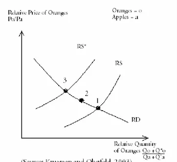
There is also David Ricardo’s Law of Comparative Advantage, which explains that a country imports the goods that are relatively more efficient to produce abroad and exports the goods that are relatively more efficient to produce domestically than abroad (Sloman, 2000). The outcome of trade and comparative advantage is plotted in Figure 2.1 below. The example considers that there are two countries home and foreign and both are able to produce apples and oranges but at different opportunity costs as can be seen by the production possibility frontier (inner line). Home is able to produce more oranges than apples using the same input of labour and foreign is able to produce more apples. Home has a comparative advantage in production of oranges and foreign has a comparative advantage in producing apples. When these two countries trade they are able to increase their consumption and are able to consume on the outer dotted line which means an outward shift in the production possibility frontier. (Krugman and Obstfeld, 2003)

The Law of Comparative Advantage is using labour as the only factor of production but labor is not the only factor that explains trade. The Heckscher-Ohlin model is instead focusing on the resource differences between countries when explaining trade, namely the relative factor abundance in different countries. What this means is that the model measures abundance in relative terms rather then in absolute terms. If country A (home) has 5 million workers and 10 million acres of land it has a one to two labour to land ratio. Comparing this number to country B (foreign) that has ten million workers and acres of land respectively (one to one ratio) we can see that country A is land abundant and country B is labour abundant. (Krugman and Obstfeld, 2003)

These numbers are not meaningful without introducing the terms labour- and land- intensive goods. A labour abundant country will produce a labour intensive good and vice versa. Looking at Figure 2.2, we can see the relative prices of oranges and apples. What trade does according to this model is that it converge relative prices. If the price of oranges increases (assume the oranges is the labour-intensive good produced by country B) the purchasing power of labour in terms of both goods will increase and in terms of land it will decrease for this country. In other words, the people in country B who receive their wages from production of oranges will gain from trade and the ones who receive their wages from apple production, which is the land intensive good will, become worse off. For country A, the opposite is true. In this country, which is, land abundant the people receiving wages from the apple sector will gain from trade and the ones receiving wages from the orange sector will loose from trade. This is the case since the relative price of oranges fall. Assuming that country A lies at point one in figure 2.2 and country B lies at point three before trade, we can see a convergence of the relative prices making prices end up in between, at point two. (Krugman and Obstfeld, 2003)

The Heckscher-Ohlin, like the Law of Comparative Advantage, says that there are gains to be made from trade and that is why countries trade with each other.

Trade theories like the Law of Comparative Advantage described above explain trade in the absence of any trade agreements such as the EU, which is important to recognize because they affect trade. The gravity model in its simplest form does the same, however it can be used to estimate the effects of trade agreements as often done by researchers in the area. A deeper explanation of the gravity model will be given in chapter 4 where we will present our modified version of the Soloaga and Winters (2000) model.

According to Krugman and Obstfeld (2006), the most important point of international trade is the mutual benefit to the countries engaging in trade goods and services. Countries have never been this closely linked as they are now in the 21st century and most of this has to do with the increasing rate of international trade and money flow. The goal of the establishment of the EU was to create a free trading market for its members, this chapter will be dedicated to investigate the terms trade diversion and trade creation and see whether Sweden has experienced it after joining the EU.

2.2 Trade Diversion and Trade Creation

The terms trade diversion and trade creation were first coined by Professor Jacob Viner in The Customs Union Issue (1950). He defined trade diversion as trade being diverted from efficient importers towards less efficient importers when a customs union is formed. Such a union is created when two or more countries partially or completely remove their tariff between themselves and apply a common tariff towards non-members. When a country applies the same tariff towards all countries it will always import from the most efficient producer and the most efficient country is the one that provides the goods at the lowest price.

Professor Viner (1950), states that when a customs union is formed the trading partners of the member countries will shift towards member states. The theoretical reasoning behind this is that if a member state in the union is a less cost efficient country then a country outside the union it may still be more profitable to import from that country than the more cost efficient one. The more cost efficient country is subjected to tariffs that will lead to higher costs.

Trade diversion is profitable for members within a union but for non-members, this phenomenon affects them negatively economically. A decrease in economic efficiency and surplus is created when countries tend to divert their trade to lower comparative advantage countries from a high comparative advantage country. (Viner, 1950)

According to Professor Viner (1950) trade creation is established when countries join a customs union and by doing so members in the customs union increase their trade with each other and trade is created.

Soloaga and Winters (2000) defines the terms slightly different as mentioned in section 1.1 which is the definition we will use for our thesis because we further on use their modified version of their regression model. They define trade diversion as an increase in

intra-block at the expense of extra-block trade and trade creation as intra-block trade increased above normal levels, the levels of trade if EU did not exist without any changes in extra-block trade.

3

Institutional and Empirical Framework

The third chapter gives the reader an insight of what expectations Sweden had on EU before becoming a member. The chapter also depicts Sweden’s overall trade pattern between 1985-2004 to be able to give a general view about trade diversion and creation.

3.1 The Four Freedoms and the Expectations on EU

The European Union rests on the pillars of the Four Freedoms, which is the very basic idea behind the existence of EU. In theory, they represent free mobility for goods, services and capital and people including labor. Through the four freedoms the EU is trying to establish a free single market consisting of its members who all, in theory at least, have the same trade policies towards a third party country which helps to protect the single market (Allgårdh and Norberg, 2004). It normally takes time to adjust to the market conditions but Sweden was able to adjust its trade policies to that of the union almost instantly. Sweden’s advantage compared to many of the other countries when they joined was the involvement in the European Economic AREA (EEA) (Allgårdh and Norberg, 2004). Full access to the single market was however not given until Sweden became a member of EU in 1995.

This thesis focuses on the freedom of free mobility for goods, which implies that export- and import tariffs and any other action that restricts trade are forbidden in the union (Allgårdh and Norberg, 2004). Sweden has been a member of the European Union for more than 10 years now and we are therefore going to analyze the effects this has had on our trade pattern with the other members of the Union (EU14). If this framework is valid i.e. if the ratification to open the doors to trade and be a part of EU, which should lead to economic growth, then our trade with the other members should have increased since we became members. Relatively we should be better off now then ten years ago.

In 1986, the president of EEC at that time Lord Cockfield gave Paolo Cecchini, an active member of the commission, the responsibility to create a report, which summarised the results of the different studies that had been a part of a project called “The Cost of Non Europe”. The Cecchini report was presented in 1988 and the result of the report showed that the single market would lead to a one-time increase of production level corresponding to 5.3 percent of GDP, which would take place when trade barriers would be removed (Cecchini, 1988). The mathematical estimations done in the report by SOU (1994:6) showed that if trade barriers were to be removed Sweden would gain SEK3.4 billion in profit and the welfare profit would be between SEK60 and 90 billion.

Further, according to the estimations in the same report it was said that if Sweden would have chosen to stay outside the EU single market, that action would have lead to negative consequences on both Sweden’s export and import sectors. However, if Sweden instead would join EU the overall trade to and from Sweden would increase in total. The Cecchini report (1988) showed that if trade barriers were removed and trade costs lowered between the member states, trade diversion would occur for member states and non-member states would face a decrease of 6-8 percent in their imports. This is interpreted as if Sweden joined the EU up to 8 percent of the country’s imports would be diverted from non-member states to member states (SOU, 1994:6). It was also estimated that if Sweden became a member of the EU a portion of the increased trade would spill over to an increased demand of imports, leading to new trade within the EU borders meaning that Sweden would then face trade creation.

3.2 Descriptive Data

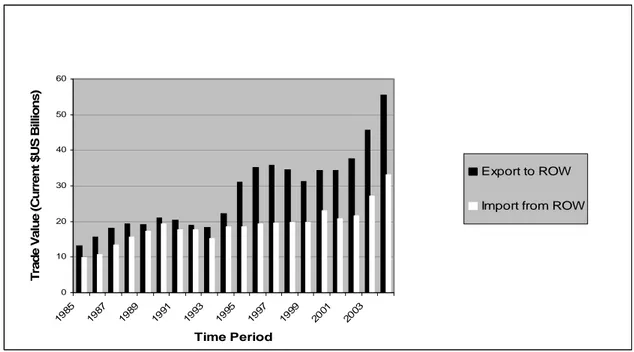
The following figures show Sweden’s trade pattern during the selected time-period 1985 – 2004. The data has been collected from the UN Comtrade database. With this data, we have created three figures. Figure 3.1 depicts Sweden’s trade pattern to the EU14 countries, Figure 3.2 depicts Sweden’s trade pattern to the Rest Of the World (ROW) excluding the EU14 countries and Figure 3.3 makes a general observation of the trade pattern to see if trade diversion has affected Sweden during the selected time period.

During this time-period (1985-2004), Sweden experienced recessions that affected the country’s trade pattern. Throughout the 1980s, the SEK was devaluated twice to improve the balance of payments and create a competitive lead for Sweden’s trade and the domestic industries. (Sveriges Riksbank, 2004)

In the beginning of the 1990s Sweden faced two large recessions which affected the trade negatively. Many Swedish companies filed for bankruptcy and this lead to cut downs in the public sector. The export at this time decreased significantly as well as the countries import. However, in 1995 Sweden’s economy was restructured which helped the country to recover from the recession. (Magnusson, 2002)

Figure 3.1 below depicts the overall trade that Sweden has had with the countries in the European Union from 1985-2004. Both the exports and imports follow a simultaneous steady upward pattern as to be expected over time. Trade value will increase over time since money is worth more today then in the future (Bade and Parkin, 2004). Two sets of anomalies can be seen in Figure 3.1 the first one is from 1991-1993 where a sharp decrease is seen, this is due to the recession that occurred at that time. The second set of anomalies can be seen from 1999-2001 but unlike the trade decrease in the beginning of the 90s there is not as clear a reason for this trade decrease. However, Sweden was still fighting the relatively high unemployment rate in the country and the IT bubble burst in 2000, which had a significant effect on the world economy. (Sveriges Riksbank, 2004)

Figure 3.1 Sweden’s Trade to EU14

0 10 20 30 40 50 60 70 80 1985 1987 1989 1991 1993 1995 1997 1999 2001 2003 Time Period Tra d e Val u e ( Curr ent$ US Bil lions ) Exports to EU14 Imports from EU14

The trade to the rest of the world in Figure 3.2 follows a different pattern compared to Figure 3.1. Our imports from ROW have not increased as much as the exports to ROW. Until the 1990s, the trade flow followed the same upward sloping pattern after which a decline can be seen until 1994. From this point in time the exports increased

significantly compared to imports. It is not until the beginning of the 21st century that the imports start to increase significantly. This is an interesting trade development because the substantial increase in exports to ROW took place right after the Swedish entrance to the EU and the trend has been increasing ever since.

Figure 3.2 Sweden's Trade to the Rest of the World

0 10 20 30 40 50 60 198 5 198 7 1989 1991 199 3 199 5 1997 199 9 2001 200 3 Time Period Tr ade V a lu e ( C ur re nt $US Bi ll io ns) Export to ROW Import from ROW

Figure 3.3 below shows the most interesting development because it lets us make a general conclusion about trade diversion and trade creation. In Figure 3.3 we can see that the share of imports from 1985 - 1990 to EU14 is slightly decreasing and is

merging with the slightly increasing share of exports to EU14, which can be an effect of the devaluations of the SEK around that time. This is consistent with economic trade theory where it is stated that if a currency becomes devaluated exports increase and imports decrease because the relative purchasing power of that country has decreased (Dornbusch, Fischer and Startz, 1997). Between 1990-1994 the share of both imports and exports remain almost the same with exports being some what lower. The

interesting part of the graph is the time-period after 1994. The share of imports to the EU14 countries has increased significantly, which implies that Sweden has diverted its imports from ROW to EU14. The share of exports has gone in the opposite direction, compare Figure 3.2 and Figure 3.3. It has decreased, implying that Sweden has diverted its exports from EU14 to ROW. Studying Figure 3.3 we conclude that Sweden has faced trade diversion and possibly some trade creation by entering the EU.

Figure 3.3 Sweden's Trade Share to EU14 (EU14/ROW)

0 0,1 0,2 0,3 0,4 0,5 0,6 0,7 0,8 1985 1987 198 9 1991 1993 1995 1997 1999 2001 2003 Time Period S h ar e: E U 14/ W o rl d EU14/World=exports EU14/world=Imports

4 Regression Model

This chapter is devoted to explain the regression model for this thesis. The model selected is the Soloaga and Winters modified version of the gravity model from 2000 which we modify to fit our purpose. The basic gravity model of trade is first explained to give the reader a clear understanding of the Soloaga and Winters model.

4.1 Gravity model of trade

The use of the gravity model of trade was first established by Jan Tinberg in 1962 (Do, 2006). The model was named after Newton’s law of gravitational attraction. The law explained that two different objects that are proportional to the product of their masses reduce with distance. When applying this model to world trade we can see that it has the same effect when including GDP and distance. The gravity model estimates the pattern of international trade and is the base point when estimating trade diversion and trade creation. (Krugman and Obsfelt, 2006)

According to Krugman and Obsfelt (2006), there is a strong empirical relationship between the size of a country’s economy and the volume of both its imports and exports. The gravity model has been used to analyse the patterns and performance of trade flow of certain time-periods. The following equation predicts the volume of trade between any two countries.

Dij Yj Yi A Tij = × ×

Where A is a constant term

Tij= trade flow, the value of trade between country i and country j Yi= is country i’s GDP

Yj= is j’s GDP

Dij= is the distance between the two countries.

The model is based on the economic size and distance of two units. To measure the economic size Gross Domestic Product (GDP) or Gross National Product (GNP) is often used. The gravity model has been used to analyse the patterns and performance of trade flow of certain time-period.

According to Do (2006), the basic model can also be converted to a linear form by using logarithms

(

)

(

)

(

)

(

)

Ln 1 2 tan

For the gravity model of trade, variables as income level, price level, language, tariffs, colonial history are often used. However, the basic gravity model is used to test more economic geography oriented issues than pure economic theories. (Do, 2006)

4.2 Model Formulation

Soloaga and Winters (2000) measure the trade effects and modifies the model from previous attempts when the gravity model has been used. Previous studies such as the one done by Frankel and Wei (1993) have used the gravity model to analyse the patters of trade flows, identifying bloc effects on both intra-bloc trade and members of the extra bloc trade. In their paper, the authors base their regression model on the gravity model but they extend it to be able to identify separate effects on the total import and export of the intra bloc. They further modify their model by testing the significance of changes in the estimated coefficients before and after formation of blocs. By using this model trade diversion, trade creation and export diversion can be estimated. However, in this paper we limit our analysis to trade diversion and creation.

Soloaga and Winters (2000) defines their model in three steps. As a first step, they define the basic gravity model shown in equation (1):

Equation (1):

[

]

Xij is the value of imports of country i from country j (i.e. exports from j to i) Ym is the Gross Domestic Product of country m

Nm is the population for country m (we exclude this variable from our regression to

decrease possible statistical errors) i

D is the average distance of country i to exporter partners, weighted by exporters’ GDP

share in world GDP, this is the “remoteness” of country i (we exclude this variable from our regression to remove statistical errors)

Dij is the distance between the economic centres of gravity (capital city’s) of the

respective countries

Ti is the land area of country m (we exclude this variable from our regression to decrease possible statistical errors)

Im is a dummy that takes value 1 when country m is an island and 0 otherwise (we

exclude this variable from our regression to decrease possible statistical errors)

Lij is a dummy for cultural affinities, this dummy shows if country iand jshare the same

language

The second step of Soloaga and Winters (2000) model is stated in equation 2 where the right hand side of equation 1 is represented by Aij which is commonly known as the anti-monde state defining trade as it would be without any PTAs. According to Bayoumi and Eichengreen 1997, Frankel (1997), and Frankel and Wei (1998) (Cited from Soloaga and Winters, 2000) the following two dummy variables P’kij and P’ki-j explain the patterns of trade diversion and trade creation.

Equation (2): j ki k kij k ij ij

A

b

P

m

P

LnX

=

+

′

′

+

′

′

Xij is the value of imports of country i from country j (i.e. exports from j to i)

Aij is the anti-monde value (the logarithm of) the trade as defined by the (log of)

equation (1) stated above.

P’kij is a dummy taking value 1 if both i and j are members of bloc k and 0 otherwise b’k is the coefficient measuring the extent to which trade is higher then expected if both i and j are member of the block (intra-bloc trade)

P’ki-j is a dummy taking value 1 if country i is a member of the bloc but j is not

m’k is the coefficient measuring the extent to which members imports from non

members are higher then expected

In the third and final step Soloaga and Winters (2000) redefines equation 2 to include export diversion i.e. when exports are diverted from ROW to other members and equation 3 states this change.

Equation (3):

+ +

= +

They further modify the variables by renaming them where

P’kij = PkiPkj P’ki-j = Pki – PkiPkj

bk = b’k - m’k

mk = m’k.

Pkm is a dummy taking value 1 if m is a member of bloc k and 0 otherwise

bk is the coefficient measuring the extent to which trade is higher then expected if both i

and j are member of the block (intra-bloc trade)

mk is a coefficient measuring the extent to which members’ imports are higher then

expected from all countries

nk is a coefficient measuring the extent to which members’ exports are higher then

expected to all countries

However, since we are only interested in trade diversion and trade creation and not export diversion we will simply use equation 2 to measure this although we do make the change in parameter P’kij and define it as PkiPkj as Soloaga and Winter (2000) does in

equation 3. The equation has been slightly modified by removing the Pki – PkiPkj dummy

variable to fit our analysis. The reason for this is that we compare two blocs, EU and ROW in our thesis compared to three blocs as Frankel and Wei (1993) and Frankel and Wei (1998) compared and nine blocs which Soloaga and Winters (2000) compared. Our model then becomes:

Equation (4): kj ki k ij ij A bP P LnX = + ij ij j i j i ij LnGDP LnGDP LnGDPC LnGDPC LnD L LnX

Where as we stated above (only modified)

PkiPkj is a dummy taking value 1 if both i and j are members of bloc k and 0 otherwise bk is the coefficient measuring the extent to which trade is higher then expected if both i

and j are members of the bloc (intra-bloc trade)

The equation below is the econometric approach we will use for our regression:

Equation (5): β ij kj ki k ij bP P B ε β α + + β +β +β +β +β + + = 1 2 3 4 5 6 7 +

Where k indicates the membership of the kth _{part of the world (In our case: EU and}

We have renamed some of the variables from Soloaga and Winters (2000) because we find them making better intuitive sense and added GDPC from Kruger (1999).

The variables we use are as follows:

i denote Sweden and j the trading partner

Xij is the value of imports of country i from country j (i.e. exports from j to i ) GDPm is the Gross Domestic Product of country m

GDPCm is the per capita gross domestic product

Dij is the distance between the economic centres of gravity of the respective countries Bij is a dummy that takes value 1 if countries i and j share a land border and 0 otherwise Lij is a dummy for cultural affinities, this dummy shows if country iand jshare the same

language

PkiPkj is a dummy taking value 1 if both i and j are members of bloc k and 0 otherwise bk is the coefficient measuring the extent to which trade is higher then expected if both i

and j are members of the bloc (intra-bloc trade)

When we analyse the regression results, if bk decreases and increases by the same amount in our two regressions pure trade diversion would take place meanwhile trade creation would be indicated by bk having a higher positive value in our 2nd regression then the decreasing bk in our 1st. However, the important measurement of trade diversion and creation is the positive and negative values of the coefficient.

It is worth mentioning that in the Soloaga and Winters (2000) model, after pooling the data, they add a real exchange rate variable since exchange rates changes over time. We have chosen to exclude this variable from our modified model due to the model

becoming more complex and the difficulties of finding the correct data. Nevertheless, we will consider this in our analysis.

4.3 Variable formulation

Dependent variable

Import, Xij, is the only dependent variable in our regression. According to Bade and

Parkin (2004) imports are goods and services bought from other countries. The import is provided for domestic consumers by foreign producers. The import variable is Sweden’s import of goods from the selected observation countries and in effect, the observation countries export to Sweden. We excluded oil products when we gathered this data from UN Comtrade due to its significant effect on trade it has for some countries such as Norway and Saudi Arabia.

The import data for Belgium and Luxembourg was reported together in the Comtrade database from 1985 – 1998. To be able to get separate data for Belgium and Luxembourg we added the import data from 1999-2004, we then calculated the percentage share of imports for the respective countries each year and then calculated the average percentage share of imports for the time-period 1999-2004. This percentage share was then used to compute the imports for Belgium and Luxembourg (1985-1998).

Independent variables

Gross domestic product, GDP (i,j), is the first independent variable in the regression.

GDP stands for the total value of all final goods and services produced in a certain country within a certain time-period. The variable is used in this model because it represents the income of a country and thereby the purchasing power. According to Nellis and Parker (2004) a country’s purchasing power shows how much trade a country have dealt with during a certain time period, hence there is a positive relationship between trade and GDP. The data for all selected years has been collected from the

United Nation Statistical database and shown in the current US dollar rate.

GDP per capita, GDPC, the second independent variable is measured by dividing the

countries GDP by its population; this gives an idea of the countries’ average wealth, which is positively correlated with trade (Bade and Parkin, 2004). The data for all selected years has been collected from the United Nation Statistical database and shown in the current US dollar rate.

Distance, D, is the third independent variable in the regression. It gives a strong

influence when determining the trade flow. Distance is connected with transportation costs and transaction costs. According to Barkman, Garretsen and Marrewijk (2001), distance and trade are negatively correlated. This means that the further the distance, the higher the cost of trade. The distance data have been collected from the Time and Date

AS webpage.

Dummy variables

Border, B, is the first dummy variable. Countries that share borders with each other

have a lower transportation cost leading to higher trade meaning a positive relation to trade (Barkman, Garretsen and Marrewijk, 2001). Sweden’s border countries are Norway and Finland. Border countries are coded as 1 and non-border countries are coded as 0.

Language, L, the second dummy variable is used to measure the common cultural

factors. Language is considered as a barrier of communication. If countries share the same language it is believed that the barriers of communication is lower and that there will be more trade, than between countries that don’t share a common language (Hacker and Johansson,2001). This means that language has a positive relation to trade.

The dummy variable is coded with either 1 or 0. 1 if countries share the same official language or 0 if Swedish is not the official language of the trade partner. In our case, we have Sweden as our point of reference and Swedish as the official language to consider. However, there is no country shearing the same official language as Sweden. We are

imposing a modified version of the language variable where we include Norway, Denmark and Finland. We include Finland since it has Swedish as an official language (CIA The world fact book, 2006).

Bloc Dummy, PkiPkj, is the third dummy variable in our regression. We have one

customs union that we will investigate which is the European Union. According to Bowen, Hollander and Viaene (1998) free trade agreements are created to increase the trade, and one of the European Unions primary goals is to eliminate any trade barriers to be able to increase wealth and economic growth of the member states (Allgårdh and Norberg, 2004). The PkiPkj dummy variable is coded as 1 and 0. 1 if both Sweden and

the trading country is a member of the bloc and 0 if not. The bloc changes over time (see Table 4.1 below). The dummy variable is expected to have a negative relation to trade during the time-period 1985-1994, and a positive relation to trade during 1995-2004.

Table 4.1 Block dummy, PkiPkj

Member status/Year 1985-1994 1995-2004

Members of ROW 1 0

5 Regression

analysis

Chapter five presents the regression analysis. Three statistical tests are done on the data and the results from the individual and joint hypothesis tests are presented.

To be able to find out if Swedish trade has face trade diversion or trade creation or both after entering the EU, several different variables are tested in our regression analysis. The most important variable for this analysis is however the bloc dummy variable

pkipkj.

The hypothesis we are testing in this thesis is:

0 .... : H 0 ... : H 8 . 2 1 1 8 2 1 0 ≠ ≠ ≠ ≠ = = = = β β β β β β

Where the null hypothesis H0 shows that there is no difference between theβ values. The alternative hypothesis H1 shows that there is a difference between theβ s. By using the modified Soloaga and Winters model (2000) two separate regressions using pooled panel data are tested to estimate the effect of the membership. Each regression is run as an OLS log linear regression testing at a 5 percent significance level and a critical t-value of 1.96. (Gujarati, 2003)

Although we know that panel data is a very complex method to estimate data and due to this the results obtained from panel data regressions can be distorted we will still use panel data. We do this because one, the Soloaga and Winters (2000) model is doing the same and their model is our point of reference and two, we estimate 45 countries over twenty years using eight different variables making it a cross-sectional, time series regression i.e. panel data. We also pool the data over time in accordance with Soloaga and Winters (2000).

5.1 Individual Hypothesis test

The first step in our regression analysis is to verify that our independent variables, when tested independently against our dependent variable are in fact correlated. Table 5.1 summarizes the relationship between the explanatory variables and the dependent variable by stating a hypothesis for each of the variables.

Table 5.1 Hypothesis for explanatory variables X1=GDPi H0:β1≤0 H1 :β1>0 X2=GDPCi H0:β2≤0 H1 :β2>0 X3=GDPj H0:β3≤0 H1 :β3>0 X4=GDPCj H0:β4≤0 H1 :β4>0 X5=Distance H0:β5≥0 H1 :β5<0 D1=Language H0:β6≤0 H1 :β6>0 D2=Border H0:β7≤0 H1 :β7>0 D3= Bloc dummy pkipkj (1985-1994) H0:β8≥0 H1 :β8<0 D3= Bloc dummy pkipkj (1995-2004) H0:β8≤0 H1 :β8>0 (Note: i = Sweden and j = trading partner)

By running an Ordinary Least Square (OLS) regression for each of the variables (8 regressions) we can present the results is table 5.2 and 5.3 respectively for our 2 time-periods.

Table 5.2 Individual Variable Testing (1985-1994)

Variable Coefficient Std. Error P-value R-squared

X1=GDPi 0.810624 0.126279 0.0000 0.011323 X2=GDPj 1.009540 0.014300 0.0000 0.580735 X3=GDPCi 0.844359 0.132222 0.0000 0.011207 X4=GDPCj 0.781240 0.019273 0.0000 0.313508 X5=Distance -1.021971 0.030548 0.0000 0.237258 D1=Language 2.762497 0.129875 0.0000 0.111699 D2=Border 2.642316 0.160873 0.0000 0.069750 D3=Bloc dummy pkipkj -2.023098 0.070030 0.0000 0.188280

All explanatory variables in table 5.2 are significant at the 5 percent significance level, as shown by the respective P-values and we do not reject any of the null hypothesis’ stated in table 5.1.

Table 5.3 Individual Variable Testing (1995-2004)

Variable Coefficient Std. Error P-value R-squared

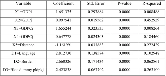
X1=GDPi 1.651375 0.297884 0.0000 0.008488 X2=GDPj 0.997541 0.019562 0.0000 0.452929 X3=GDPCi 1.655244 0.323535 0.0000 0.008264 X4=GDPCj 0.647778 0.024303 0.0000 0.184460 X5=Distance -1.161991 0.033883 0.0000 0.272429 D1=Language 2.812730 0.138574 0.0000 0.102948 D2=Border 2.660326 0.171434 0.0000 0.062861 D3=Bloc dummy pkipkj 2.423838 0.067702 0.0000 0.263100

By running the explanatory variables separately, we can confirm that each of these variables correlates correctly with the dependent variable according to the model. The independent variables, which are assumed to be positively correlated with the dependent variable, are positively correlated, and the same is true for the independent variables that are supposed to be negatively correlated with the dependent variable. Before we go on to the joint hypothesis test we will check if there is any statistical errors.

5.2 Statistical Errors

The first test that will be done to see if there are any errors in the data set is autocorrelation. Autocorrelation is defined as correlation between members of series of observations ordered in time or space (Gujarati, 2003). By looking at the Durbin-Watson statistic (d-stat) for both time periods it is concluded that there are some minor negative autocorrelation. As a rule of thumb, there is no autocorrelation when the Durbin-Watson statistic is 2, the closer the d-statistic is to 0 the more positive autocorrelation exists in the data set and the closer to 4 the more negative autocorrelation exists. The Durbin-Watson statistic in our two datasets are 2.37 and 2.43 respectively showing some negative autocorrelation indicating that the problem of autocorrelation is small.

By testing the equality of variances between series for both datasets, we conclude that there is no heteroscedasticity present in either. Since heteroscedasticity is not present, we are able to run a joint hypothesis test of our null hypothesis using OLS instead of a Generalized Least Square (GLS) analysis, which would be used if heteroscedasticity existed in the datasets (see Appendix 2 for the results of the heteroscedasticity tests). In general, signs of multicollinearity in a data set can be seen when the R-squared is high (0.8), the F-test is significant but few or none of the individual t-tests are significant (Gujarati, 2003). Running our regression we found that we had some problems with multicollinearity especially between the X1 (GDPi) and X3 (GDPCi)

variables namely X1 (GDPi) and by doing so we were able to decrease the level of

multicollinearity in the data sets. Although dropping a variable may lead to specification bias or specification errors (Gujarati, 2003) this did not affect the results notably and since we focus on trade diversion and trade creation which is estimated by D3 (Bloc dummy) which did not change at all, the regression is still reliable.

5.3 Joint Hypothesis test

A joint hypothesis test will be done to determine if the null hypothesis can be rejected and thereby verify if there is any correlation between the dependent variable and the independent variables. The joint hypothesis test will be done for both data sets and the results are presented in Table 5.4 and 5.5.

The new hypothesis after dropping variable X1(GDPi) is now:

0 .... : H 0 ... : H 8 . 3 2 1 8 3 2 0 ≠ ≠ ≠ ≠ = = = = β β β β β β

Table 5.4 Joint Hypothesis test (1985-1994)

Included observations: 450

Variable Coefficient Std. Error t-Statistic Prob.

X2=GDPj 0.895761 0.010955 81.77097 0.0000 X3=GDPCi -0.056671 0.062081 -0.912860 0.3614 X4=GDPCj 0.202044 0.013045 15.48857 0.0000 X5=Distance -0.452975 0.024090 -18.80380 0.0000 D1=Language 1.222703 0.114046 10.72113 0.0000 D2=Border 0.440941 0.139698 3.156390 0.0016 D3=Bloc dummy pkipkj -0.581225 0.048832 -11.90245 0.0000

F-value: 1989.822 R-square: 0.815943

At the 5 percent significance level the critical F-value is 2.01 (df 7, ∞) and our observed F-value is 1989.822 for table 5.4. Due to the observed F-value being higher than the critical F-value the null- hypothesis is rejected. The R-square value is 82 percent implying that the sample regression line fits the data well (Gujarati, 2003).

The critical t-value at the 5 percent significance level is 1.96 (df ∞). All the t-values in the data set are significant except X3 (GDPCi), 0.3614 > 1.96 implying that X3 and the

Table 5.5 Joint Hypothesis test (1995-2004)

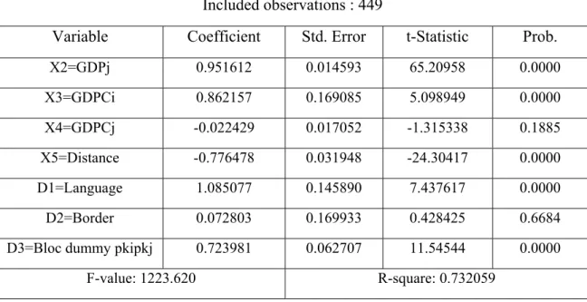
Included observations : 449

Variable Coefficient Std. Error t-Statistic Prob.

X2=GDPj 0.951612 0.014593 65.20958 0.0000 X3=GDPCi 0.862157 0.169085 5.098949 0.0000 X4=GDPCj -0.022429 0.017052 -1.315338 0.1885 X5=Distance -0.776478 0.031948 -24.30417 0.0000 D1=Language 1.085077 0.145890 7.437617 0.0000 D2=Border 0.072803 0.169933 0.428425 0.6684 D3=Bloc dummy pkipkj 0.723981 0.062707 11.54544 0.0000

F-value: 1223.620 R-square: 0.732059

The critical F-value for the second data set presented in table 5.5 is also 2.01 (df 7, ∞) at the 5 percent significance level and our observed F-value is 1223.620. The null-hypothesis is also rejected in this test. The R-square value is 73 percent implying that the sample regression line fits the data well but not as well as the R-square value for table 5.4.

The critical t-value at the 5 percent significance level is 1.96 (df ∞). All but two t-values in the data set are significant which are X4 (GDPCj) and D2 (Border), they are not

6

Analysis and Conclusion

This chapter presents the analysis and the conclusion. To be able to analyze the regression results, an equation from the Soloaga and Winters (2000) model is used to convert the statistical figures into percentage form.

There have been many debates regarding whether or not Sweden’s trade has gained or lost from the EU membership. We are now able to shed some additional light to this discussion. After joining the EU Sweden faced many changes particularly within trade, these changes have however been for the better. In the end of the 1980s when the Cecchini report was released it was concluded that creating an single market within the EEC would bring gains for member states such as increased trade, one time increase in the countries GDP and better trading relations overall and the SOU report (1994:6) stated the same thing.

When doing the descriptive analysis we found that the trade pattern had changed significantly since the entrance. The data showed that Sweden diverted their trade from non-members to member states gradually meaning that the free trade in the union had resulted in more trade with the union members. However, to determine whether this was due to better or cheaper products is difficult to establish because the tariffs on goods coming to Sweden from non-members make it very complex. Our econometric results also supported the previous studies mentioned above. Sweden gained from its membership, at least when studying trade of goods.

To be able to get any comparable results from our regression analysis we need to calculate the percentage change in trade to ROW and EU, which is done by applying the dummy variable for trade diversion and trade creation D3 in to the following equation:

[exp(dummy variable)-1]*100 (Soloaga and Winters, 2000)

This estimation showed a 44 percent decrease in imports during the time-period of 1985-1994 meaning that the overall import during these years decreased. The same dummy but for the time-period 1995-2004 shows that imports have increased by 106 percent to EU member states since 1995. This does not imply that the decrease in trade in the first period is due to the increase in trade in the second period. Observe that we are comparing two time-periods, which means that a straight comparison between the two numbers is not possible.

The decrease in the first period is not affected by the second period. We can however conclude that trade to ROW has decreased significantly in the first period and the trade to EU has increased even more in the second period showing signs of trade diversion and trade creation. The first period shows a 44 percent decrease and the second shows a 106 percent increase. If the percentage change was the same for both periods (the decrease for the first was the same as the increase in the second) it would conclude that only trade diversion has taken place. However, since the increase supersedes the decrease by 62 percent we have to conclude that Sweden has faced not only trade diversion but also trade creation after joining the EU. However, claiming that 62 percent trade creation has occurred would be incorrect because we are comparing two time-

periods as mentioned above. Here we also have to take the change in the exchange rate over time into account. Sweden’s exchange rate has changed notably during our selected time-period increasing the trade over time supporting the previous claim that as much as 62 percent trade creation has not occurred, the actual number is in fact lower. This also shows that Sweden faced trade diversion before entering into the union indicating that this can be due to Sweden having favourable trade agreements with the EU through the membership in the EEA.

When entering in to the EU a country needs to adjust its trade policies and have government finances in order among other things and the process takes a while depending on the country, implying that before applying for the membership a country needs to make adjustments. Note that countries tend to trade more with countries located close to them and with countries having a similar cultural background, (represented in our model by the dummy variables B and L). Taking into account the adjustment process mentioned above, it may explain some of the trade pattern before the membership to EU.

It would be favourable for our discussion to be able to mention an exact percentage figure regarding trade diversion and compare that to the 6-8 percent of trade diversion forecasted by the SOU report (1994:6), however it is difficult to do so. One obstacle being that if the method used to get the figures differs we are bound to get unreliable conclusions if making that comparison. Another thing worth mentioning is that we are analyzing the effect over a twenty-year period using pooled panel data, which is a complex but in our case necessary method and therefore the straight comparison is not feasible.

However, after writing this paper we are now able to conclude that Sweden has diverted its trade from non-members to member states of the EU. We can also clearly see that trade has increased to the EU countries implying trade creation and financial gains from the membership and perhaps a verification that the decision of becoming a member state of EU gave Sweden a better trading position then before.

7

Suggestions to further research

A wide range of further research possibilities in the area is presented.

The scope of further research within this subject is very wide. First, we would suggest other forms of regression analysis of the same problem for example cross sectional analysis comparing two or several smaller time-periods. Also including an exchange rate variable into the regression will give a more definite conclusion since that will consider the exchange rate.

The second suggestion is to investigate if any of the EU members who joined EMU have faced trade diversion or creation and analyze if there is any change. It might also be interesting to study if Sweden’s economy has been affected by not joining the EMU. Third, studying how much the EU can expand itself before becoming to big to function effectively. A more complex version of this study can be to research whether it is possible for EU to become a federal state and function similar to the US. Would there be any gains from such a federation? Would countries be willing to surrender their sovereignty?

Fourth, it might be interesting to research how the other “freedoms” services, capital and labour have been affected by Sweden’s membership in the EU. Such a paper might shed even more light whether the union is a success or a failure from Sweden’s point of view.

Fifth, we recommend studying not only Sweden but also how other EU countries have been affected by their respective membership. It will give a clearer picture of the effects since no country have entered the union under the same conditions. Countries differ when it comes to the economy, the political and social structure among other things. Finally, we suggest studying how the recent expansion of the EU with the ten new members has affected the EU15 members. Expanding the union with almost 70 percent must have had a significant impact on the other members.

References

Books

Allgårdh, O. and Norberg, S. (2004) EU och EG-rätten; En läro- och handbok om EU

och i EG-rätt. 4e upplagan. Stockholm: Norsteds Juridik AB

Bade, R. and Parkin, M. (2004) Foundations of Macroeconomics. 2nd ed. Boston: Pearson Addison-Wesley

Barkman, S. Garretsen, H and van Marrewijk, C. (2005) An introduction to

geographical economics, Cambridge:Cambridge University Press

Bowen, H. Hollander, A and Viaene, J. (1998) Applied international trade analysis, Basing-stoke : Macmillan

Cecchini, P. (1988) Europas Inre Marknad 1992, Stockholm: SNS Förlag

Dornbusch, R. Fischer, S. and Startz, R. (2004) Macroeconomics. 9th _{ed. Boston:} Mcgraw-Hill/Irwin

Gujarati, N.D. (2003) Basic econometrics. 4th ed. Boston: McGraw Hill

Hacker, S. and Johansson, B. (2001) Sweden and the Baltic Sea Region : transaction costs and trade intensities. In Bröcker. J and Herrman Hayo, ed. Spatial change and

interregional flows in the intergrating Europe: essays in hounoir of Karin Peschel.

Heidelberg: Physica-Verlag

Howse, R. and Trebilcook, M. (1999) The Regulation of International Trade. 2nd ed. London: Routledge

Krugman, P.R. and Obstfeld, M. (2003) International Economics Theory and Policy. 6th ed. Boston: Addison Wesley

Krugman, P.R. and Obstfeld, M. (2006) International Economics Theory and Policy. 7th ed. Boston:Addison Wesley

Magnusson, L. (2002) Sveriges ekonomiska historia, Stockholm: Rabén Prisma

Nellis, J. and Parker, D. (2004) Principles of macroeconomics. Harlow: Financial Times Prentice Hall.

Sloman, J. (2000) Economics. 4th ed. Harlow: Financial Times Prentice Hall.

Viner, J. (1950) The customs union issue, New York: Carnegie endowment for International Peace

Internet:

20061120STO00010-2006-20-11-2006/default_sv.htm Retrieved: 2006- 11-20

SCB - Statistiska Central Byrån. (Updated: 2006-06-01) Export och import av varor

fördelade på länder [online]. Available from:

http://www.europarl.europa.eu/news/public/story_page/008-11-324-11-47-901-20061120STO00010-2006-20-11-2006/default_sv.htm Retrieved: 2006- 11-20

Sveriges Riksbank. (Updated: 2004-03-11) 1900-talet [online]. Available from:

http://www.riksbank.se/templates/Page.aspx?id=9139 Retrieved : 2006- 10-18

Time and Date AS. (Updated: 2006-12 ) Calculate distance between two locations

[online]. Available from: http://www.timeanddate.com/worldclock/distance.html Retrieved : 2006- 12-16

United Nations. (Updated: 2006) UN Comtrade Database [online]. Available from: http://comtrade.un.org/db/dqQuickQuery.aspx Retrieved : 2006- 10-08

Papers

Do, T. (2006) A gravity model for trade between Vietanm and Twenty-three European

countries, D-thesis, Falun: Högskolan Dalarna

Frankel, A.J. and Wei, S.J. (1993) Trade Blocs and Currency Blocs, Working paper No. 4335, Cambridge

Frankel, J. A. and Wei, S.J. (1998) Regionalization of World Trade and Currencies:

Economics and Politics. Chicago: University of Chicago Press

Krueger, A. O. (1999) Trade Creation and Trade Diversion under NAFTA, Working Paper # 7429. Cambridge: National Bureau of Economic Research

Soloaga,I. and Winters, L.A. (2000) Regionalism in the Nineties: What Effect on Trade? Washington: World Bank

Report

Statens offentliga utredningar, (1994:6), Sverige och Europa : en samhällsekonomisk

konsekvensanalys : betänkande / av EG-konsekvensutredningen Samhällsekonomi.

Appendix 1

11 Denmark ₃₄ Republic of Korea

12 Finland ₃₅ Romania

13 France ₃₆ Saudi Arabia

14 Germany ₃₇ Singapore

15 Greece ₃₈ Spain

16 Hong Kong SAR of China ₃₉ Switzerland

17 Hungary ₄₀ Thailand

18 India ₄₁ Turkey

19 Indonesia ₄₂ United Kingdom

20 Iran (Islamic Republic of) ₄₃ United States

21 Ireland ₄₄ Venezuela

22 Israel ₄₅ Vietnam

Appendix 2

Heteroscedasticity test1985-2004

Method df Value Probability Bartlett 6 4.54E-13 1.0000 Levene (6, 3143) 2.62E-29 1.0000 Brown-Forsythe (6, 3143) 2.52E-29 1.0000

Heteroscedasticity test 1995-2004

Method df Value Probability Bartlett 6 0.000000 1.0000 Levene (6, 3136) 0.000000 1.0000 Brown-Forsythe (6, 3136) 8.99E-30 1.0000