THESIS
ANALYZING THE DETECTION EFFICIENCY OF THE GEOSTATIONARY LIGHTNING MAPPER IN ISOLATED CONVECTION
Submitted by Adam Wayne Clayton
Department of Atmospheric Science
In partial fulfillment of the requirements For the Degree of Master of Science
Colorado State University Fort Collins, Colorado
Spring 2021
Master’s Committee:
Advisor: Steven Rutledge Co-Advisor: Steven Miller Christine Chiu
2
Copyright by Adam Wayne Clayton 2021 All Rights Reserved
ii ABSTRACT
ANALYZING THE DETECTION EFFICIENCY OF THE GEOSTATIONARY LIGHTNING MAPPER IN ISOLATED CONVECTION
The Geostationary Lightning Mapper (GLM) flying on GOES-16 and GOES-17 has provided near-hemispheric lightning detection for nearly two years. Since operation began, several attempts have been made to compare flash rate observations from GLM against ground-based lightning detection systems. While GLM captures a high percentage of flashes in the field-of-view of GOES-16 and GOES-17, some studies have shown reduced detection efficiency at storm-scale. The problem of analyzing lightning from space is a complex one. Several factors such as: flash area, flash length, cloud water and ice contents, flash height, flash brightness and position relative to satellite nadir affect the detection efficiency of GLM. This study analyzes numerous convective cells in the Alabama, Colorado, and W. Texas regions to further analyze the detection efficiency of GLM. Lightning data from VHF-based lightning mapping arrays (LMAs) in each region were compared directly to measurements from GLM. The GLM/LMA ratio for each cell was computed during the lifetime of the thunderstorm. Additionally, graupel echo volumes, precipitation ice water paths, and cloud ice and cloud water paths were calculated to access the microphysics of each cell. This study features an in-depth analysis of thunderstorms that vary in size and severity from each region. Further, a statistical analysis of all of the
iii
This study found that flash rate, flash brightness and near cloud-top water and ice water paths significantly affect GLM detection efficiency. Specifically, thunderstorms with increased flash rates, cloud-top water paths, and decreased flash size/brightness are often characterized by low (< 20%) GLM detection efficiencies. These characteristics are common in so-called
“anomalous” charge structure thunderstorms that frequent the northern Colorado region.
Additionally, this study confirmed results from previous studies which found that the GLM DE decreases as the distance from nadir increases. These results will be helpful for meteorologists utilizing GLM observations to assist with decisions regarding severe weather.
iv
ACKNOWLEDGEMENTS
First, I would like to thank my advisor Dr. Steven Rutledge who gave me the opportunity
to come and study atmospheric science at Colorado State University. Steve has taught me how to be a scientist and his kind words have motivated me to push through challenges in my research. I have no doubt that Steve’s guidance has made me a better scientist and I am excited to see what I can accomplish from my experiences here. Next, I would like to thank Kyle Hilburn, Dr. Brenda Dolan, and Dr. Brody Fuchs. Kyle Hilburn was instrumental in helping me complete this
master’s thesis. Kyle helped me with many questions about coding and would always go the extra mile to help me. Kyle served as an unofficial research mentor for me and I am forever grateful for the assistance he gave me. Dr. Brenda Dolan was vital in helping me learn various radar processing techniques. Without her assistance, I would not have been able to work through all of the radar data that is presented in this thesis. I know that I will continue to rely on Dr. Dolan’s radar knowledge throughout my career. Dr. Brody Fuchs and Karly Reimel were instrumental in helping me learn the CLEAR cell tracking code. I am excited to be able to pass down their knowledge to other scientists who are interested in the code. I would also like to thank Paul Hein who was always able to help with any IT problems that I encountered. Next, I would like to thank the other students who were in the Rutledge Group while I was there: Kyle Chudler, Marqi Roque, and Joe Messina. Thank you for being kind and welcoming me to the group. I would also like to acknowledge the rest of my committee members: Dr. Steven Miller, Dr. Christine Chiu, and Dr. Richard Eykholt. Finally, I would like to thank the friends I made along the way at Colorado State. This is a special place full of special people and I am happy to say that I made memories that I will never forget.
v
TABLE OF CONTENTS
ABSTRACT...ii
ACKNOWLEDGEMENTS...iv
Chapter 1. Introduction...1
1.1 Geostationary Lightning Mapper………...1
1.2 Lightning Charge Separation……….2
1.3 Anomalous Charge Structure Thunderstorms...6
1.4 Goals of This Study...8
Chapter 2. Data and Methodology...10
2.1 Radar Data...10
2.2 Hydrometeor Identification...11
2.3 Ice Water Path...11
2.4 Cloud Top Water Path...12
2.5 Lightning Data...13
2.5.1 Geostationary Lightning Mapper...13
2.5.2 Lightning Mapping Array...14
vi
2.6 CLEAR...16
Chapter 3. Case Studies...20
3.1 Case Selection...20
3.2 Colorado Cases...20
3.2.1 July 1st, 2019 Normal Thunderstorm...20
3.2.2 May 26th, 2019 Normal Thunderstorm...24
3.3.3 May 26th, 2019 Anomalous Thunderstorm...27
3.3 West Texas Cases...30
3.3.1 April 23rd, 2019 West Texas Case...30
3.3.2 May 5th, 2019 West Texas Case...32
3.3.3 June 24th, 2019 West Texas Case...35
3.4 Alabama Cases...38
3.4.1 May 17th, 2020 Alabama Case...38
3.4.2 July 4th, 2020 Alabama Case...40
3.4.3 April 8th, 2020 Alabama Case...43
3.5 Summary of Cases...46
Chapter 4. Statistical Results...47
vii
1
CHAPTER 1: INTRODUCTION
The Geostationary Lightning Mapper (GLM) aboard GOES-16 and GOES-17 has been providing real-time near-hemispheric lightning detection for nearly four years. The GLM observations have provided insight into the lightning observations of many atmospheric processes ranging from hurricanes to volcanic eruptions. The lightning data has also assisted meteorologists in forecasting severe weather and the impacts of thunderstorms on life and property. Now that a large sample size of thunderstorms has been observed by the two GLM platforms, it is important to access the performance of GLM, in particular, flash rate. The key measurement here is the detection efficiency of GLM, formed by taking the ratio of the GLM flash rate to the flash rate from other lightning locating systems (LLS) over the same storm area. This thesis focuses on assessing the detection efficiency of the GOES-16/17 GLM within
isolated convection. Detection efficiency is obtained from VHF based Lightning Mapping Array data. Numerous case studies of thunderstorms in different regions are analyzed in this study to identify factors that affect GLM’s ability to detect flashes. Additionally, a statistical investigation is performed to draw more generalized conclusions from the thunderstorms that were observed. 1.1 GEOSTATIONARY LIGHTNING MAPPER
The GOES-16 satellite was launched on 19 November 2016 and moved into its
operational position of 75.2 W on 18 December 2017. GOES-17 followed on 1 March 2018 and reached its operational position of 137.2 W on 12 February 2019. Together, they have provided real-time near-hemispheric lightning observations for nearly two years via the Geostationary Lightning Mapper (GLM). GLM is a near-infrared optical transient detector that detects optical emissions produced by electrical breakdown processes at a wavelength of 777.4 nm. The GLM sensor employs a charge coupled device (CCD) that stares constantly at the surface of the Earth.
2
The CCD has a wide field-of-view (FOV) with a size of 1372x1300 pixels (Goodman et al. 2013). GLM provides lighting coverage up to 52 N/S latitude with a frame rate of 2 milliseconds. The pixel size of GLM varies from ~8 km at nadir to ~14 km at the edges of the FOV. The design specifications of GLM were for 70% detection efficiency over the FOV.
Since the data have become operational, several attempts to study the performance of GLM have been made. Early returns of GLM suggest that the performance of GLM met or exceeded design specifications on a hemispheric scale (Koshak et al., 2018). Another study found that measurements of GOES-16 GLM meet design specifications in most locations except for the western Great Plains region (Marchand et al. 2019). Further work found that GLM has a higher detection efficiency during nighttime hours when compared to the daytime (Cummins 2020). The GLM detection efficiency also decreases with increasing distance from nadir
(Cummins 2020). Further research has found that GLM has a high detection efficiency for large flashes with long durations but reduced DEs for short duration flashes with small areas (Zhang and Cummins 2020). Additionally, other studies have shown that there is reduced detection efficiency for the so-called anomalous charge structure thunderstorms that have small flashes, low flash heights, and increased cloud water paths (Thomas et al., 2019, Rutledge et al., 2020). These thunderstorms are characterized by extremely high lightning flash rates. These storms are often associated with sever weather, hail, strong winds or tornadoes. Since these thunderstorms commonly produce severe weather, it is important to determine what it is about them that causes low GLM DE.
3 1.2 LIGHTNING CHARGE SEPERATION
Electrical breakdown leading to lightning in thunderstorms is the result of particle collisions in the mixed phase region of a convective cloud which creates a separation of charge. This charge separation usually manifests itself in the form of a tripole charge structure with a negative mid-level charge layer situated between an upper and lower-level positive charge layer (Williams 1985). The charge separation occurs when small ice crystals and larger graupel particles collide and separate in the presence of supercooled cloud liquid water. The small ice crystals (normally positively charged) are lofted to the upper parts of a thunderstorm cloud while the heavier graupel particles (normally negatively charged) settle to the mid-levels (Williams et
4
al., 1989), leading to positive over negative charge in the upper half of the tripole.
Figure 1.1: Figure 8 from Takahashi et al. 1978.
The lower positive region of normal polarity thunderstorms results from hydrometeors that fall from the mid-levels of the thunderstorm and acquire positive charge. Graupel particles acquire positive charge in the lower level of the mixed phased region because graupel charges positively at higher temperatures and lower cloud water contents (Takahashi 1978, Saunders and Peck 1998, Saunders et al. 2006). The physics of charge separation have been the focal point of many laboratory studies (Reynolds et al. 1957; Takahashi,1978; Jayaratne et al. 1983; Baker et al. 1987; Saunders et al. 1991; Saunders and Brooks 1992; Saunders and Peck 1998; Mason and Dash 1999, 2000; among others). The earliest of these laboratory studies found that a graupel
5
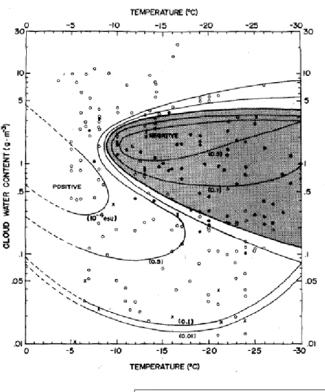
particle undergoing riming acquires a significant amount of charge when it collides with an ice crystal in the presence of supercooled liquid water (Reynolds et al. 1957). Further results established that the polarity of the charge on the riming particle varies with temperature and supercooled liquid water content (Takahashi 1978). This study showed that there was a charge reversal line related to temperature and that graupel charged positively at temperatures warmer than -10 C and negatively at colder temperatures. Also, at high liquid water content, the rimer was found to charge positively regardless of temperature. Additionally, this study found that varying amounts of cloud water content can affect the polarity of charge on the graupel particle (Figure 1.1). While most studies show that the charge reversal line exists, many disagree on what the actual temperature is. Figure 1.2 shows the different results for the charge reversal line from Takahashi (1978), Saunders and Peck (1998), Pereyra, Avila, Castellano and Saunders (2000), and
6 Saunders et al. (2006).
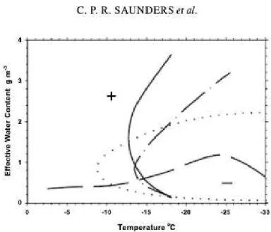
Figure 1.2: Figure 13 from Saunders et al. 2006. The original caption is included in the above figure.
Each study shown in Figure 1.2 shows that the charge reversal line varies based on the effective cloud water content. All studies show that graupel can charge positively at warmer temperatures so long as the cloud water content is increased. However, all of these studies disagree on the relative location of the charge reversal line. Still, another study found that the charge reversal line is -20 C (Jayaratne et al. 1983). The charging on a graupel particle is still very much an ongoing research question.
The non-inductive charging theory is the most accepted idea for lightning in thunderstorms. Baker and Dash 1994 theorize that a quasi-liquid layer (QLL) surrounding the ice particle is responsible for the charge transfer. The QLL is comprised of an outward negative charge (OH-)
and an inward positive charge (H+) ions. When two ice particles with different QLLs interact
7
chemical equilibrium is established between both QLLs (Dash et al., 2001). The negative charge moves in the direction of this mass transfer, therefore the particle with thinner QLL will acquire net negative charge and the particle with the thicker QLL acquires net positive charge (Dash et al., 2001). The study states that negative charge moves from higher temperature to lower temperature, high surface curvature to low surface curvature, and high vapor growth rate to lower vapor growth rate. In the mid-layer of a thunderstorm, graupel is typically growing by riming while ice crystals are growing due to vapor deposition. Therefore, the graupel particle acquires net negative charge according to Baker and Dash (1994) and Dash et al. (2001).
1.3 ANOMALOUS CHARGE STRUCTURE THUNDERSTORMS
The typical thunderstorm archetype explained in Williams et al., (1989) describes a thunderstorm with a mid-layer negative charge region sandwiched between a lower-level and upper-level positive charge region. This charge structure promotes intra-cloud (IC) flashes between the mid-level negative region and the upper-level positive region. This charge structure also promotes negative polarity cloud-to-ground lightning strikes (-CG). While -CG strikes make up the majority of CG strikes in the United States (Orville 1994, Zajac and Rutledge 2001), there are a subset of thunderstorms in the U.S. that produce predominately +CG strikes (Boccippio et al. 2001; Carey et al. 2003; Williams et al. 2005; Fuchs et al. 2015). Zajac and Rutledge (2001) and Boccippio et al. (2001) found that the largest percentage of +CG strikes occur in the high plains region from Colorado to North Dakota and Minnesota. These studies also found that the majority of high +CG flash rate thunderstorms occur in the same region. Numerous studies have also shown that positive polarity CG’s are more likely to occur in thunderstorms that produce severe weather (e.g. Branick and Doswell 1992; Carey and Rutledge 1998; Lang et al. 2002, 2004; Carey et al. 2003; Wiens et al. 2005; Tessendorf et al. 2007).
8
The presence of +CG lightning strikes has been linked to the so-called “anomalous” charge structure in thunderstorms marked by the presence of a positive mid-layer charge rather than a negative charge (Carey and Rutledge 1998; Weins et al. 2005; Tessendorf et al. 2007; Fuchs et al. 2015). The reason for this difference in charge structure is not totally understood, but there have been many studies to address the physics of anomalous (or inverted) storms. Williams et al. (2005) suggest that high cloud base heights (CBHs) accompanied by small warm cloud depths (WCDs) might be the reason for anomalous charge structure thunderstorms. The idea is that shorter WCDs promote a higher supercooled liquid water content in the mixed-phase region of a thunderstorm. Thunderstorms with small WCDs are not efficient in the warm rain processes of collision and coalescence which allows for higher supercooled liquid water contents in the mixed-phase region. The elevated cloud base heights over the High Plains region also promotes wider updrafts compared to thunderstorms with low CBHs (McCarthy 1974). The combination of wide updrafts and shallow WCDs produce increased supercooled liquid water contents in the mixed phase region which are known to cause net positive charge on graupel particles (Saunders et al. 1991; Saunders and Peck 1998). When enhanced cloud water content values exist in the mixed-phase region, the graupel particle acquires the thicker QLL compared to the normal situation where the ice crystal has the thicker QLL. In this situation, negative charge flows from the graupel particle to the ice crystal and the graupel particle acquires positive charge Dash et al., (2001).
Fuchs et al. (2015) found that most thunderstorms in the Colorado region are of anomalous polarity with a mid-level positive charge region while thunderstorms in Alabama are typically of normal polarity. Another factor in the formation of anomalous charge structure thunderstorms is the warm cloud residence time, or the time an air parcel takes to move upward through the warm
9
cloud depth. Here the warm cloud depth is the vertical distance between cloud base and the freezing level. Fuchs et al. (2018) found that anomalous thunderstorms have much smaller warm cloud residence times compared to normal thunderstorms, due to the geometrically thinner WCD. It is thought that large warm cloud residence times allow coalescence to develop which works to reduce the cloud water content in the mixed phase region, resulting in negative charging of graupel (Williams et al. 2005). Shorter WCDs and stronger updrafts result in shorter warmer cloud residence times and enhanced supercooled liquid water contents in the mixed phase region which results in positive charge on the graupel particle (Takahashi 1978, Saunders and Peck 1998, Pereyra, Avila, Castellano and Saunders 2000, and Saunders et al. 2006).
Thunderstorms do not have to begin as anomalous polarity to eventually produce +CG strikes. A period called an “end-of-storm-oscillation” (EOSO) sometimes occurs during the decaying stages of a thunderstorm storm (Marshall and Lin 1992; Williams et al. 1994; Pawar and Kamra 2007; Marshall et al. 2009). The EOSO is characterized as a change of charge structure during the latter stages of a thunderstorm. Typical normal charge structure
thunderstorms are characterized by a mid-level negative charge typically situated between -15 and -20 C along with a low-level and upper-level positive charge region. When a thunderstorm begins to decay, the mid-level negative charge region becomes less prevalent and the storm is dominated by positive charge region for a time. It is during this time period that the thunderstorm cloud becomes conducive for the development of +CG strikes.
1.4 GOALS OF THIS STUDY
The overall goal of this study is to investigate GLM detection efficiency, especially focusing on what mechanisms lead to particularly low DE (< 20%) for storms occurring in certain areas. Several thunderstorms from the Alabama, Colorado, and west Texas region are
10
analyzed to study the performance of GLM. The lightning flash rates from ground-based lightning locating systems are compared to that of GLM. Additionally, several microphysical variables such as ice water path, cloud water/ice path, hail, and graupel volumes are analyzed to identify trends between thunderstorms with high GLM DEs versus those that have low GLM DEs. Questions that will be answered in this study include:
1) What factors affect the GLM DE?
2) Are low GLM DE’s limited to storms with anomalous charge structures?
3) Can GLM detect dynamical changes in lightning flash rate of severe thunderstorms? All of these questions are important for meteorologists who use GLM to forecast severe weather.
11
CHAPTER 2: DATA AND METHODOLOGY
This section will provide an overview of the data and methodologies that were used in this study. The radar dataset from NEXRAD will be described and which radars were used will be described in section 2.1. Additionally, the radar variables used in this study will be described in this section. The list of programs used to derive the hydrometeor identification will be
described in section 2.2. While the methods used to derive ice water path and cloud top water path will be discussed in sections 2.3 and 2.4 respectively. Lightning data from the Geostationary Lightning Mapper, various lightning mapping arrays, and the National Lightning Detection Network will be discussed in section 2.5. Finally, the CLEAR tracking algorithm will be discussed in section 2.6.
2.1 RADAR DATA
The Next Generation Weather Radar Program (NEXRAD) is a combined effort of the U.S. Departments of Commerce, Defense, and Transportation (Crum and Alberty 1993). The network currently consists of 160 WSR-88Ds (Weather Surveillance Radar – 1988 Doppler; or WSR-88D) throughout the United States and certain overseas locations (National Centers for Environmental Information). The main function of NEXRAD is to provide warning and
nowcasting capabilities for the National Weather Service (NWS). The WSR-88D radars operate at an S-band wavelength and simultaneously transmit and receive both horizontally and
vertically polarized electromagnetic radiation (Doviak et al. 2000). The radars scan 360 degrees azimuthally and employ multiple elevation scans. The data from any radar in the network are free to download at https://www.ncdc.noaa.gov/nexradinv/.
12
This study utilizes radar data from the KCYS site in Cheyenne, WY, the KFTG site in Denver, CO, the KHTX site in Huntsville, AL and the KLBB site in Lubbock, TX. The variables utilized in this study include reflectivity (Z), differential reflectivity (ZDR), specific differential
phase (KDP), and correlation coefficient (𝜌ℎ𝑣). Quality control is performed on the reflectivity to
remove unwanted returns such as clutter, insects, and other non-meteorological echoes using methods in CSU-Radartools ( https://github.com/CSU-Radarmet/CSU_RadarTools). Biases in ZDR as well as KDP calculation are completed using the functions in the CSU-Radartools
package. The radar data were gridded to a cartesian grid using bilinear interpolation in Radx2Grid. The resulting grid-spacing is 1x1x1 km.
2.2 HYDROMETEOR IDENTIFICATION
Hydrometeor identification (HID) is performed using the CSU-Radartools fuzzy logic HID program (https://github.com/CSU-Radarmet/CSU_RadarTools). This array of functions takes in gridded radar data and uses Z, ZDR, KDP, and 𝜌ℎ𝑣 to determine the dominant
hydrometeor type at each grid point. The freezing levels were determined by interpolating soundings from the University of Wyoming sounding archive
(http://weather.uwyo.edu/upperair/sounding.html) to the radar grid. Only data above the freezing level were considered for HID. The existence of graupel and ice crystals in the mixed phased region of a thunderstorm are integral to the production of lightning. Therefore, the hail and graupel volumes for each radar volume is calculated for the case studies in this thesis. Since the radar data is gridded on a 1x1x1 km grid, the grid points with hail and graupel are simply summed to calculate the echo volumes.
13 2.3 ICE WATER PATH
The ice water content (IWC) for each radar volume is calculated using the liquid ice mass function in the CSU-Radartools program
(https://github.com/CSU-Radarmet/CSU_RadarTools/blob/master/csu_radartools/csu_liquid_ice_mass.py). The ice mass function uses Z, ZDR, grid heights, temperature, and freezing height to calculate the ice water
content at each height for each radar volume. These variables are then used in the ice mass calculation from (Carey and Rutledge 2000):
𝐼𝑊𝐶 = 1000 𝜋 (𝜌𝜌𝑖𝑐𝑒
𝑎𝑖𝑟) 𝑁0
3 7⁄ (5.28 × 10⁻¹⁸𝑍
720 )
4 7⁄
Where IWC has units of kg m-3, 𝜌
𝑖𝑐𝑒is the density of ice (917 kg m-3), 𝜌𝑎𝑖𝑟 is the density of air in
units of kg m-3 which was calculated from sounding data, N
0 is the intercept parameter of an
assumed inverse exponential distribution for ice ( 4 × 10⁶
m
−4 is the fixed value), and Z is the linear radar reflectivity factor (mm6 m-3). The IWC is integrated vertically throughout the radar echo column to convert to ice water path (kg m-2). There are two values of IWP used in this study. The first value of IWP is IWC values that are vertically integrated from the freezing level to the 0 dBZ echo height. The second value of IWP are IWC values that are vertically integrated from the median LMA flash height for a given radar scan to the 0 dBZ echo height. This value will hereafter be referred to as AF (above-flash)- IWP. The IWP calculations discussed here pertain only to precipitation-sized ice particles, detectable by weather radar.2.4 CLOUD WATER PATH
Cloud products from the Clouds from AVHRR Extended (CLAVR-x) package are used in this study, specifically to relate cloud water path to GLM detection efficiency. Retrievals of
14
cloud optical depth (COD), cloud-top effective particle size (CPS), and cloud water path (CWP; derived from COD and CPS) are used to analyze the optical extinction of lightning flashes in the thunderstorm cases analyzed in this thesis. These products are derived from the Clouds from AVHRR Extended (CLAVR-x) retrieval saturates at a value of 1.2 kg m-2. CWP derived from COD and CPS using the following equation: CWP = (5/9)*COD*CPS. Values of CWP can be calculated as long as the optical depth is less than ~160. At larger optical depths, the CWP estimates saturate yielding no additional information between CWP| and detection efficiency.
Thunderstorms of course have large optical depths, so the true cloud water path between the location of a lightning strike and cloud-top can never be achieved using this methodology. However, since CWP is directly related to the cloud optical depth and the cloud particle size, this calculation does provide some value in determining the scattering properties of a given
thunderstorm.
Since the CWP variable characterized in this study does not always reach to the LMA flash height due to saturation, the term cloud top water path (CTWP) is settled upon to clarify. Therefore, the terminology of cloud top water path (CTWP) is adopted for this reason. The CLAVR-x files can be downloaded for free from the NOAA CLASS archive
(https://www.bou.class.noaa.gov/saa/products/welcome;jsessionid=11A58BEABA2515A6371D 86C9DD1EFE14).
2.5 LIGHTNING DATA
2.5.1 GEOSTATIONARY LIGHTNING MAPPER
The GOES-R series Geostationary Lightning Mapper (GLM) is currently operational onboard GOES-16 (East) and GOES-17 (West). GOES-16 reached its operational location of
15
75.2 W on 18 December 2017 while GOES-17 reached its location of 137.2 W on 12 February 2019. GLM is comprised of a wide field of view (FOV) lens with a 1372x1300 pixel charge coupled device (CCD) imager and detects optical emissions from lightning breakdown processes at a wavelength of 777.4 nm (Goodman et al. 2013). The size of a GLM pixel varies from 8 km at nadir to approximately 14 km at the edge of the FOV (Goodman et al. 2013). The flash detection efficiency requirement for GLM is 70% with a 5% false alarm rate (FAR). The basic unit of GLM is termed an “event,” which is the combination of all lightning pulses within an 8x8 km pixel within 2 ms. The Lightning Cluster and Filter Algorithm (LCFA) combines adjacent events into “groups” if they occur simultaneously. Then, the algorithm combines groups into flashes if the groups occur within 330 ms and 16.5 km. GOES-16 data from 17 May 2018 through 30 June 2020 were used in this study for Alabama, Colorado, and West Texas
thunderstorms. GOES-17 data were not used in the Alabama region due to the distance from the satellite’s nadir point, placing the region on the extreme periphery of its GLM FOV.
2.5.2 LIGHTNING MAPPING ARRAY
Surface-based Lightning Mapping Arrays (LMA) detect VHF radiation due to electrical breakdown processes in thunderstorms. These networks detect several VHF “sources” within each lightning flash and are thus able to adequately map the characteristics of a flash. LMAs utilize time-of-arrival (TOA) techniques to calculate the geospatial location and time of a flash. If a radiation source is received by four or more LMA sensors, then the x,y,z locations as well as time can be solved for (Thomas et al., 2004). Three LMA networks are used in this study, the North Alabama LMA (NALMA) the Colorado LMA (COLMA), and the West Texas LMA (WTLMA). Figures 1.1, 1.2, and 1.3 show the locations of the stations that are located in NALMA (Koshak et al., 2004, Goodman et al., 2004), COLMA (Rison et al., 2012), and
16
WTLMA (Bruning 2011). Figures 1.1-1.3 also show a 100 km radius from the LMA center which is the cutoff for LMA data in this study. The detection efficiency of LMAs decreases substantially beyond 125 km from the LMA center (Rison et al., 1999; Thomas et al., 2004; Fuchs et al., 2016; Chmielewski and Bruning 2016).
While LMAs provide a wealth of information regarding VHF source location, clustering of the sources is needed to obtain flash characteristics. This study takes advantage of a density- based flash-clustering algorithm (Bruning and MacGorman, 2013; Fuchs et al., 2015, 2016) to group the VHF sources into flashes. A maximum distance threshold of 3 km and a temporal threshold of 150 ms were used to cluster radiation sources in all of the networks (Fuchs et al., 2015, Eric Bruning personal communication, Timothy Lang personal communication). Flashes identified by the clustering algorithm were required to contain at least 10 VHF sources before considered a flash in the COLMA and WTLMA networks. NALMA was recently reconstructed after some of its sensors participated in the RELAMPAGO field campaign. More sensors have been added to the network since the Fuchs et al., 2015 study, so a minimum source threshold of 5 VHF sources was employed for the NALMA.
Once the flash clustering algorithm is employed on the LMA data, numerous flash statistics can be calculated. The variables used in this study include VHF source density, LMA flash rate, and LMA flash size. Additionally, this allows for LMA detected flashes to be
compared to GLM and NLDN detected flashes. Flash information from LMAs is considered to be near 100% inside the prescribed boundary of an LMA network (Fuchs et al., 2016).
17
The National Lightning Detection Network (NLDN) has provided continental lighting observations since 1989. Electrical breakdown processes produce radiation across a broad spectrum, but NLDN measures radiation in the VLF range (3-30 kHz)/LF (30-300 kHz) with a detection efficiency > 90% (Cummins et al. 1998, Cummins and Murphy 2009). While NLDN is able to detect flashes over long distances, it is not able to resolve smaller IC flashes compared to LMAs. Additionally, NLDN can sometimes misidentify IC flashes as CG flashes. Therefore, if the NLDN databases included a CG flash with a peak current less than 15 kA then it was registered as an IC flash. Additionally, if an IC flash had a peak current greater than 25 kA then it was recorded as a CG flash (Dr. Timothy Lang: personal communication).
2.5.4 Comparison Between GLM and LMA Flash Rates
The Geostationary Lightning Mapper and VHF lightning mapping arrays detect lightning in distinctly different ways. GLM measures pixel-scale optical emissions in the near IR region of the EM spectrum resulting from while LMAs measure electromagnetic “burst” radiation
produced by lightning in the VHF portion of the EM spectrum. GLM and LMA algorithms then group the native resolution data into lightning flashes. So these stark differences in detecting lightning should be kept in mind. The comparison between to two instruments was experimented some within this study. First, comparison between GLM flashes and LMA flashes with a source minimum of 10 sources was employed. This strategy includes many LMA flashes that are often too small for GLM to visualize. Thus, the minimum VHF source threshold was increased to 75 sources. Obviously, this improved the GLM detection efficiency by reducing the LMA flash rate. However, this strategy was abandoned because it was determined that small, physically realistic lightning flashes were being eliminated from the analysis. The minimum of 10 VHF sources was also used in previous studies describing LMA flash rates.
18 2.6 CLEAR
The Colorado State University (CSU) Lightning, Environment, Aerosols, and Radar framework developed in (Lang and Rutledge 2011) is used to analyze thunderstorms in this study. CLEAR consists of a series of functions that work together to track convective cells from initiation to cessation. The variables used to track convective cells are tunable. This study required a 35 dBZ reflectivity contour of at least 20 km2 and a 45 dBZ contour of 10 km2 for the
algorithm to track the thunderstorms of interest. CLEAR ingests gridded 3-dimensional radar data and writes new radar NETCDF files with the track information included. When the tracking process is completed, additional information can be attributed to the tracked cells. LMA and NLDN flash information as well as GLM flash, group, and event data are attributed to each cell in this study. These data are used to make the timeseries plots and statistical plots in the results section.
19
Figure 2.1: Plot showing the North Alabama Lightning Mapping Array (NALMA). Red boxes denote the locations of the various LMA stations while green triangles show city and radar locations.
20
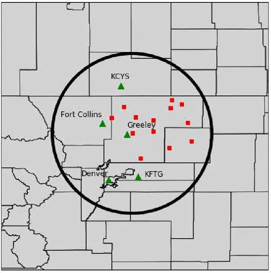
Figure 2.2: Plot showing the Colorado Lightning Mapping Array (COLMA). Red boxes denote the locations of the various LMA stations while green triangles show city and radar locations.
21
Figure 2.3: Plot showing the West Texas Lightning Mapping Array (WTLMA). Red boxes denote the locations of the various LMA stations while green triangles show city and radar locations.
22
CHAPTER 3: CASE STUDIES 3.1 CASE SELECTION
One main objective of the GOES-R series of GLM was to increase lightning detection in severe thunderstorms and increase NWS warning lead times for high impact storms. Therefore, it is important to document the performance of GLM relative to other lightning detection systems. This study focuses on isolated convection in Alabama, Colorado, and West Texas. Large
convective systems are comprised of many thunderstorm updrafts and the updraft producing the lightning can be ambiguous. Therefore, focusing on one thunderstorm cell per case study allows for a relatively simple comparison of ground lightning location systems (LMA and NLDN) to performance by GOES-16/17 GLM. Thunderstorms of different intensities are documented in each region ranging from intense, severe thunderstorms to storms with weak updrafts and modest flash rates. Additionally, since the detection efficiency of GLM varies from day to night,
thunderstorms at different times of the day were analyzed. 3.2 COLORADO CASE STUDIES
3.2.1 JULY 1, 2019
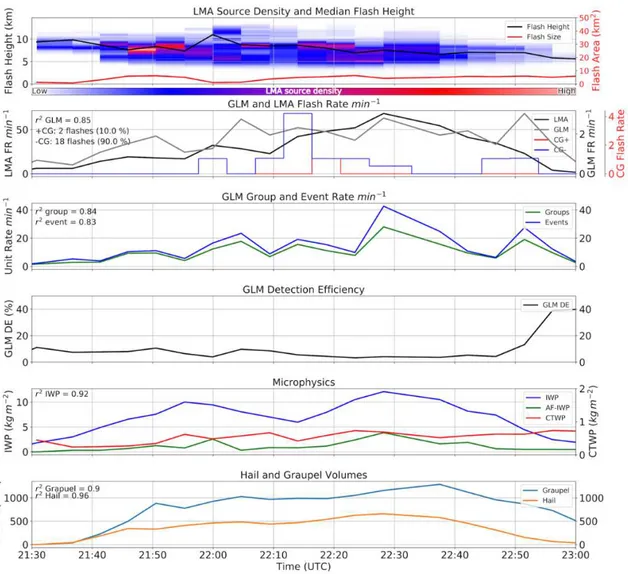
The first Colorado case presented in this study occurred on the night of 1 July 2019. The timeseries of this thunderstorm is shown in Figure 3.1 The thunderstorm initiated at 01 UTC on 2 July 2019. The top panel of Figure 3.1 shows the location of VHF radiation sources which is a proxy for the location of positive charge in a thunderstorm. Notice that the location of positive charge is located around 10 km for the entirety of the event. Since the main location of positive charge is located near 10 km and the majority of CG flashes are of negative polarity this thunderstorm likely possesses a normal polarity charge structure (Fuchs et al. 2015, Fuchs et al.
23
2016, Fuchs and Rutledge 2018). Normal polarity charge structure thunderstorms are characterized by and upper-level and lower-level positive region with a negative charge layer in the middle (Williams et al. 1989, Fuchs et al. 2015). Additionally, the flash areas are relatively large during this thunderstorm with values > 20 km2 (Bruning et al. 2013).
Panel 2 shows the LMA, GLM, and NLDN flash rates in flashes min-1, flashes min-1, and
flashes per 5 min-1 respectively. Note that these flash rates are all on different axes. The GLM flash
rate is mainly larger than the LMA flash rate until about 0125 UTC. This thunderstorm reaches a maximum COLMA flash rate of around 8 flashes per minute near 0130 UTC. This is one of the few Colorado cases in this study where the GLM flash rate has a similar magnitude than that of the COLMA flash rate. This thunderstorm was of normal polarity with 97.5% of the CG flashes being negative. The GLM group and event rates also have a high correlation to the LMA flash rate. There is an interesting increase in the GLM flash, group, and event rate at approximately 0200 UTC which correlates to an increase in LMA flash area. The larger flashes are longer in duration and likely produce a brighter optical intensity that GLM is better able to detect (Zhang and Cummins 2020). The IWP and AF-IWP are relatively low in this weak thunderstorm (panel 5). Finally, the hail and graupel echo volumes are shown to be highly correlated with the LMA flash rate (Weins et al. 2005).
24
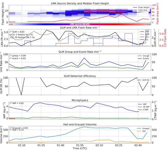
Figure 3.1: Timeseries plot of a thunderstorm that occurred on 20190701 near Cheyenne, WY. The top plot features the height of LMA VHF sources (km), median LMA flash height (km, black), and median LMA flash area (km2,red). The 2nd panel shows LMA and GLM flash rate (black and grey) in flashes per minute and +/- (red, blue) NLDN flash rates in flashes per five minutes. Notice that the GLM and LMA flash rates are on different scales. The third panel is a plot of GLM group and event products in units per minute. Panel 4 is the GLM detection efficiency in percent form. Panel 5 shows the ice water path (IWP, blue, kg m-2), above-flash ice water path (AF-IWP, green, kg m-2), and cloud-top water path (CTWP, red, kg m-2). The hail (orange) and graupel (blue) echo volumes of the storm are shown in panel 6 in km3. The x-axis of all panels is the time in UTC format. All correlation coefficient values in the upper-left portion of plots are relative to the LMA flash rate.
25
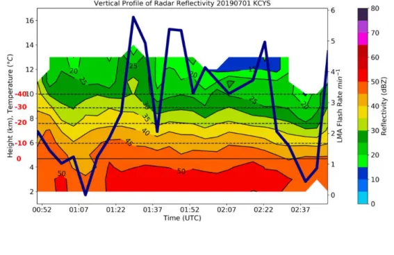
As discussed in Chapter 1, the collision of graupel undergoing riming with small ice crystals in the presence of supercooled liquid water results in significant electrification. Further exploration into the behavior of this thunderstorm is shown by the time height plot of radar reflectivity shown in Figure 3.2.
Figure 3.2: Timeseries plot of the 90th percentile of radar reflectivity (dBZ) with height (km) from a storm that occurred near Cheyenne, WY on 20190701. The radar reflectivity values are contoured every 5 dBZ. The temperature taken from the nearest sounding is plotted on the y-axis in degrees Celsius. The LMA flash rate is shown in Navy and is in units of flashes per minute.
The 40 dBZ contour resides in the mixed layer for the entire duration of this thunderstorm. The presence of the 40 dBZ contour above the 0 C line correlates to a high probability of lightning (Lang et al. 2011). One might expect this reflectivity profile to produce higher flash rates than a peak of 6 flashes min-1, but this is not necessarily the case. The vertical
reflectivity structure of Colorado thunderstorms is different than those in other parts of the United States (Fuchs et al. 2015, Rutledge et al. 2020). Colorado thunderstorms often boast increased reflectivity values in the mixed phase region. Therefore, this reflectivity structure is
26
towards the low-end of the intensity spectrum compared to the other Colorado storms that are discussed in this study.
The reflectivity structure of this thunderstorm is directly related to the IWP, hail, and graupel volumes. All of these values are relatively small for the duration of this thunderstorm (panels 5 and 6 of Fig. 3.1). The microphysics of the thunderstorm are likely related to the CTWP as well. This thunderstorm occurs at nighttime, so the CTWP (which is based on solar reflectance measurements) cannot be computed. However, due to the elevated flash heights (based on the VHF source location) the above-cloud portion of the CWP is likely to be small, and thus not playing a large role in attenuation optical energy detected by the GLM. However, it is likely the cloud water path is small which limits the scattering of the optical emissions
produced by lightning. The combination of high VHF source location, relatively large flashes, and increased GLM detection at night result in a high detection efficiency from GOES-17 GLM. 3.2.2 May 26, 2019
The next case is a moderate flash rate thunderstorm that occurred in Colorado during the afternoon of 26 May 2019. The timeseries of this thunderstorm is shown in Figure 3.3. This thunderstorm is much like the July 1st case except with moderately higher LMA flash rates. The
VHF source locations are once again relatively high in this thunderstorm—around 10 km— indicative of a normal polarity thunderstorm, but the LMA flash areas are mainly below 10 km2.
One feature of note is the occurrence of an overshooting top at 2200 UTC (MacGorman et al. 2017) and an apparent increase of the GLM products in the minutes following. Panel 2 of Fig. 3.3 shows that the LMA flash rate is an order of magnitude higher than the GOES-17 GLM flash rate for much of the event. Another indication that this storm is of normal polarity is that 90% of the CG flashes are of negative polarity. Negative polarity CG flashes represent 90% of all CG
27
flashes in the United States and are indicative of thunderstorms with normal charge structures (Williams et al. 1989, Boccipio et al. 2001). The GLM group and event rates have a high correlation to the LMA flash rate but the values smaller relative to the magnitude of the LMA flash rate. The difference in magnitude between the LMA flash rate and the GLM products is a result of GLM “missing” some of the flashes that are occurring in the thunderstorm. Most of the
28 flashes in this
Figure 3.3 Same as figure 3.1 but for a thunderstorm near Cheyenne, WY on 20190526. Notice that the GLM and LMA observations are on different scales in panel 2.
thunderstorm have an area of less than 10 km2 and thus the optical intensities of these flashes are
small compared to larger flashes. Previous studies have shown that GLM has a reduced detection efficiency for small flashes with low optical intensities (Zhang and Cummins 2020) and the
29
small flashes are the likely culprit for the reduced GLM DE in this case. The fifth panel reveals a large difference between the July 1st high DE storm and the present case. The microphysics of
this thunderstorm are more robust than the July 1st case. A more detailed structure of this
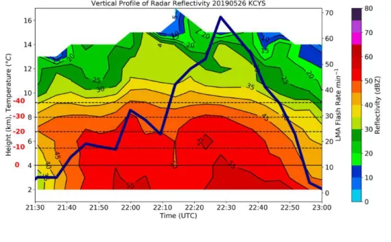
thunderstorm is shown in figure 3.4.
Figure 3.4: Same as Figure 3.2 but for a thunderstorm that occurred near Cheyenne, WY on 20190526.
The difference between this thunderstorm and the 1 July case is striking. The 50 dBZ contour breaches the freezing level for around 1 hour of this storm’s duration. The 55 dBZ contour breaches the freezing level near 22:25 UTC and shortly after this the thunderstorm records its highest LMA flash rate near 70 flashes per minute. It is also interesting to see that the LMA flash rate decreases significantly as the height of the 50 dBZ contour decreases. Indeed, the LMA flash rate is almost 0 by the end of the event where the height of the 50 dBZ contour is no longer above the freezing level. Additionally, since this thunderstorm occurred during the day, the CTWP is plotted in panel 5 of figure 3.3 and shows many values near 1 kg m-2, which we will
30
combination of small flash areas, increased cloud ice/water paths, and the reduced DE of GLM during the daytime result in a very low detection efficiency from GOES-17 GLM.
3.2.3 May 26, 2019 Anomalous Polarity Thunderstorm
The final Colorado thunderstorm presented occurred on the afternoon of May 26th, 2019.
The timeseries of this thunderstorm is shown in Figure 3.5. Unlike the previous storm from May 26th, the focus of VHF sources is low in altitude relative to the first two Colorado thunderstorms
presented (top panel). Many of the sources are located around 5-7 km, in contrast to the 9-10 km height of the previous cases. It is thus likely that this is an anomalous charge structure
thunderstorm with a mid-level positive charge layer (Fuchs et al. 2015, Fuchs and Rutledge 2018, Fuchs et al. 2018).
Panel 2 of Fig. 3.5 shows a large discrepancy between the COLMA flash rate and the GOES-16 GLM flash rate. The LMA flash rate peaks at ~250 flashes min-1 at 0020 UTC while
the GLM flash rate is almost two orders of magnitude less. The GLM group products do not reach 200 units per minute, but the event product is of a similar magnitude to the LMA flash rate. Panel two also shows that that the percentage of positive and negative CG strikes are almost even. The storm is dominated by +CG strikes from 2248 to 2318 UTC. After this period the storm produces equal amounts of +CG/-CG strikes from 2318 to 0018 UTC. Finally, the thunderstorm is dominated by -CG strikes for the remainder of its lifetime. The increased presence of -CG strikes from 0018 to 0050 UTC is curious, because the VHF source location at this time is located around 5-6 km. One would expect a high percentage of +CG strikes during this timeframe due to the evidence of a mid-layer positive charge which have been known to produce a high percentage of +CG strikes (Boccippio et al. 2001; Carey et al. 2003; Williams et al. 2005; Fuchs et al. 2015). It is clear that more research into the behavior of these
31
thunderstorms is needed. Another interesting feature of this figure is the increase in GLM event/group/flash rate associated with an increase in flash areal size near 2340 UTC. The larger flash sizes exhibit longer durations and more flash energy making them easier for GLM to detect.
Figure 3.5: Same as figure 3.1 but for a storm that occurred near Cheyenne, WY on 20190526. Notice that the GLM and LMA observations are on different scales in panel 2.
32
A time height plot of radar reflectivity of the May 26th thunderstorm is shown in Figure
3.6. The reflectivity structure of this thunderstorm is impressive. The 35 dBZ height stays at or above 10 km for the duration of the timeseries. Additionally, 50 dBZ contour resides in the mixed phase region (0 to -40 C) for the entire duration of the event. This thunderstorm produced very large hail reports of 2.50 and 3 inches in Weld County, Colorado. Large hail reports are very common in thunderstorms that produce a large percentage of +CG strikes (Boccippio et al. 2001; Carey et al. 2003).
Figure 3.6: Same as figure 3.2 but for a storm near Cheyenne, WY on 20190526.
The reflectivity values of this thunderstorm are more robust compared to the high Colorado DE case. Since graupel echo volumes are correlated to flash rate (Weins et al. 2005) we can infer that this thunderstorm will have a higher flash rate. This is actually something we can
demonstrate because of the LMA observations. The larger graupel volumes do indeed result in LMA flash rates of ~ 250 flashes min-1 at 0020 UTC. Additionally, the presence of larger hail
33
Increased SCLW contents can flip the polarity of charge on graupel in the mid-levels from negative to positive (Takahashi 1978). This change in the sign of charge imparted to graupel leads to anomalous charge structure thunderstorms like the one featured here. The anomalous charge structure thunderstorm in this case has higher values of reflectivity in the mixed phase region compared to the Alabama case studies. Thunderstorms in the Colorado region typically have increased reflectivity values and lower flash heights, both of which are characteristic of anomalous charge structure thunderstorms (Fuchs et al. 2015, Fuchs and Rutledge 2018, Fuchs et al. 2018). The low flash heights in this thunderstorm result in a very low GLM detection
efficiency from GOES-16 (Rutledge et al. 2020). 3.3 WEST TEXAS CASE STUDIES
3.3.1 April 23, 2019
Three West Texas cases are presented in this section ordered by highest to lowest GLM detection efficiency. The first case shown in the West Texas region is a very low flash rate storm that occurred on the night of April 23rd, 2019 and is shown in Figure 3.7. The top panel portrays
some interesting behavior from this thunderstorm. The majority of VHF sources in this
thunderstorm are located near and below 5 km. The low VHF source location might be due to the fact that this is weak thunderstorm with limited vertical extent. The vertical profile of radar reflectivity of this thunderstorm is shown in Figure 3.8.
The first feature of interest is that the 35 dBZ contour only breaches the -10 C level around 0135 UTC and is around 5 km at that time. Compare this to Figure 3.6 of the 20190526 anomalous charge structure Colorado thunderstorm, where the 35 dBZ contour extended to 12 km and the 50 dBZ contour overlays a large portion of the mixed phase region. Therefore, it is
34
likely that most of the electrical activity would be below the -10 C level, which is likely the reason for the low VHF source location. It is also noteworthy that the LMA flash areas are mostly greater than 50 km2 for the majority of the thunderstorm lifetime.
The 2nd panel of Figure 3.7 shows a low LMA and GLM flash rate, but a moderate -CG flash
rate of greater than 20 flashes per five minutes. If we assume that the LMA flash rate is a measure of the total lightning in the thunderstorm, then we can approximate the CG/IC ratio. There was a total of 188 LMA flashes recorded by the WTXLMA and a total of 167 CG flashes recorded by NLDN. Therefore, using this assumption, nearly 89 percent of the flashes from this thunderstorm were CG strikes. The combination of low VHF source location, large flash sizes,
35
and moderate -CG flash rate points to the probability that
Figure 3.7: Same as Figure 3.1 but for a thunderstorm near Lubbock, TX on 20190423.Notice that the GLM and LMA flash rates are on different axes in panel 2.
36
Figure 3.8: Same as figure 3.2 but for a thunderstorm near Lubbock, TX on 20190423.
this thunderstorm produced mostly cloud-to-ground lightning flashes. Panels 2 and 3 show a high correlation between the LMA flash rate and the GLM flash, group, and event products. Panel 5 shows very small ice water paths due to the weak instability that this thunderstorm formed in. Altogether, the GOES-16 GLM had a high detection efficiency of this storm because of large flash areas and a low IC/CG ratio (especially near 01:55 UTC). The higher DE follows from CGs having significant optical intensities which are then more readily detectable by an optical sensor such as GLM (Zhang and Cummins 2020).
3.3.2 May 5, 2019
The second West Texas case occurred on May 5th, 2019. This storm is also a relatively
low flash rate thunderstorm (Figure 3.9). A main feature of this thunderstorm is the location of VHF sources near 10 km, shown in Panel 1. This elevated source is indicative of a normal charge structure thunderstorm (Williams et al. 1985, Fuchs et al. 2015, Fuchs et al. 2016, Fuchs et al.
37
2018, Rutledge et al. 2020). Indeed, Panel 2 shows that this particular storm produced only 16 CG flashes, all of which were of negative polarity. This thunderstorm produced LMA flash rates below 10 flashes per minute until 21:14 UTC. The flash size is relatively large between 2024 and 2114 UTC which likely allows for a GLM detection efficiency that approaches 50%. However, the GLM detection efficiency drops below 20% at 2114 UTC when the LMA flash rate increases
38
above 20 flashes per minute and the LMA flash areas decrease to < 10 km2.
Figure 3.9: Same as figure 3.1 but for a thunderstorm near Lubbock, TX on 20190505.
The increase in VHF source activity is collocated with an increase in IWP around 2130 UTC as well as an increase in hail and graupel echo volumes. This behavior is consistent with non-inductive charging theory. A more detailed look into the reflectivity structure of this
39 thunderstorm is shown in Figure 3.10.
Figure 3.10: Same as Figure 3.2 but for a thunderstorm near Lubbock, TX on 20190505.
Figure 3.10 shows moderate reflectivity values in the mixed phase region from 2024 UTC to 2114 UTC. However, between 2114 and 2124 UTC, the 45 dBZ contour increases from around 3 km to nearly 12 km in height. This corresponds to an increase in the LMA flash rate from around 5 flashes per minute to a peak LMA flash rate of 25 flashes per minute. Additionally, values of 50 dBZ were also present in the mixed phase region at the time of the peak LMA flash rate. The 20190505 west Texas case is a great example of thunderstorm electrification via the
non-induction charging method (Reynolds et al. 1957; Takahashi,1978; Jayaratne et al. 1983; Baker et al. 1987; Saunders et al. 1991). The increase in reflectivity is correlated to an increase in graupel concentration and likely supercooled liquid water content in the mixed phase region. Therefore, more increased collisions between ice crystals and graupel are probable, which results in increased electrification shown near 2124 UTC. This is an example of a thunderstorm that produced large flash areas in the early stage with a moderate detection efficiency by GLM.
40
However, as the flash rate increased after 2114 UTC with associated smaller flash areas, the GLM DE decreased.
3.3.3 June 24, 2019
The final West Texas storm to be described occurred on the evening of June 24th, 2019.
This thunderstorm was a high flash rate thunderstorm that produced flash rates in excess of 200 flashes per minute (Figure 3.11). The top panel shows that the location of the VHF sources is near 10 km and that the LMA flash areas are very small with an average size less than 10 km2.
The second panel shows that this thunderstorm was electrically active with LMA flash rates over 100 flashes min-1 for over an hour of the storm and a total of 498 CG strikes occurring during the
duration of the storm. It is worth noting that almost 90% of these flashes were of negative polarity, which is typical of normal polarity thunderstorms which frequent this area (Williams et al. 1985, Fuchs et al. 2015, Fuchs et al. 2016, Fuchs et al. 2018, Rutledge et al. 2020).
The GLM flash rate has a significant correlation to the LMA FR but the GLM flash rate is an order of magnitude less. Apparently, many of small LMA-detected flashes are below the detection threshold of the GLM CCD. The graupel volume within this thunderstorm shown in Panel 6 reached a maximum near 0125 UTC which is generally where the peak of the LMA flash
41
rate occurs. The reflectivity structure of this thunderstorm is shown in Figure 3.12.
42
Figure 3.12: Same as figure 3.2 but for a storm near Lubbock, TX on 20190625.
Figure 3.12 shows that the height of the 35 dBZ contour is above 14 km from 0114 UTC to 0200 UTC. This is the likely reason for VHF sources near 13-14 km shown in panel 1 of Figure 3.11. It is interesting to note that the only presence of the 55 dBZ contour in the mixed phase region occurs at 0114 UTC. This is also the time of the peak LMA flash rate > 200 flashes per minute in this thunderstorm. The IWP, hail, and graupel volumes are also at near maximums at 0114 UTC. Once again, the combination of increased reflectivity values and graupel is
evidence for the NIC method for thunderstorm. The lightning flash rate of this thunderstorm begins to decrease ~0200 UTC coincident with the decrease in height of the 45 dBZ contour. After a slight increase in reflectivity values at 0229 UTC, the height of the 40 dBZ contour decreases below the 0 C level and the LMA flash rate decreases almost to 0 flashes per minute. This behavior is consistent with Lang et al. 2011 which showed that the 40 dBZ contour above the 0 C level is a sufficient requirement for lighting in convection.
43
This is the type of thunderstorm that GLM has the most difficulty in characterizing. The combination of extremely small flash sizes, consistent with reduced optical intensities (Zhang and Cummins 2020) and the likelihood of increased above-flash cloud water/ice path result in a severely reduced detection efficiency from GLM.
3.4 ALABAMA CASE STUDIES
3.4.1 MAY, 17 2020
The first Alabama case shown occurred on 17 May 2020. This case had the highest average GLM detection efficiency of any thunderstorm in this study at 59%. The timeseries of this storm is shown in Figure 3.13. The top panel of Figure 3.13 shows that positive charge region of this thunderstorm was located primarily around 10 km and that the flash areas were generally larger than 10 km2 for the duration of the thunderstorm. The 2nd panel shows that the
LMA and GLM flash rates are highly correlated and that the GLM flash rate has a similar magnitude to the LMA flash rate. Additionally, Panel 2 shows that 90 out of 105 CG flashes in this storm were of negative polarity, which is characteristic of a thunderstorm with a normal charge structure. Panel 5 shows reduced IWP, AF-IWP, and CTWP values for this Alabama thunderstorm, in comparison to previous cases. In fact, the AF-IWP is close to 0 kg m-2 which is
likely evidence of weak updrafts in the mixed-phase region of this thunderstorm, unable to loft significant amounts of graupel. The CTWP is barely above 0 kg m-2 which is substantially
smaller in comparison to the previous cases.
If we compare this case to the 26 May 2019 Colorado thunderstorm shown in Figure 3.6, we see some extreme differences. First, the AF-IWP in the Colorado case approaches 5 kg m-2
44
graupel volume in the Colorado case achieves peak values in excess of 5000 km3 while the
Alabama storm only produces values near 250 km3.
Figure 3.13: Same as figure 3.1 but for a thunderstorm near Huntsville, AL on 20200517.Notice that the GLM and LMA flash rates are on different axes in panel 2.
The vertical profile of radar reflectivity is shown in Figure 3.14. There are modest reflectivity values in the mixed phase region for the duration of this thunderstorm. One
45
interesting feature of this plot is the increasing in lightning that occurs after the 50 dBZ contour breaches the 0 C level at 1950 UTC and 2020 UTC.
Figure 3.14: Same as figure 3.2 but for a thunderstorm near Huntsville, AL on 20200517.
In fact, this thunderstorm reaches its peak flash rate of ~20 flashes per minute about 10 minutes after the 50 dBZ contour approached the -10 C level. Once again, the lightning nearly ceases in this thunderstorm once the height of the 40 dBZ contour falls below the mixed phase region. The reduced microphysics, combined with the relatively large flash areas, result in a GLM DE that is close to the specification value of 70%.
3.4.2 JULY 4, 2020
The next case presented occurred on the afternoon of Independence Day in 2020 and is shown in Figure 3.15. This case is of particular interest because of the dynamic nature of the GLM detection efficiency shown in Panel 4 of Figure 3.15. The GLM DE decreases to a few percent near 1810 UTC before increasing close to 70% near 1820 UTC and stays above 50% for
46
the majority of the storm after that time. Notice that the lowest GLM DE is co-located with a time period of extremely small flash areas (< 10 km2) from 1750-1810 UTC. These very small
flashes with reduced optical intensities (Zhang and Cummins 2020) appear to be difficult for
Figure 3.15: Same as figure 3.1 but for a storm near Huntsville, AL on 20200704. Notice that the GLM and LMA flash rates are on different axes in panel 2.
GLM to detect, especially during an afternoon storm such as this one. Flash area increases significantly after 1810 UTC which leads to a local maximum of the GLM flash rate close to
47
1815 UTC (Panel 2). Between 1815 and 1830 UTC the flash rates from GLM, LMA, and NLDN decrease to only a few flashes per minute corresponding with decreased microphysics (Panels 4 and 5) indicating the storm has weakened. Starting at 1835 UTC the VHF source activity increases, reaching its highest value (Panel 1) and there is a corresponding increase in GLM, LMA, and NLDN flash rates. Notice that some of the highest GLM detection efficiencies are correlated with the maximum in NLDN CG- flashes. These flashes are longer in duration and size, which allow the GOES-16 GLM a better chance at detection.
It is interesting to note that the CTWP in this case (Panel 5) is much higher than the May 17th, 2020 case (figure 3.13), suggesting reduced DE due to cloud scattering (Brunner and Bitzer
2020). However, the difference between the two cases is the larger flash areas in the July 4th case
compared to the May 17th case. The vertical profile of reflectivity for this thunderstorm is shown
in Figure 3.16.
48
This thunderstorm included increased in lightning at 1808 UTC and ~1835 UTC. Interestingly, the first increase in lightning is not coincident with increases in hail or graupel volume (Figure 3.15, Panel 6). However, this increase in electrical activity is correlated with an increase in IWP and the presence of the 50 dBZ contour. The second increase in lightning activity is coincident with an increased graupel volume, presence of the 50 dBZ contour, and increased IWP. The CTWP also increases around this time. The larger flash areas result in brighter optical intensities which GLM is likely to detect despite the increased CTWP.
3.4.3 8 April 2020
The final Alabama case occurred on the afternoon of April 8th, 2020. The timeseries of
this thunderstorm is shown in Figure 3.17. This case is interesting because the height of the VHF sources decreases throughout the storm’s duration (Panel 1). At the beginning of the storm, the height of the VHF sources is located near 10 km. However, near the end of the thunderstorm’s lifetime, the location of VHF sources is ~6 km.
The location of positive charge lower in the cloud (Panel 1) and the increased
concentration of +CG strikes (Panel 2) suggests that this could be an end of storm oscillation (Marshal and Lin 1992; Williams et al. 1994; Pawar and Kamra 2007; Marshal et al. 2009). EOSO’s occur near the decaying stages of thunderstorms where the mid-level negative charge region begins to decay (or falls out in the form of precipitation), and the upper positive charge settles to lower altitudes (Marshal and Lin 1992; Williams et al. 1994; Pawar and Kamra 2007; Marshal et al. 2009). At this time, the thunderstorm can produce +CG strikes before its decay.
The end of storm oscillation phenomenon appears to be at play in this case. The LMA flash rate peaks at > 100 flashes per minutes at ~2220 UTC and ~2315 UTC. The GLM flash, group and event rate peak about 5 minutes after the initial peak in LMA flash rate at 2220 UTC.
49
The GLM flash rate only reaches a value of 25 flashes per minute at this time, but the GLM group and event products are both higher than the LMA flash rate. One factor that is apparent in this case is the variation of GLM DE with region. If we compare this to the anomalous charge structure 20190526 CO thunderstorm, the behavior of GLM is different. The Alabama storm has
50
LMA flash rates that peak over 100 flashes per minute twice, while the
Figure 3.17: Same as figure 3.1 but for a thunderstorm near Huntsville, AL on 20200408. Notice that the GLM and LMA flash rates are on different axes in panel 2..
Colorado thunderstorm had LMA flash rates that peak over 200 flashes per minute ~3 times. The GLM flash rate in the Alabama storms increases over 25 flashes per minute both times the LMA flash rate peaks. However, the GLM flash rate only rises above 20 flashes per minute one time
51
when the LMA flash rate is well over 200 flashes per minute. This is a great example of the degradation of GLM DE with increasing distance from nadir (Cummins 2020). Thunderstorms in the Alabama region are close to the GOES-16 satellite nadir and therefore the optical brightness required for a flash to be “seen” is low (Cummins 2020). However, the brightness threshold in Colorado is higher due to the increased distance from GOES-16 and GOES-17. GLM aboard GOES-17 missed out on numerous optically dim flashes that occurred in the 20190526 Colorado storm, but more of these same flashes were likely detected in the Alabama thunderstorm due to the difference in brightness threshold.
Another aspect of this thunderstorm that requires more analysis is the vertical profile of radar reflectivity shown in Figure 3.18.
Figure 3.18 highlights the two major peaks in LMA flash rate occurring around 2220 UTC and 2315 UTC. The first increase in LMA flash rate is coincident with an increase of reflectivity values in the mixed phase region. Once again, the 50 dBZ contour breaching the 0 C degree levels occurs during the time of the highest flash rate. The IWP of this storm (Figure 3.17, Panel
52
5) also reaches a maximum at this point, but the hail and graupel volumes are consistent. The second peak in LMA flash rate is also coincident with an increase in reflectivity values in the mixed phase region as well as increases in IWP and graupel volume. This is an example of a high flash rate thunderstorm in Alabama. All of the same issues that cause decreased GLM DE are there such as relatively small flash areas and increased microphysics in the mixed phased region. However, in this case, some of that is overcome due to Alabama’s close proximity to the nadir of GOES-16.
3.5 SUMMARY OF CASE STUDIES
Section 3 featured case studies of thunderstorm from the Colorado, West Texas, and Alabama regions. In all three regimes, GLM struggled to detect lightning in thunderstorms compared to the LMAs. While there is no golden standard for every storm, there were similarities in the lightning and microphysical characteristics of the thunderstorms and the resulting GLM detection efficiencies. The first detail to note is that the GLM DE efficiency was high only when thunderstorms had a low LMA flash rate. The second aspect is that the presence of small lighting flash areas often results in a low GLM detection efficiency. These small flashes correspond to reduced optical intensities (Zhang and Cummins 2020) which limits detection by GLM. Indeed, there were examples from the case studies where the LMA flash size temporarily increased which led to a local maximum in the GLM flash products and DE.
The final detail to focus on revolves around the microphysics of the thunderstorm case studies. Thunderstorms with a higher CTWP are more likely to have lower detection efficiencies. In thunderstorms with increased above-flash cloud ice/water paths, the “mean free path” (or the path in which a photon would encounter a cloud particle) is very small. Thus, a photon is more likely to be backscattered or scattered out of the sides of the cloud than it is to escape the top of
53
the cloud in the line-of-sight of GLM. This effect also leads to a decreased detection efficiency from GLM. Chapter 4 will provide statistical plots from all of the case studies to further
54
CHAPTER 4: STATISTICAL RESULTS
In this chapter we synthesize results from numerous convective cells by presenting and discussing a series of statistical plots to further underpin the processes that contribute to GLM detection efficiency. This section provides further clarity by leveraging the large number of lightning flashes that were documented in this study. Only data from within the CLEAR tracked 35 dBZ contour and within 100 km of the LMA center were considered in this study.
One storm cell from each case was chosen for an in-depth time series analysis some of which are shown in Chapter 3. Table 4.1 provides a list of 34 thunderstorms from each case with the date, region, time of cell observation, SPC hail, wind, and tornado reports, and the average GOES-16 GLM detection efficiency. The first main detail of this table is that many of these cases had a low average GLM detection efficiency. Some of the cases in Chapter 3 show that the detection efficiency of GLM significantly decreases when the LMA flash rate is large. This finding will be further explored in this chapter.
The next key aspect of this table is the fact that thunderstorms with lowest GLM DE (< 10%) were more likely to be associated with a SPC severe weather report. The most frequently reported severe weather category was hail. This is a significant result because one of the stated goals of GLM was to help with the detection of severe weather reports by detecting rapid increases in the production of lightning termed the lightning jump (Schultz et al. 2015). There were several cases shown in Chapter 3 where there is a very small dynamic range in GLM flash rate. While this study did not evaluate lightning jumps in the cases directly, by inspection of Figs. 3.1-3.18 we can see that that there is often little to no dynamic range in the GLM flash