The Halloween
Effect
MASTER THESIS WITHIN: Business Administration, Finance NUMBER OF CREDITS: 30
PROGRAMME OF STUDY: Civilekonom
AUTHOR: Oliver Benjaminsson and Pontus Reinhold TUTOR: Fredrik Hansen and Toni Duras
JÖNKÖPING May 2020
Master Thesis in Business Administration, Finance
Title: The Halloween effect
Author: Oliver Benjaminsson and Pontus Reinhold Tutor: Fredrik Hansen and Toni Duras
Date: May 2020
Key Terms: The Halloween Effect, Efficient Market Hypothesis, Calendar anomalies, Regression analysis, Trading strategies
Abstract
The Halloween effect refers to higher stock returns during the period November to April compared to May to October. This is a well-known calendar anomaly that has gained a lot of attention due to the fact that the effect is persistent in the market in spite of the fact that investors are aware of the anomaly today. This evokes questions regarding the efficiency in the markets and the Efficient Market Hypothesis in particular. The main focus of this thesis was to investigate whether the Halloween effect still exists in the Swedish stock market and if the power of the effect deviates between different firm sizes. Furthermore, we examined risk differences between the summer -and the winter months, as well as the January effect in order to find out if these could be possible explanations for the Halloween effect and its existence. A trading strategy based on the Halloween effect was also tested in order to see if investors could use this strategy to outperform a buy and hold strategy. The method that was used to investigate the existence of the Halloween effect was Ordinary Least Squares regression models with dummy variables, standard deviation to ascertain risk-differences between the periods and the Sharpe ratio to determine the risk-adjusted returns of the trading strategies. The results showed that the Halloween effect could be found in all of the examined market-cap indices, and therefore the Efficient Market Hypothesis could be questioned. The Halloween effect turned out to be autonomous from the January effect and the risk measured in standard deviation had no significant difference between the summer -and the winter months, hence, both these possible explanations were rejected. The backtesting showed that the Halloween strategy would perform better than the buy and hold strategy in all indices except from the mid-cap index. The results regarding the Sharpe ratio indicated that the Halloween strategy would be a better strategy to use considering risk-adjusted returns as the Sharpe ratio was higher in all indices.
Acknowledgements
We would like to pay our special regards and deepest gratitude to our tutors. First of all, Fredrik Hansen for his monumental guidance and advice during this thesis. Second of all, Toni Duras for his invaluable help in making sure the statistics in this study is made in the best and most efficient way possible. We would also like to show our gratitude to the other students that have participated in the seminars, providing us with useful opinions and suggestions.
Oliver Benjaminsson Pontus Reinhold
Jönköping International Business School May 2020
Table of Contents
1
Introduction ... 1
1.1 Background ... 1 1.2 Problem Discussion ... 3 1.3 Purpose ... 5 1.4 Delimitation ... 5 1.5 Definitions ... 62
Literature Review ... 7
2.1 The Efficient Market Hypothesis and Anomalies ... 7
2.2 The January Effect ... 8
2.3 The Halloween Effect ... 10
2.3.1 Possible Explanations for the Halloween effect ... 11
2.3.2 The Halloween Effect and The January Effect ... 12
2.3.3 Risk ... 13
2.3.4 The Halloween Effect from 2015 and After ... 14
2.4 The Halloween Effect as a Trading Strategy ... 15
2.4.1 The Sharpe Ratio ... 16
3
Methodology ... 17
3.1 Research Strategy ... 17
3.1.1 Methodological Assumptions ... 18
3.2 Data Collection ... 19
3.3 Reflections on the Chosen Data ... 20
3.4 Statistical Methodology ... 21
3.4.1 Hypothesis Testing ... 24
3.4.2 Heteroscedasticity and Autocorrelation ... 25
3.5 Economic Significance and Trading Strategy Implications ... 26
4
Results / Empirical Findings ... 28
4.1 The Halloween Effect in the General Market ... 28
4.2 The Halloween Effect in the Different Firm Sizes ... 29
4.3 The Halloween Effect as a Trading Strategy ... 31
5
Analysis ... 38
6
Conclusion ... 42
7
Discussion and Further Research ... 44
8
References ... 47
8.1 Internet References ... 50
1
Introduction
In the introduction chapter of this thesis, the background of the subject is presented. Thereafter, we discuss the problem as well as state the purpose of this thesis. In the later stage of the introductory part, one can find some practical headlines including definitions and delimitations that is necessary to understand to follow this thesis.
1.1
Background
“Sell in May and Go Away” is an old saying as well as a trading strategy that goes as far back as 1697. The expression refers to that May is the start of a period with lower returns, and therefore investors are better off by selling all of their holdings in the market and hold cash over the summer. When investors enter the market again after the summer differs depending on what type of strategy the investors are using. The “Sell in May and Go Away”-expression has two different endings, one is “but remember to come back in September” and another one is “but buy back on St. Leger Day”, which refers to a horse race that takes place in England every mid-September (Bouman and Jacobsen, 2002). Another concept for the same phenomenon is known as the “Halloween indicator” or the “Halloween effect”, which is another saying that was introduced by O’Higgins and Downes (1990) and suggests that the investor should come back into the market in the start of November, hence dividing the year in to six summer months and six winter months.
A seminal study made by Bouman and Jacobsen (2002) examined whether the Halloween effect was present in several stock markets all over the world. Their study examined 37 countries and compared the returns for the period May to October and the period November to April for each country. The number of years that they tested differed depending on what country they investigated, as the data availability was limited in some countries. For most of the developed countries, they used value-weighted market indices and tested the effect between January 1970 to August 1998. What Bouman and Jacobsen found was that the difference in returns was significant, especially in Europe, where the average return in the summer months did not exceed 2 percent for any country except Denmark. This can be compared with the winter months where the average return exceeded 8 percent in all countries. In total, the Halloween effect could be seen in all 37
countries except New Zealand. The findings of Bouman and Jacobsen’s research has in more recent years been confirmed in several studies; Andrade et al., (2013), Degenhardt and Auer, (2018), Jacobsen and Visaltanachoti, (2009).
The Halloween effect is one of several anomalies in the stock market. Anomalies are inconsistencies or something that deviates from the classical asset-pricing theories and that can create opportunities for investors (Schwert, 2003). These phenomena question the Efficient Market Hypothesis (EMH), which states that in an efficient market, investors should not be able to gain advantages from publicly available information (Fama, 1970). If an anomaly appears in the market that creates opportunities for investors, the opportunity will diminish over time as the strategy becomes identified by investors (Jensen, 1978). What is interesting to note, is that calendar-related anomalies such as the January effect, the holiday effect and the time-of-the-month effect, according to Marquering, et al. (2006), disappears as soon as they are “revealed” or known to the market, which is in line with the EMH. According to their study, this is due to that investors become aware of these anomalies and start to trade based on them. However, the Halloween effect has been a well-known anomaly for many years and it has not disappeared completely, as other anomalies normally do (Bouman and Jacobsen, 2002). Researchers within this field have not concluded a shared concrete explanation for the existence of the Halloween effect. Bouman and Jacobsen (2002) examined some possible explanations such as data mining, risk differences, liquidity and length and time of vacations. However, they were only able to prove that the time and length of vacations were statistically significant and rejected the other suggestions. Bouman and Jacobsen also investigated whether the January effect could explain the presence of the Halloween effect. The January effect is also a recognized calendar anomaly that suggests that January yields an extraordinary return compared with the other months, presented as early as 1942 by Wachtel (1942). The month of January is included in the winter months, which questions if the Halloween effect is driven by high returns in January. Therefore, the January effect as a possible explanation for the Halloween effect has been reported in several studies; Haggard and Witte (2010), Lucey and Zhao (2008). Jacobsen and Visaltanachoti (2009) thoroughly examined whether the magnitude of the Halloween effect could vary depending on sectors. Their results suggested that consumer sectors tend
to perform better during the summer whilst the production sector tends to perform better during the winter.
In research concerning the Halloween effect, there is to our understanding no previous studies that covers the market capitalization of firms and if the strength of the Halloween effect deviates between different firm sizes. Therefore, the authors of this thesis have decided to investigate this in the Swedish stock market. By doing so, this thesis will provide new insights into the puzzle of the Halloween effect and its persistence by analyzing it from an innovative perspective. Our intention is to evoke new aspects of the effect and its possible explanations that later can be analyzed and examined further in future research.
1.2
Problem Discussion
Previous studies on the Halloween effect have provided clear evidence for the effect in several markets worldwide, first proven by Bouman and Jacobsen (2002). According to Fama (1970), seasonal effects should not appear over longer periods of time. Therefore, if this study shows that investors still can take advantage of this calendar anomaly, Fama’s hypothesis is questioned. This thesis aims to examine if the Halloween effect still exists in the market after the publication of Bouman and Jacobsen’s (2002) study and due to the fact that anomalies tends to diminish over time. Their research covered the period between 1970 to 1998 and it was released to the public in 2002. Hence, this thesis will provide an up-to-date study on the Halloween effect and investigate if the effect has weakened or disappeared after the publication of Bouman and Jacobsen’s study. The time period that will be tested is hence 2003 to 2019 and the study will be made on the Swedish stock market. The statistical testing will consist of Ordinary Least Squares (OLS) regression models in order to assess whether the returns for the winter months are statistically different from the summer months.
The impact of the Halloween effect on different firm sizes has not been sufficiently explored by researchers within this area. To our understanding, the effect from a market capitalization perspective on the Swedish stock market has not previously been examined. The motive for why we find this aspect to deserve elaboration is due to the fact that previous research has examined the Halloween effect mostly by using value-weighted indices for different countries. This means that the return of the shares with the largest
weight in the index will make up for most of the result, hence the result can be misleading. By examining the Halloween effect on all stocks on the Swedish stock market using the index OMXSPI as well as three different market cap indices, one will get a comprehension of whether or not the effect is a market-wide phenomenon or if it is concentrated to particular firm sizes.
Previous studies have discussed the relationship between the Halloween effect and the January effect, however, the results diverge between studies and researchers suggest that further research is necessary. Since the month of January has been proven to yield an extraordinary return, the January effect could be an explanation for why the Halloween effect exists. Therefore, this study will include the January effect in the regression analysis in order to answer this question.
Another question that this thesis will try to answer is whether the excess return earned during the winter months is compensated by a higher level of risk in the market during those months. If that is the case, that could be an explanation for why the Halloween effect exists. The risk will be measured by looking at the standard deviation where we will compare this measure between the winter months and the summer months in order to find the answer to this question. This study will also investigate whether the Halloween effect can be used as an effective trading strategy that can offer trading opportunities for investors. In order to examine this, the total return of a buy and hold strategy will be compared with the total return of a strategy based on the Halloween effect. Besides this, the Sharpe ratio measurement will be used to determine if a Halloween strategy offers a higher risk-adjusted return compared with a buy and hold strategy.
The perspective that this thesis will be written from is the investors perspective. With investors we regard both private- and institutional investors that could benefit from knowing whether or not the Halloween effect exists in the Swedish stock market, and if it does, if one could use the effect as an efficient trading strategy.
1.3
Purpose
To recapture the above, the main objective of this thesis is to investigate if the Halloween effect still exists in the Swedish stock market and if the strength of the effect deviates between different firm sizes. In addition to this, we will first examine if the Halloween effect is driven by abnormal returns in the month of January, secondly, if the risk measured in standard deviation is higher during the winter months and therefore motivates higher returns during these months, and thirdly if the Halloween effect can be used as a trading strategy and challenge a buy and hold strategy.
1.4
Delimitation
This study will only focus on the Swedish stock market, which means that the results found in this study only can be thought of as true in this market alone. However, this entitles other researchers to make future research on other markets to see if our results can be confirmed in the rest of the world’s stock markets.
Due to data limitations in the large cap index in Sweden, an alternative index is used and therefore all stocks are not covered in the analysis. The indices that are examined in this thesis are all price indices, which we chose to use as dividends are excluded. The motive for this is that most of the companies on the Stockholm Stock Exchange pay their dividends in the spring, which can be misleading as we aim to investigate seasonality in returns.
Moreover, we have decided to not include transaction costs in the testing. Bouman and Jacobsen (2002) mentioned that other anomalies usually can be explained by the simple fact that the cost of trading outweighs the potential economic benefits. However, they conclude that if one assumes reasonable transaction costs, the Halloween effect remains statistically significant. This is one of the reasons for why we chose to not include the transaction costs in our testing. Another reason is that a trading strategy based on the Halloween effect only requires the investor to pay transaction costs twice a year and that the transaction costs in later years has decreased significantly, therefore we assume that they would not have affected the result of this thesis.
1.5
Definitions
Price index (PI) - A price index means that the index does not include any types of dividends, hence the development of a price index is only due to price changes (Nasdaq, 2018).
OMXSPI – This index is being used as our general market index. The OMX Stockholm All-Share index consists of all 368 stocks listed on OMX Nordic Exchange Stockholm and it aims to reflect the overall development of the Swedish stock market. OMXSPI is a price index (PI) with base value 100 and base date December 31, 1995 (The Nasdaq Group, 2020a)
Large-cap index - The official name of this index is OMX Stockholm Large Cap PI (Symbol: OMXSLCPI) and it consists of all large-cap companies that are listed on the Stockholm Stock Exchange. The number of components is 129 and the base value is 100 (The Nasdaq Group, 2020b).
Mid-cap index - The index that we use as our mid-cap index is called OMX Stockholm Mid Cap PI (Symbol: OMXSMCPI). This index has 131 components and reflects the development of the mid-cap segment on the Swedish stock market. The base value is 100 (The Nasdaq Group, 2020c).
Small-cap index - The official name of this index is OMX Stockholm Small Cap PI (Symbol: OMXSSCPI) and it is compiled by The Nasdaq Group. The aim of this index is to represent and reflect the development of the 107 smallest companies listed on the Stockholm Stock Exchange. The base value of this index is 100 (The Nasdaq Group, 2020d).
OMXS30 - The OMX Stockholm 30 includes the 30 most traded stocks on the Stockholm Stock Exchange. This index is a market weighted price index and its composition is revised twice a year (The Nasdaq Group, 2020e)
Buy and hold strategy – A buy and hold strategy refers to a trading strategy that invests in securities once and the positions are held without doing any transactions during a longer period of time, thus minimizing transaction costs as well as tax expenditures (Nanda and Peters, 2006).
2
Literature Review
In the literature review, previous research is presented to give the reader a good overview and an understanding of the subject and key concepts. The structure of the literature review starts from a broader perspective with the underlying theories and ends up with the main topics of this thesis.
2.1
The Efficient Market Hypothesis and Anomalies
Eugene Fama laid the foundation for the current understanding of asset pricing with his famous publication in the Journal of Finance in 1970, in which he presented the most well-known study on the efficiency of capital markets and developed the Efficient Market Hypothesis (Fama, 1970). The EMH claims that market prices should reflect all available information. In the study, he considered the adjustments of security prices with respect to three different categories based on the nature of the information. Weak-form test refers to the information on past prices and trading volume, which is available to all investors. The semi-strong form includes all available information and the efficiency of the market to adjust prices when there are changes in the publicly available information. For instance, when firms announce earnings reports, stock splits, new security issues, etc. Finally, the study evaluates the strong-form, which means that all available information is accounted for in the market prices, including the monopolistic information that only insiders or other similar types of investors have access to. The study did not find any evidence against the hypothesis that prices should reflect all available information regarding the weak-form and semi-strong tests, and the strong-form test had limited evidence against the same hypothesis. Fama mentions that the statement that all available information “fully reflects” into the market prices and that markets therefore are efficient, is very general and that it is hard to interpret exactly what “fully reflects” really means (Fama, 1970 p. 384).
If markets really are efficient, investors should not be able to earn excess returns. Despite this, investors do find undervalued companies allowing them to earn excess returns Qianwei, et al. (2019). In their study, they investigated the possible explanations for why investors are able to earn excess returns. Anomalies are irregularities in returns that cannot be explained by any developed asset pricing theories, and these anomalies are found by investors allowing them to earn excess returns. However, research shows that
as soon as an anomaly is found in the market and documented in financial literature, i.e. become part of the public information, they seem to disappear or weaken, which is in line with the EMH. Furthermore, they conclude that investors do not always act rationally since they will make mistakes and misjudgments leading to opportunities for other investors to yield excess returns, both in short -and long term. Several studies have concluded that markets are in fact inefficient, at least not as efficient as proposed by Fama (1970). Instead, the reality of the EMH now exists in relative terms (Qianwei et al. 2019). Calendar anomalies are seasonal movements in stock prices that are related to a specific time period and they were first reported by Wachtel (1942). Lo (2004) has on the basis of these calendar anomalies developed an alternative hypothesis, called the Adaptive Markets Hypothesis (AMH). This alternative to the EMH allows the degree of efficiency of the markets to vary over time. Urquhart and McGroarty (2014) tested the Monday effect, January effect, turn-of-the-month effect and the Halloween effect, which all are well-known calendar anomalies, from January 1900 to December 2013 on Dow Jones Industrial Average in order to see if there were a pattern in the behavior of these calendar anomalies that can be connected to the AMH. Their study confirmed that these market anomalies do in fact vary over time and are more or less favorable depending on the market conditions, which is consistent with the AMH. They also examined different trading strategies based on calendar anomalies, which also deviates in efficiency depending on market conditions. These findings are consistent with the AMH but inconsistent with the EMH (Urquhart and McGroarty, 2014).
2.2
The January Effect
Similar to the Halloween effect, the January effect is a recognized calendar anomaly in the stock market. The origin of the January effect has emerged from abnormal stock returns during the month of January, and this phenomenon was first discussed by Wachtel (1942). The relationship between the Halloween effect and the January effect was investigated by Bouman and Jacobsen (2002) and has further been discussed in several studies: Haggard and Witte (2010), Lucey and Zhao (2008).
It was first mentioned by Wachtel (1942) that introduced the January effect in 1942, however, the first comprehensive study on the effect was made by Rozeff and Kinney (1976). Their study focused on the U.S. stock market where they examined aggregate
rates of return in an equally-weighted index for New York Stock Exchange (NYSE) from January 1904 to December 1974. In their calculations, they compared the average return for each month in order to investigate whether seasonality was present in any of the months. The results showed that January outperformed the other months over time, with an average monthly return of 3.48 percent. The average return for the remaining months was only .42 percent. Furthermore, Rozeff and Kinney (1976) provided clear evidence of an existing January effect in the U.S. stock market.
The size effect is another anomaly in the stock market, which suggests that there is a difference in risk-adjusted return between small-cap -and large-cap stocks. Evidence of the size effect in the American stock market was first reported by Banz (1981). In a study published by Keim (1983), an attempt to relate the size effect to the January effect on the U.S. market was introduced by examining the size effect on a month-to-month basis. The article examined the period 1963 to 1979 and provided clear evidence that the small-firm effect is to a large extent driven by abnormal returns in the month of January. These findings were also confirmed by Reinganum (1983).
Hypotheses that seek to explain the anomaly was not examined in the article by Rozeff and Kinney (1976), however, the study suggested that the tax-selling hypothesis deserved future elaboration. The tax-selling hypothesis as a potential explanation for the January effect was thoroughly discussed by Ritter (1988). The hypothesis relies upon that individual investors have an incentive to sell assets that have decreased in price before January, since the investors only can deduct losses that are realized, hence, their tax expenditures are reduced. In order for individual investors to reduce their tax expenditures, they sell their holdings during December and reinvest their funds in January. Their moneyis mainly invested in small stocks, which pushes the stock prices upwards for small-cap stocks in January. This finding goes in hand with previous studies that have suggested a relationship between the January effect and the size effect; Keim (1983), Reinganum (1983).
In a more recent study by Haug and Hirschey (2006), “window dressing” as a possible explanation for the January effect was investigated. The concept suggests that institutional investors seek to erase embarrassing losers in their portfolios before reporting periods. However, the researchers considered this explanation to be of poor
relevance for the January effect since “window dressing” mostly is related to institutional investors, which mainly invests in large-cap stocks. Furthermore, since the January effect is proven to be related to small-cap stocks, the explanation was then rejected. The research also examined value-weighted returns for Dow Jones Industrial Average for the period 1802 to 2004 in order to support previous evidence that has confirmed that the January effect is not persistent in large-cap stocks: Lakonishok and Smidt (1988). Haug and Hirschey’s (2006) results showed no tendency of higher returns in the month of January, which further confirmed that the January effect is not persistent in large-cap stocks or value-weighted indices. In their test for the equally-weighted index from the Center for Research in Security Prices (CRSP) that covered the period 1927 to 2004, their findings were consistent with previous studies on equally-weighted indices and further confirmed a strong January effect in small stocks (Haug and Hirschey, 2006).
2.3
The Halloween Effect
Bouman and Jacobsen (2002) provided the first comprehensive study on the Halloween effect where they investigated the effect in several countries. The main purpose of their study was to examine if the stock returns during the period May to October were significantly different from the period November to April. Their results showed that there was a substantially higher return during the winter months compared with the summer months, which indicated an existing Halloween effect. This effect could be found in 36 out of 37 countries, including Sweden. In their investigation, they used continuously compounded returns for the indices they examined. The data was retrieved from MSCI and their investigation analyzed the Halloween effect between 1970 to 1998. In addition to the results regarding average returns, Bouman and Jacobsen (2002) argued that it is of high importance to test if the effect is statistically significant. In their analysis, statistical significance for the Halloween effect could be seen in 20 out of the 37 countries. The result for Sweden indicated a strong Halloween effect as the statistical significance was high with a t-statistic equal to 3.32. The study of Bouman and Jacobsen (2002) was in 2013 followed up by Andrade et al. (2013). Their research was the first extensive out-of-sample analysis of the Halloween effect, which covered the same countries as Bouman and Jacobsen examined. The sample covered the years 1998 to 2012, which entails that the study started in the same year as Bouman and Jacobsen’s ended. Andrade et al. (2013) were able to conclude that the Halloween effect was present in all 37 countries,also when
out-of-sample was considered. Hence, the Halloween effect has continued to be present in the stock market.
2.3.1 Possible Explanations for the Halloween effect
Bouman and Jacobsen (2002) presented some possible explanations for the Halloween effect. The explanations they investigated were economic significance, data mining, risk, the January effect, trading volume and interest rates, sectors, vacations, and news. Regarding economic significance, anomalies can usually be explained by proposing transaction costs, thus that the cost of trading outweighs the possible economic gains. However, Bouman and Jacobsen (2002) rejected this as a possible explanation as the economic significance was statistically insignificant for the Halloween effect. Another common explanation for calendar anomalies is data mining, which is the errors that can occur when analyzing and collecting large amounts of data (Hand et al., 2000). The literature suggests that well-known calendar anomalies in finance should not be consistent in out-of-sample periods (Schwert, 2003). In order to prevent data mining, Bouman and Jacobsen (2002) considered out-of-sample results in their calculations. Regarding data-driven anomalies such as the Halloween effect, results are expected to be inconsistent between countries and over long periods of time. However, the findings of Bouman and Jacobsen are robust considering consistency between countries and persistence over time, therefore they rejected data mining as a possible explanation for the Halloween effect (Bouman and Jacobsen, 2002).
Bouman and Jacobsen (2002) also examined whether interest rates and trading volume could deviate between May to October and November to April and therefore explain the existence of the Halloween effect. However, their results proposed that neither trading volume nor interest rates were statistically significant in any of the 37 countries. The researchers also examined whether the provision of news is a seasonal phenomenon and therefore affects stock returns during the summer. Yet, there was no indication that the provision of news was different throughout the year. Another implication of the Halloween effect that was introduced by Bouman and Jacobsen (2002) was whether the effect deviates in strength between different sectors. In their statistical analysis, they were considering both the sector size and specific industries. Their results were not significant for any specific sector, and this was therefore rejected as a possible explanation. The persistence of the Halloween effect in specific sectors was further discussed in a study
published by Jacobsen and Visaltanachoti (2009). According to their study, the Halloween effect does in fact deviate between specific sectors. For instance, consumer sectors tend to perform better during summer, whilst production sectors usually tend to outperform the market during winter.
Regarding the time and length of vacations, and how these variables impact the trading activity was also discussed as a possible explanation for the Halloween effect. When examining this, the researchers found statistical significance, accordingly, Bouman and Jacobsen (2002) suggested that time and length of vacations possibly could explain the Halloween effect. The effect of vacations has also been confirmed in another study made by Hong and Yu (2009), in which they showed that stock returns were significantly lower during the summer months due to summer vacations. Both Bouman and Jacobsen (2002) and Hong and Yu (2009) found a clear correlation between trading activity and stock returns. As liquidity and volume tend to be lower during the summer, this could be a possible explanation for why these months have generated lower returns in the past. Campbell, et al. (1993) were able to confirm that higher trading volume in the stock market is in fact related to greater future return.
2.3.2 The Halloween Effect and The January Effect
Another recognized and thoroughly researched calendar anomaly is the January effect. The concept was first introduced by Wachtel (1942) and has thereafter been confirmed in several studies: Rozeff and Kinney (1976), Thaler (1987). According to Bouman and Jacobsen (2002), since January coincides with the winter months, one could argue that the Halloween effect is the January effect in disguise. They found that January had a higher mean return compared with the other months during their sampling period. The results for Sweden can be seen in table 1.
Table 1: Average monthly return for Sweden between 1970-1998, adapted from Bouman and Jacobsen (2002, p. 1624).
For the 20 countries that had a statistically significant Halloween effect, Bouman and Jacobsen (2002) examined the statistical significance of the January effect by adding a
Jan. Feb. Mar. Apr. May Jun. Jul. Aug. Sep. Oct. Nov. Dec.
Mean return 3.10% 1.80% 0.80% -0.10% -0.40% -0.60% 2.00% -3.70% -2.40% -1.40% 0.40% 0.40%
January dummy in their regression model. Their results showed that the Halloween effect was inconsistent with the January effect in 14 out of these 20 countries, with Sweden being one of the 14 countries. Additionally, they rejected this explanation and further argued that the January effect is not causing the Halloween effect.
The puzzle between the two calendar anomalies brought great interest after Bouman and Jacobsen published their study. Lucey and Zhao (2008) published an extensive investigation on the relationship between the January -and the Halloween effect. In contrast to Bouman and Jacobsen (2002), a CRSP dataset was used alternatively to the MSCI index. Their study only considered the U.S. market and their dataset consisted of all common stock listed on the NYSE, American Stock Exchange and the Nasdaq National Market. Their study indicated that the Halloween effect as well as the January effect steadily decreases as the stock size increases, meaning that the effects are bigger in smaller stocks. Keim (1983) also provided documentation that exhibits a size effect in January returns, and therefore, depending on the weight of smaller firms in an index, the results will diverge. Lucey and Zhao (2008) also question the research of Bouman and Jacobsen (2002) and argue that the Halloween effect alone cannot be considered as a long-term anomaly in the U.S. stock market. Their suggestion is rather that the Halloween effect is driven by the January small-firm effect, hence they argued that the January effect is a large factor for that the Halloween effect exists.
The relation between the two anomalies was further investigated by Haggard and Witte (2010) where they provided additional insight into the puzzle. By using the same dataset as Lucey and Zhao, namely CRSP, they confirmed the suggestion that the January effect is higher among small firms compared with large firms. Haggard and Witte (2010) also provided evidence that their results when testing the January effect differed depending on whether value-weighted or equally-weighted indices were used. However, their results in contrast to Lucey and Zhao showed a persistent Halloween effect in the overall U.S. stock market that is robust to the January effect.
2.3.3 Risk
Bouman and Jacobsen (2002) also introduced risk as a potential explanation for the effect. An explanation for that stock returns are considerably higher during the winter months could be a compensation of higher risk during this period. Risk measured in annual
standard deviation was calculated, however, the results showed no clear indication among the different countries that the standard deviation is higher during the winter months. In the Swedish market, an additional risk premium above 25 percent would be required in order to compensate for an increase in the risk of .2 percent. In table 2, the average return and standard deviation for Sweden are shown.
Table 2: Average risk and return for Sweden between 1970-1998. The return and risk are shown in annual rates. The data have been adapted from Bouman and Jacobsen
(2002, p.1626). 2.3.4 The Halloween Effect from 2015 and After
More recent studies within this area are discussing whether the effect still exists in the market. Dichtl and Drobetz (2015) argues that most previous studies within this field are: 1) too focused on the U.S stock market, 2) they ignore when the anomaly was officially published, 3) the statistics are not complete, 4) the investment strategy is not simulated correctly and 5) incorrect index data are used, hence previous studies have not considered if sufficient investment instruments were available. By applying the same regression model as Bouman and Jacobsen (2002), they found evidence that the Halloween effect still exists. As already mentioned, Dichtl and Drobetz (2015) indicate that some previous studies lack important considerations regarding the Halloween effect. By implementing these factors into the calculations, they found evidence that the Halloween effect has weakened and might even have disappeared in the recent years in several stock markets.
A study made by Degenhardt and Auer (2018) mentions that several studies have shown that after the study by Bouman and Jacobsen in 2002, the Halloween effect has weakened. However, another study by Magnusson (2019) provides evidence that this calendar anomaly still exists in the market both economically and statistically in very recent years. Hence, the Halloween effect still affects financial markets and offers trading opportunities for investors. This was also mentioned in Bouman and Jacobsen’s (2002) conclusion, where they concluded that stock market logic speaks against the Halloween effect since,
Mean return Standard deviation
November-April (Winter) 29.70% 21.10%
May-October (Summer) 3.70% 20.90%
if markets are efficient, seasonal effects should not appear over longer periods of time (Fama, 1970). Despite this, practice and history show that the effect has been present in the markets for a long period of time and has offered trading opportunities for investors (Bouman and Jacobsen, 2002).
2.4
The Halloween Effect as a Trading Strategy
Bouman and Jacobsen (2002) also investigated if the Halloween effect could potentially be used as a trading strategy. Since their results showed clear evidence of a Halloween effect in 36 out of 37 countries, the authors assumed that investors possibly would like to profit from this effect. The strategy was based on that investors are invested in the stock market between November to April, and invest in short-term Treasury bonds from May to October. This investment strategy based on the Halloween effect has been repeated in a subsequent study: Haggard and Witte (2010). Bouman and Jacobsen (2002) did a comparison between a Halloween strategy and a buy and hold strategy considering the average return and the standard deviation. Their result showed that a Halloween strategy outperformed a passive investment strategy in 16 out of 18 cases. The result was mainly driven by that the standard deviation was substantially lower in the half year period compared with the full year. Bouman and Jacobsen thought that the statistical significance of the results also needed to be assessed. Their regression analysis for the different countries tested the mean-variance efficiency. The null hypothesis was rejected in almost all countries and also further suggested that the Halloween strategy is less risky than a buy and hold strategy. Their statistical testing provided additional strength for that the Halloween effect can be implemented as an effective trading strategy.
In the study of Haggard and Witte (2010), the authors also focused on whether investors could trade based on the Halloween effect. In their analysis, they introduced the Sharpe ratio as a measurement in order to determine the risk-adjusted performance of a Halloween strategy compared with a buy and hold strategy. The use of the Sharpe ratio as a measure to demonstrate the performance of the Halloween strategy was also mentioned by Jacobsen and Visaltanachoti (2009). Haggard and Witte (2010) showed in their results that the Halloween strategy offered a higher Sharpe ratio compared with the buy and hold strategy. Furthermore, Haggard and Witte (2010) considered the Halloween
effect as an attractive trading opportunity that investors could capitalize on. They also argued that this seasonal pattern in risk-adjusted return questions the EMH.
2.4.1 The Sharpe Ratio
The Sharpe ratio was first introduced by William Sharpe in 1966, originally called the Reward-to-Variability ratio, where this ratio was used to measure the performance of mutual funds with regards to both average return and risk (Sharpe, 1966). The Sharpe ratio has since then become highly popular in the financial world to measure risk-adjusted performance (Sharpe, 1994). The calculation for the Sharpe ratio is average return minus a risk-free rate of return to achieve the so-called excess return (in the original study Sharpe used a ten-year U.S. government bond as the risk-free asset). This number is then divided by the standard deviation (referred to as variability), so the higher Sharpe-ratio a portfolio has, the better risk-adjusted return. It is important to consider the risk-adjusted return as the more risk an investor is willing to take, the possibility to gain a greater return increases (Sharpe, 1966). The formula for the Sharpe ratio can be seen below:
Sharpe Ratio =𝑅𝑝− 𝑅𝑓 𝜎𝑝
𝑅𝑝= Return of portfolio
𝑅𝑓 = Risk free rate of of return
3
Methodology
This chapter presents the research strategy process of this study and the methodological choices we have made to investigate the Halloween effect. The statistical methodology is thoroughly described and we present the investigation of the economic significance. We also describe how the data were collected and give some criticism and reflections on the chosen data.
3.1
Research Strategy
Since we will examine the Halloween effect on the different Swedish market-cap indices using past index prices, this method requires a quantitative research strategy. A quantitative research strategy deals with the collection, processing and analysis of data (Bryman and Bell, 2015), which is suitable for our research strategy. When performing a quantitative study, there are three criterions that need to be considered, these are reliability, replicability and validity. The reliability criteria determine whether an analysis is steady in time and consistent on various datasets (Bryman and Bell, 2015). This thesis is based upon previous research on this topic and is mainly based on the article “The
Halloween indicator, “Sell in May and Go Away”: Another Puzzle” (Bouman and
Jacobsen, 2002). The regression models constructed in their study have also been replicated in later studies; Andrade et al. (2013), Jacobsen and Visaltanachoti (2009), which increases the reliability of this methodology. Furthermore, since Bouman and Jacobsen’s (2002) study has been used as a foundation for studies within this area, we argue that their study provides high reliability. As our methodology follows the same regression models as their article, we consider our research to fulfill this quantitative research criterion.
The replication criteria refer to whether a study can be repeated by other researchers (Bryman and Bell, 2015). As our study is based upon previous research, the replication criterion is fulfilled since we have replicated models constructed in previous studies. This also entitles future studies on the Halloween effect to replicate our research.
The third criterion is validity which refers to the integrity of the conclusions that are presented in the research. Validity is divided into two different forms; internal- and external validity. Internal validity is explained by that financial models generally assume
that there is a relationship between certain variables (Bryman and Bell, 2015). This validity criterion is important for our study since we are focusing on the relationship between the Halloween -and the January effect. An important implication is that we are not making any assumptions between these variables, rather we test the statistical significance. Therefore, we consider our internal validity to be high. Moreover, we base our research only on assumptions supported by previous research and financial models. The second form of validity is external validity, which considers whether the results derived from a study can be conveyed beyond the frames of the study (Bryman and Bell, 2015). We consider that our research provides low external validity since the conclusions that we will draw from the research only will be true for the Swedish stock market. Hence, we have not attempted to generalize our findings for other markets, we are however confident that our research can provide some evidence for the Halloween effect that can contribute to this research area.
3.1.1 Methodological Assumptions
When a research is conducted, there are a number of assumptions that researchers need to make. These assumptions are divided into three different categories which are epistemological, ontological and axiological assumptions. These assumptions are essential to understand since they generate an understanding of the research question, the applied methods and how to interpret the findings (Saunders et al., 2016).
Our research will not aim towards identifying certain investor behaviors, we will rather statistically test the Halloween effect in the different market-cap indices. Since the research will focus on whether the Halloween effect exists in reality, this leads this study to an objective approach since it will be independent from the influence of social factors. The methodological assumption that this standpoint describes is ontology, which refers to perceived reality, which is easiest understood by how humans are interpreting the reality (Saunders, et al., 2016).
Another implication on the construction of our research is that it will follow an epistemological assumption with a positivistic position. An epistemological assumption refers to what we assume as knowledge and how we should obtain it. A positivistic position means that knowledge is not verified by reasoning, rather knowledge is verified
through observation (Saunders et al., 2016). Since our method is based upon performing statistical tests to examine the existence of the Halloween effect in the Swedish stock market, this can be considered as a positivistic approach. In addition to this, we will use existing theories and models, which further motivates our positivistic position. Positivism also requires that the data collected to a research is unbiased and that the data exhibits objective influences throughout the research (Saunders et al., 2016). We argue that our data is free from bias since we will retrieve real index price data.
3.2
Data Collection
All 368 stocks listed on the OMX Nordic Exchange Stockholm constitutes the OMXSPI index constructed by The Nasdaq Group (2020a). This index was used in this thesis as the general market index. The OMXSPI index has in turn been divided into three different indices by Nasdaq based on their respective market capitalization. The 129 largest companies’ stocks are a part of the large-cap index (OMXSLCPI), the mid-cap index (OMXSMCPI) includes the 131 stocks in the mid-segment, and the small-cap index (OMXSSCPI) include the 107 smallest firms’ stocks in the OMXSPI index (The Nasdaq Group, 2020a) (The Nasdaq Group, 2020b) (The Nasdaq Group, 2020c) (The Nasdaq Group, 2020d). These four indices would be the optimal indices to use when examining the Halloween effect, however, the data availability was limited as the large-cap index only had available data from 2013. Therefore, we chose to use the OMXS30 index as the large-cap index. This index includes the 30 most traded stocks on the Stockholm Stock Exchange (The Nasdaq Group, 2020e). The authors are however aware of the fact that all large-cap stocks are not included in the OMXS30 index.
As mentioned above, the most important and extensive research on the Halloween effect was made by Bouman and Jacobsen (2002) and it was released for professional investors to read in 2002. According to the EMH, investors should not be able to gain advantages from publicly available information (Fama, 1970), and if an anomaly appears in the market it will diminish as it gets identified by investors (Jensen, 1978). As Bouman and Jacobsen’s (2002) study showed extensive support for the Halloween effect and this information got public that year, according to the EMH, this investment opportunity should diminish or weaken after this publication. Due to this, the authors of this study thought it would be interesting to look at the strength of the Halloween effect from the
year 2003 in order to confirm if the effect remains in the Swedish stock market. Hence, the sampling period in this thesis was from January 1st 2003 until December 31 2019 and this applies for all the indices.
The data were collected from Thomson Reuters Datastream, and monthly stock price data were used for all indices. The OMXSPI index is used to test the Halloween effect in the general Swedish market and the small-cap, mid-cap and OMXS30 indices are used to examine whether or not the Halloween effect deviates in strength depending on the size of the firms. Bouman and Jacobsen (2002) used a value-weighted MSCI reinvestment index in local currency for Sweden. A fundamental difference between our study and Bouman and Jacobsen’s (2002) study is that when they tested the Halloween effect for the general Swedish market, they used an index that consists of the 30 most actively traded stocks, whilst we have used the OMXSPI index to represent the general Swedish market. However, we were able to compare the results from our large-cap index with their results for Sweden as these indices consists of the same type and number of components. Through this comparison, we were able to determine if the effect has weakened since the publication of their study. However, the MSCI index includes reinvested dividends (Bouman and Jacobsen, 2002), unlike our price index.
3.3
Reflections on the Chosen Data
Most of the studies within this area are using value-weighted indices; Andrade et al. (2013), Bouman and Jacobsen (2002), Jacobsen and Visaltanachoti (2009), which motivates us to use this as well in order to simplify comparisons between the different studies. Value-weighted indices also exhibit less autocorrelation and less exposure to the January effect (Bouman and Jacobsen, 2002), which is due to the fact the January effect is strongest in small firms; Keim (1983), Reinganum (1983). Another positive aspect of using value-weighted indices is that the really small firms in the index are not affecting the result as much as the larger firms. This is positive due to the fact that these really small firms’ stocks have low liquidity with unpredictable and unreasonable stock movements which make them more irrelevant to look at. By using value-weighted indices we avoid these price movements and get a more reliable result.
As all indices used in our research are value-weighted, the firms with the largest market-cap will make up for most of the results. This is especially a problem when testing the
Halloween effect in the general market as the result mostly will be affected by the performance of the largest firms in the index. This is also a problem for the other studies made on the Halloween effect, which is why we wanted to do a test on the Halloween effect when the different firm sizes are divided into their own segments in order to see if this phenomenon is driven by the largest firms in the index, or if the Halloween effect is a market-wide phenomenon in Sweden.
As mentioned in the data collection section, we have chosen to use the OMXS30 as our large-cap index. The reason for this is that the large-cap index constructed by Nasdaq had limited data availability, hence it was only possible to gather data for this index from 2013 and onwards. To handle this problem, we chose to use the OMXS30 index as the large-cap index as it contains the 30 most actively traded stocks on the Stockholm Stock Exchange (The Nasdaq Group, 2020e). The problem with this is that all large-cap stocks are not captured within this index, hence the performance of the stocks that are not captured will not affect the result of this study. We could have tackled this problem differently by constructing our own large-cap index. Then all 129 large-cap stocks traded on the Stockholm Stock Exchange would have been captured. However, the reason why we did not construct our own indices was because we wanted to do an investigation on indices that are possible to trade. If the results of this thesis show that the Halloween effect does in fact exist, investors can use this information and invest in index funds that follow these respective indices. This would not have been possible if we should have constructed our own indices.
3.4
Statistical Methodology
To start investigating the Halloween effect, we first needed to calculate the monthly returns for the different indices. The returns for the indices were calculated through continuous compounding, which is also known as logarithmic returns. The equation for continuous compounding was constructed corresponding to Ruppert (2004) and is presented below:
𝑟𝑡 = log (
𝑃𝑡
𝑃𝑡−1)
log = Natural logarithm
𝑃𝑡 = Price at time 𝑡
𝑃𝑡−1 = Price at time 𝑡 − 1
For the statistical testing, the same regression models as Bouman and Jacobsen (2002) constructed are reused in order to test for the Halloween effect. Their methodology laid a foundation that subsequent studies also have used in their research; Jacobsen and Visaltanachoti (2009), Andrade et al. (2013). The first regression model that was used in this thesis is presented below:
𝐄𝐪𝐮𝐚𝐭𝐢𝐨𝐧 𝟏: 𝑟𝑖 = 𝜇 + 𝛼1𝐻𝑎𝑙𝑡+ 𝜀𝑡
𝑟𝑖: Return for the index
𝜇: Intercept
𝛼1: Coefficient estimate for the Halloween effect
𝐻𝑎𝑙𝑡: Dummy variable for the Halloween effect
𝜀𝑡: Error term
The purpose of using a dummy variable in the regression model is to deviate from a basic random walk model (Bouman and Jacobsen, 2002). In the regression model, the dummy variable was used to distinguish the difference in return between the two periods. For the period November to April, the dummy variable took the value of 1, whilst the dummy variable for the period May to October was 0. The regression model tested whether the average return between November to April was higher than for the other time period. If the coefficient 𝛼1 is positive, this indicates that the mean return is higher in the period of
November to April, hence suggest a Halloween effect. On the contrary, if the coefficient
𝛼1 is negative, this indicates that the mean return is lower during the winter months and
the result speaks against the Halloween effect. The intercept coefficient 𝜇 represent the mean return for the period when the dummy variable equals 0, thus for the months between May to October.
In the testing, we have also examined if the Halloween effect is of statistical significance, which was considered in the article by Bouman and Jacobsen (2002). In their testing, they measured the statistical significance through t-values with a level of significance at 10 percent. The critical t-value that the authors used in their testing was 1.65, which
determined whether or not the hypotheses were rejected or accepted. In the interest of confirming if the same value is correct for our analysis, this was verified through the t-distribution. Since the test measures the difference between two different sets, it becomes a two-tailed test. The number of observations is 204, therefore the degree of freedom goes to infinity. At this level, the t-value equals 1.645 which is rounded up to 1.65 in order to use the same critical value as Bouman and Jacobsen (2002). We have also included significance levels at 0.05 and 0.01 in order to determine the difference in strength of the Halloween effect. The critical values for these levels have also been retrieved from the t-distribution, and the values equal 1.96 and 2.58 respectively. The regression model also tested the statistical significance of the coefficient 𝜇.
Bouman and Jacobsen (2002) also proposed that the January effect could explain the existence of the Halloween effect. In order to test the relationship between the two anomalies, an additional regression model was added to their testing framework. This regression model included a second dummy variable in order to investigate to what extent the month of January impacts the Halloween effect. The purpose of adding another dummy variable is to extract the January effect from the winter months and test if the Halloween effect is statistically significant without the month of January. We have reused this regression model in order to test for the impact of the January effect, the regression model is presented below:
𝐄𝐪𝐮𝐚𝐭𝐢𝐨𝐧 𝟐: 𝑟𝑖 = 𝜇 + 𝛼1𝐻𝑎𝑙𝑡 𝐴𝑑𝑗
+ 𝛼2𝐽𝑎𝑛𝑡+ 𝜀𝑡
𝑟𝑖: Return for the index
𝜇: Intercept
𝛼1: Coefficient estimate for the Halloween effect
𝐻𝑎𝑙𝑡𝐴𝑑𝑗: Adjusted dummy variable for the Halloween effect 𝛼2: Coefficient estimate for the January effect
𝐽𝑎𝑛𝑡: Dummy variable for the January effect
𝜀𝑡: Error term
The second dummy variable 𝐽𝑎𝑛𝑡 was used to exhibit the impact of the January effect.
The dummy variable was equal to 1 during January and 0 in the remaining months. The distribution of the Halloween dummy also needed to be adjusted due to the entry of the
January dummy since both dummies cannot equal 1 in the same month. Therefore, the adjusted Halloween dummy 𝐻𝑎𝑙𝑡𝐴𝑑𝑗 was equal to 0 in the month of January. The coefficient 𝛼2 presents the excess return in the month of January compared with the other
months. If 𝛼2 is positive, this indicates a positive return and if the coefficient is negative,
this indicates a negative excess return. The regression model also denoted if the January effect is statistically significant through t-statistics. In order to determine the impact of the January effect, the same significance levels were used similar to equation 1, namely 10, 5 and 1 percent.
Furthermore, the two different regression models were performed on the four different indices. The results show whether the Halloween effect exists in the Swedish stock market and if the effect is isolated to specific firm sizes. The results also exhibit the impact of the January effect and whether the impact deviates between the different market-caps. 3.4.1 Hypothesis Testing
In order to test for the statistical significance for the different indices, we have developed four hypotheses for the regression models. The hypotheses are formulated with the objective to answer the purpose of this thesis. The hypotheses consist of a null hypothesis and an alternative hypothesis that indicate whether the coefficient 𝛼 is equal to zero or not equal to zero. If our findings indicate a Halloween coefficient above zero that is statistically significant at a 10 percent level, this enables us to reject the null hypothesis. If the alternative hypothesis is accepted, the result will suggest that the return during the winter months is significantly higher than during the summer months.
In table 3, the hypothesis testing framework for the general market is displayed. Hypothesis 1.1 tests whether the Halloween effect exists in the general Swedish stock market and is based on equation 1. Hypothesis 1.2 also tests for the general market and is based on equation 2 that consists of a January dummy variable, which exhibits whether the January effect has a statistical significance on the Halloween effect. In Table 4, the hypothesis testing for the different market-cap indices is presented. The similar hypotheses are used as in table 3, the fundamental difference is that the results indicate whether the Halloween effect deviates between the different market-cap indices.
3.4.2 Heteroscedasticity and Autocorrelation
In order to make the statistical analysis as trustworthy as possible and to minimize possible errors in the observed data, all data was tested for heteroscedasticity and autocorrelation. The test that was used for heteroscedasticity was the Breusch-Pagan test. This test is used to test the heteroscedasticity of a dataset in linear regression models. If heteroscedasticity is present, it means that the variance is nonconstant. This will be a problem as the error variance is biased and linear regression models assume the variance to be constant (Breusch and Pagan, 1979). In order to test for autocorrelation, the Breusch-Godfrey test was used on all observed data. This test is used to identify if a dataset in a linear regression has autocorrelation. Autocorrelation exists when errors are due to previous errors and therefore correlated over time (Breusch, 1978) (Godfrey, 1978). As can be seen in Appendix 2-7, some of the datasets turned out to have autocorrelation as well as heteroscedasticity. When this occurred, we decided that our data needed to be adjusted for both these issues. To prevent errors in the data, the Newey-West estimator
Hypotheses
1.1 Is the Halloween effect for the general market statistically significant? Equation 1:
1.2 Is the Halloween effect for the general market statistically significant when the January effect is included?
Equation 2:
Table 3: Hypothesis testing for the general market
𝐻 : = 𝐻1:
𝑟𝑖 = 𝜇 + 𝛼1𝐻𝑎𝑙𝑡+ 𝜀𝑡
𝑟𝑖 = 𝜇 + 𝛼1𝐻𝑎𝑙𝑡𝐴𝑑𝑗+ 𝛼2𝐽𝑎𝑛𝑡+ 𝜀𝑡
Hypotheses
2.1 Is the Halloween effect statistically significant in the respective market-cap indices? Equation 1:
2.2 Is the Halloween effect statistically significant in the respective market-cap indices when the January effect is included?
Equation 2:
Table 4: Hypothesis testing for the different market-cap indices
𝐻 : = 𝐻1:
𝑟𝑖 = 𝜇 + 𝛼1𝐻𝑎𝑙𝑡+ 𝜀𝑡
can be used since it adjusts the data for both autocorrelation and heteroscedasticity (Newey and West, 1987), which provides reliability to the regression model. In order to adjust for autocorrelation and heteroscedasticity, the Newey-West estimator was applied on all observed data to minimize the risk of possible errors. Furthermore, the statistics that are presented in the result section of this thesis are adjusted with the Newey-West estimator. This entitles the results of this thesis to be statistically very reliable.
3.5
Economic Significance and Trading Strategy Implications
In addition to the tests for the statistical significance of the Halloween effect, we have also investigated the economic significance of the effect. In order to answer the question regarding that a higher level of risk in the winter potentially can explain the existence of the Halloween effect, we have compared the standard deviation between the two different periods as well as for the full year. The standard deviation for the different samples was calculated using this formula (Bodie et al., 2014):Standard Deviation = √∑ (𝑥𝑖 − 𝑥̅) 2 𝑛 𝑖=1 𝑛 − 1 ∑ = Sum of
𝑥𝑖= Each value in the data set
𝑥
̅ = Mean of all values in the data set 𝑛 = Number of values in the data set
As mentioned in the problem discussion, this thesis has also examined if the Halloween effect can be implemented as a trading strategy. Bouman and Jacobsen (2002) mentioned that traders undoubtedly would like to profit from the Halloween effect and suggested a potential trading strategy based on the effect. Their strategy suggested that investors should invest in a risk-free Treasury bond in late April and hold it between May to October, and then be fully invested in the stock market from November to April. Therefore, we have tested the same strategy on the Swedish market. We have used a Swedish 6-month risk-free bond (Riksbanken, 2020a), where we have calculated an average of the historical bond prices every year from 2003 to 2019 for the months May to October. Hence, the average return of the risk-free bond will be the return an investor earns in the summer months. This strategy for the Halloween effect has then been
compared with a buy and hold strategy in all market-cap indices. In order to backtest the development of an investment using both the Halloween strategy and the buy and hold strategy, we tested the development of an initial investment of 100 SEK between 2003 to 2019.
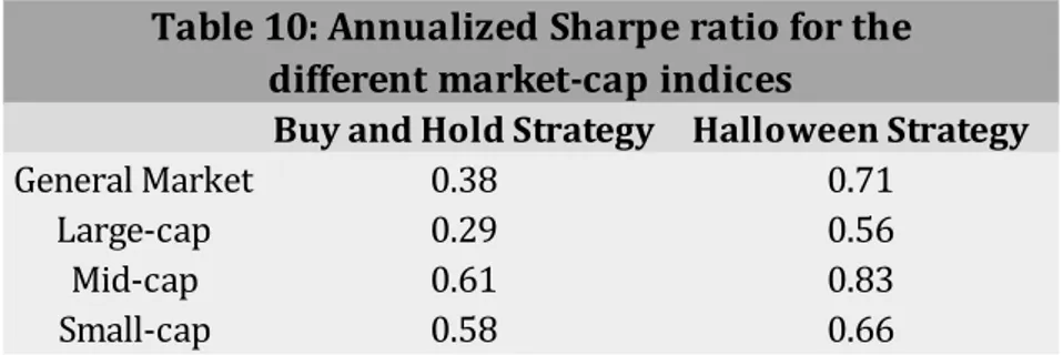
In order to examine the performance of the Halloween strategy and the buy and hold strategy, we have compared the average excess return as well as the standard deviation. In order to define the excess return, a risk-free rate needs to be withdrawn from the monthly return. The risk-free rate that we applied was a Swedish ten-year government bond (Riksbanken, 2020b). Furthermore, the monthly bond rate was then withdrawn from the monthly return in order to get the average excess return. Besides these two measures, we have also used the Sharpe ratio to determine the risk-adjusted performance of the different strategies. Our ambition with this analysis is to provide evidence of whether the Halloween effect can be used as an effective trading strategy that can challenge a buy and hold strategy.
4
Results / Empirical Findings
This section will present the findings from our statistical testing as well as the analysis of the economic significance of the Halloween effect. Furthermore, this section will be divided into three sub-sections that presents the different results from our testing.
4.1
The Halloween Effect in the General Market
In order to test for the Halloween effect in the general Swedish stock market, we investigated the OMXSPI index that includes all listed stocks in Sweden. Our testing framework consisted of hypotheses which exhibited a null hypothesis and an alternative hypothesis. The hypotheses were based on equation 1 and equation 2 that was developed in similarity to Bouman and Jacobsen (2002). In order to test for the statistical significance, we used t-values and determined the significance at a 10, 5 and 1 percent level. If the t-value exceeds the critical value at 10 percent significance, this enable us to reject the null hypothesis. The following equations were constructed to test the statistical significance in the general market:
𝐄𝐪𝐮𝐚𝐭𝐢𝐨𝐧 𝟏: 𝑟𝑖 = 𝜇 + 𝛼1𝐻𝑎𝑙𝑡+ 𝜀𝑡
𝐄𝐪𝐮𝐚𝐭𝐢𝐨𝐧 𝟐: 𝑟𝑖 = 𝜇 + 𝛼1𝐻𝑎𝑙𝑡 𝐴𝑑𝑗
+ 𝛼2𝐽𝑎𝑛𝑡+ 𝜀𝑡
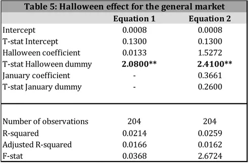
Table 5 displays the results for the Halloween effect in the general market. From equation 1, we can see that there is a positive Halloween coefficient at 1.33 percent. This indicates
Equation 1 Equation 2
Intercept 0.0008 0.0008
T-stat Intercept 0.1300 0.1300
Halloween coefficient 0.0133 1.5272 T-stat Halloween dummy 2.0800** 2.4100**
January coefficient - 0.3661
T-stat January dummy - 0.2600
Number of observations 204 204
R-squared 0.0214 0.0259
Adjusted R-squared 0.0166 0.0162
F-stat 0.0368 2.6724
*p<0.10; **p<0.05; ***p<0.01